Systematic renormalization scheme in light-front dynamics
with Fock space truncation

Abstract

Within the framework of the covariant formulation of light-front dynamics, we develop a general non-perturbative renormalization scheme based on the Fock decomposition of the state vector and its truncation. The counterterms and bare parameters needed to renormalize the theory depend on the Fock sectors. We present a general strategy in order to calculate these quantities, as well as state vectors of physical systems, in a truncated Fock space. The explicit dependence of our formalism on the orientation of the light front plane is essential in order to analyze the structure of the counterterms. We apply our formalism to the two-body (one fermion and one boson) truncation in the Yukawa model and in QED, and to the three-body truncation in a scalar model. In QED, we recover analytically, without any perturbative expansion, the renormalization of the electric charge, according to the requirements of the Ward identity.

I Introduction

The relevance of a coherent relativistic description of few-body systems is now well recognized in particle as well as in nuclear physics. Concerning particle physics, a relativistic formalism is necessary for the understanding of the various components of the nucleon or pion state vectors in terms of valence quarks, gluons, and sea quarks, as revealed, for instance, in exclusive reactions at very high momentum transfer. The need for a coherent relativistic approach to few-body systems has also become clear in nuclear physics in order to check the validity of the standard description of the microscopic structure of nuclei in terms of correlated pion exchanges between nucleons within the general framework of chiral perturbation theory. In this case, electromagnetic interactions play a central role in ”seeing” pion exchanges in nuclei.

In the non-relativistic limit (when the speed of light $c$ goes to infinity) a system of particles is described by its wave function defined at fixed moments of time or, in other words, on the plane $t=\mbox{const}$, and its time evolution is governed by the Schrödinger equation, once the Hamiltonian of the system is known. Relativistic description admits some freedom in choosing the space-like hyper-surface on which the state vector is defined [1]. A possible choice is to take, for this purpose, the same plane $t=\mbox{const}$ (the so-called ”instant” form of dynamics). This is however not very well suited for relativistic systems, since this plane is not invariant under Lorentz boosts. It is much more preferable to use Light-Front Dynamics (LFD) which is of particular interest among various approaches applied so far to study relativistic systems. In the standard version of LFD, the state vector is defined on the plane $t+\frac{\displaystyle{z}}{\displaystyle{c}}=0$ [1], invariant with respect to Lorentz boosts along the $z$ axis.

Advantages of using LFD to describe physical systems are well known. The main one concerns the structure of the vacuum. Because of kinematical constraints, the plus-component $p^{+}\equiv p^{0}+p^{3}$ (we take hereafter $c=1$) of the four-momentum $p$ of any particle state, both real and virtual, is always positive or null. This implies that the vacuum state coincides with the free vacuum, and all intermediate states result from fluctuations of the physical system. One can thus construct any physical system in terms of combinations of free fields, i.e. the state vector is decomposed in a series of Fock sectors with an increasing number of constituents. This enables a systematic calculation of state vectors of physical systems and their observables.

Note that the triviality of the vacuum in LFD, mentioned above, does not prevent from non-perturbative zero-mode contributions (states with $p^{+}=0$, sometimes called the ”vacuum sector”) to field operators, when physical systems with spontaneous symmetry breaking are considered [2]. An application to the $\phi^{4}$ model in $1+1$ dimension has been done in Ref. [3].

While the Fock decomposition is non-perturbative, it is only meaningful if it converges rapidly. One way to look at this convergence for a simple but nevertheless physically relevant system is to investigate, within LFD, the Wick-Cutkosky model: a system of two scalar particles of mass $m$ interacting by the exchange of a massless scalar particle. Independently, the same system can be considered within the four-dimensional Feynman approach by solving the Bethe-Salpeter equation in the ladder approximation which includes exchanges of an infinite number of scalar bosons in the intermediate state. Comparing the results of both calculations [4], we can see that the two- and three-body components of the state vector represent as much as $90\%$ of its norm, for $m=1$ GeV and a coupling constant of $2\pi$ which gives the maximal binding. Such a simple test shows that even in the worst case (a large coupling constant and the exchange of a boson of zero mass) the Fock decomposition is meaningful and may converge rapidly. This however should be analyzed in more realistic calculations.

The decomposition of the state vector of any physical system in terms of Fock sectors on the Light Front (LF) enables a very intuitive interpretation of the physical state, since each Fock sector is reminiscent of a non-relativistic many-body wave function.

The standard version of LFD has however a serious drawback, since the equation of the LF plane $t+z=0$ is not invariant under spatial rotations. As we shall see later on, the breaking of the rotational invariance has many important consequences as far as the construction of bound states with definite angular momentum is concerned, or in the calculation of electromagnetic amplitudes.

To avoid such an unpleasant feature of standard LFD, we shall use below the Covariant formulation of LFD (CLFD) [5, 6], which provides a simple, practical, and very powerful tool in order to describe physical systems as well as their electromagnetic amplitudes. In this formulation, the state vector is defined on the plane characterized by the invariant equation $\omega\makebox[2.27626pt]{$\cdot$}x=0$, where $\omega$ is an arbitrary light-like four-vector with $\omega^{2}=0$. The standard LFD on the plane $t+z=0$ is recovered by considering the particular choice $\omega=(1,0,0,-1)$. The covariance of our approach is caused by the invariance of the LF plane equation $\omega\makebox[2.27626pt]{$\cdot$}x=0$ under any Lorentz transformation of both $\omega$ and $x$. This implies in particular that $\omega$ cannot be kept the same in any reference frame, as it takes place in the standard formulation of LFD with $\omega=(1,0,0,-1)$.

There is of course equivalence, in principle, between the standard and covariant forms of LFD. Within the same approximation (or for exact calculations) CLFD reproduces the results of standard LFD as a particular case. The physical observables should coincide in both approaches, though their derivation in CLFD in most cases is much simpler and more transparent. The relation between CLFD and standard LFD reminds that between the Feynman graph technique and old-fashioned perturbation theory.

CLFD has first been used to investigate the general structure of few-body systems and their electromagnetic observables in the tree approximation (see Ref. [6] for a review). If one wants to go beyond this phenomenological analysis, one has to be able to calculate the state vector of a physical system from a given Hamiltonian in a non-perturbative framework.

Consider, as an example, a system composed of interacting fermion and bosons. In the simple two-body Fock space truncation, the physical fermion state vector is represented as a sum of two sectors: the one single fermion state and the one fermion plus one boson state. The fermion propagator is thus given, in the chain approximation, by the contributions indicated in Fig. 1(a).

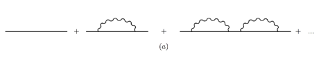
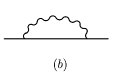
Figure 1: Fermion propagator in the chain approximation, within the two-body Fock space truncation (a) and an irreducible contribution to the perturbative self-energy (b). Solid and wavy lines correspond to fermions and bosons, respectively.

It is non-perturbative in the sense that it involves contributions to all orders in the coupling constant $g$, but approximate, since it incorporates at most two particles in the intermediate states. It is well known that this infinite series can be summed up in terms of the (perturbative) self-energy $\Sigma(p)$ of order $g^{2}$, as indicated in Fig. 1(b). In this two-body truncation, the equivalence between the LF fermion propagator (calculated in CLFD) and the two-point Green’s function (calculated in the Feynman four-dimensional approach) has been shown to occur very naturally to all orders in $g$ [7].

The fermion propagator enters into the expression for the observable fermion-boson scattering amplitude. This amplitude must have a pole, in the $s$-channel, at $s=m^{2}$. To ensure such a property, a Mass Counterterm (MC) must be added to the self-energy. Besides that, the coupling constant coming into the vertices of the diagrams in Fig. 1 can not be identified a priori with the physically observed quantity, but should be treated as some bare (non-renormalized) parameter. In order to calculate physical observables, the boson-fermion Bare Coupling Constant (BCC) as well as the MC should be expressed in terms of the physical coupling constant and the particle masses. This has been done, for the two-body Fock state truncation in CLFD, in Ref. [7]. However, a general renormalization scheme needed to determine the MC and the BCC for the most general case of Fock space truncation has not been proposed yet.

Already at the level of the two-body Fock space truncation, one has to deal with loop diagrams [like the self-energy contribution shown in Fig. 1 (b)]. Their amplitudes diverge for high internal momenta. The implementation of any renormalization scheme essentially depends on the way of regularization of divergent amplitudes. This is indeed a non-trivial task, as it has been already mentioned in various contexts [8, 9]. The regularization of amplitudes in LFD by traditional cutoffs imposed on the transverse and longitudinal components of particle momenta, for instance, corresponds to restricting the integration volume by a rotationally non-invariant domain. The regularized amplitudes depend therefore not only on the size of this domain (i.e., on the cutoff values), but also on its orientation determined by the orientation of the LF plane.

Another source of violation of rotational invariance is the Fock space truncation itself. As a consequence, the number and the structure of the counterterms needed to renormalize the theory depend on the LF plane orientation as well. CLFD allows us to parameterize the latter dependence in a very transparent form, through the four-vector $\omega$. Moreover, the covariant formulation of the approach is mandatory in order to define what are the physical parameters of the theory (and hence to be able to renormalize the latter), since it enables an explicit separation of any spurious contributions depending on $\omega$. This is the case, for instance, for the two-body wave function, as we shall see in Sec. II.

Following the analysis of Ref. [8], we choose the Pauli-Villars (PV) regularization scheme in order to impart mathematical sense to divergent amplitudes. This scheme also preserves rotational invariance, as well as other important symmetries like gauge invariance. Though the PV regularization was developed initially for the four-dimensional Feynman approach, it can be easily implemented into the LFD calculating machinery by simply introducing additional fictitious PV fields [12].

The renormalization procedure must ensure that physical results do not depend on the regularization parameters. Besides that, it should be, first, non-perturbative and, second, consistent with the truncation of the Fock decomposition in the sense that it should not leave any divergences uncancelled.

Let us look, for example, at the renormalization of the fermion propagator in the second order of perturbation theory. There exist three contributions to the physical fermion propagator, as indicated in Fig. 2. These are, from left to right, the free propagator, the self-energy contribution $\Sigma(p)$, and the contribution from the MC $\delta m$. The sum of these three items should be equal, at $p^{2}=m^{2}$, to the free propagator. This fixes $\delta m=-\Sigma(p)$ at ${\not\!p}=m$.

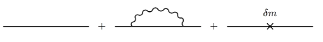
Figure 2: Renormalization of the fermion propagator in the second order of perturbation theory.

As we can see from Fig. 2, Fock sectors with different number of constituents are intimately connected through the renormalization condition: the contribution of the MC (the last diagram in Fig. 2) corresponds to the one-body Fock sector (a single fermion). It should however be opposite, at $\not\!p=m$, to the two-body (one fermion plus one boson) Fock sector contribution given by the second diagram in Fig. 2, in order to cancel its divergence. This means that any MC or, more generally, any bare parameter, should be associated with the number of particles in a given Fock sector. In other words, all MC’s and bare parameters must depend on the Fock sector under consideration. This is a necessary condition.

Several attempts have already been made to address the problem of non-perturbative renormalization in the standard formulation of LFD, either in the Yukawa model (a fermion coupled to scalar bosons) or in QED, using various regularization schemes. Early calculations were performed with a momentum cut-off for the Yukawa model [10] and for QED [11]. As shown in Ref. [8], the use of such a cut-off implies to consider specific counterterms depending on the LF plane orientation. Moreover, the absence of Fock sector dependent counterterms and BCC’s prevents any calculation to converge properly.

The use of PV fields to regulate the amplitudes has first been advocated in Refs. [12] (with three PV bosons) and [13] (with three PV fermions), for the Yukawa model and QED, respectively. These calculations suffer however from the lack of a non-perturbative procedure to determine the parameters of the PV fields, as well as from an incorrect chiral limit. Again, no Fock sector dependent counterterms were considered, which left divergences uncancelled. In particular, this prevents the two-body calculation of QED to reproduce the well known radiative correction to the anomalous magnetic moment of the electron (the Schwinger correction). We shall see in Sec. IV how it arises naturally in our scheme.

Most recent calculations in the Yukawa model with the two- [14] and three-body [15] Fock space truncations used simultaneously a PV fermion and a PV boson to regulate the amplitudes. This regularization procedure is adequate to preserve rotational invariance, at least for the two-body truncation, according to the analysis of Ref. [8]. However these two calculations are plagued with uncancelled divergences.

The dependence of the counterterms on the Fock sectors has been first suggested in Ref. [16] in the context of a simple calculation within the two-body Fock space truncation. This idea has however never been formulated as a coherent renormalization scheme.

The main aim of the present article is to develop such renormalization scheme. We propose a complete and coherent strategy to determine the counterterms and the bare parameters in LFD calculations with a Fock space truncation to any order. A preliminary account of such a scheme was presented in Ref. [17]. We conjecture that this renormalization scheme is also sufficient to avoid any uncancelled divergences in any order of the Fock space truncation, provided appropriate counterterms necessary to recover rotational invariance (if needed) are taken into account. We shall demonstrate below that this is indeed the case for some model and realistic physical systems, within the two- and three-body Fock space truncations.

The plan of our paper is the following. In Sec. II, we recall the main features of the description of bound state systems in CLFD, taking the Yukawa model as an example. We expose in Sec. III our new systematic renormalization scheme in CLFD calculations with Fock space truncation. Applications of this scheme to particular physical systems — to the Yukawa model and QED — within the two-body Fock space truncation (Sec. IV), and to a purely scalar model for the three-body truncation (Sec. V) are then considered. We present our concluding remarks and outline possible perspectives in Sec. VI. Some technical derivations are given in Appendices.

II Description of physical systems in the covariant formulation of light-front dynamics

In order to show how our renormalization scheme should be applied to the analysis of physical systems, we shall consider in the following study the Yukawa model, i.e. a physical fermion composed of a bare fermion coupled to scalar bosons. This system is interesting from several points of view. It is not as simple as a super-renormalizable purely scalar model, while it has many similarities with QED in the Feynman gauge, at least for the case of the simple two-body truncation. It is thus easy to extend our results, as shown in Sec. IV.

II.1 The Yukawa model. Construction of the light-front interaction Hamiltonian

The Lagrangian describing a system of interacting spin-1/2 fermion and scalar boson fields, taking into account the mass renormalization of the fermion, is

$${\cal L}={\cal L}_{F}+{\cal L}_{B}+{\cal L}_{FB},$$ (1)

where the three terms on the r.-h.s. are, respectively, the fermion, boson, and interaction parts,

$${\cal L}_{F} = {\displaystyle i\bar{\Psi}\gamma^{\nu}\partial_{\nu}\Psi-m\bar{\Psi}\Psi,}$$ (2a)

$${\cal L}_{B} = {\displaystyle\frac{1}{2}\left[\partial_{\nu}\Phi\partial^{\nu}\Phi-\mu^{2}\Phi^{2}\right],}$$ (2b)

$${\cal L}_{FB} = {\displaystyle g_{0}\bar{\Psi}\Psi\Phi+\delta m\bar{\Psi}\Psi.}$$ (2c)

Here $\Psi=\Psi(x)$ and $\Phi=\Phi(x)$ are the Heisenberg fermion and boson field operators, $g_{0}$ is the BCC, analogous to the bare charge $e_{0}$ in QED, $m$ is the physical fermion mass, $\mu$ is the physical boson mass, and $\delta m$ is the fermion MC.

As already advocated in Ref. [7], it is more appropriate and physically sounded to construct Fock sectors in terms of free fields corresponding to particles with their physical masses. In that case, one does not have to determine the fermion bare mass $m_{0}$ but rather a MC $\delta m=m_{0}-m$, as it is well known [18]. This choice of the renormalization procedure for the fermion mass is the only way to keep the basis constructed from free fields to be the same in all Fock sectors. In our renormalization scheme the bare parameters like $m_{0}$ depend on the Fock sector in which they appear. If one assigned the bare mass $m_{0}$ to the free fermion field, the latter would be different in different Fock sectors. Taking the free fermion field with the physical mass $m$, on the contrary, fixes it once and for all, while dependence of renormalization parameters on the Fock sectors is carried over to the MC $\delta m$. Moreover, one may hope that the Fock state expansion may converge more rapidly with the use of a fixed physical mass as compared to a (divergent) bare mass.

Working in LFD, we have to deal with Hamiltonians, rather than Lagrangians. Moreover, since we use Fock expansions in terms of free fields, the Hamiltonian must be also expressed through them (i. e. taken in Schrödinger or interaction representation). The general procedure of deriving CLFD Hamiltonians from Lagrangians is exposed in Ref. [7]. First, one should construct the energy-momentum tensor

$$\Theta_{\nu\rho}=\sum_{i}\left(\frac{\partial{\cal L}}{\partial^{\nu}Y_{i}}\right)\partial_{\rho}Y_{i}-g_{\nu\rho}{\cal L},$$ (3)

where $Y_{i}$ denotes either $\Psi$ or $\bar{\Psi}$, or $\Phi$, the sum running over all the fields, and the LF four-momentum operator

$$\hat{P}_{\rho}=\frac{1}{2}\int d\sigma^{\nu}(x)\,\Theta_{\nu\rho},$$ (4)

where the integration is performed on the three-dimensional space element orthogonal to the ”time” direction (the role of time is played in CLFD by the invariant combination $\omega\makebox[2.27626pt]{$\cdot$}x$). The four-momentum operator should then be expressed through the free fields, taking into account constraints imposed on the field components by the equations of motion. The corresponding operator $\hat{P}_{\rho}$ can be represented as the sum

$$\hat{P}_{\rho}=\hat{P}^{(0)}_{\rho}+\hat{P}^{int}_{\rho},$$ (5)

where the two terms on the r.-h.s. are, respectively, the free (i.e. independent of the coupling constant and counterterms) and interaction parts of the four-momentum. The operator $\hat{P}^{int}_{\rho}$ is related to the interaction Hamiltonian $H^{int}(x)$ by

$$\hat{P}^{int}_{\rho}=\omega_{\rho}\int H^{int}(x)\,\delta(\omega\makebox[2.27626pt]{$\cdot$}x)\,d^{4}x.$$ (6)

The calculations performed in Ref. [7] showed that the interaction Hamiltonian for the Yukawa model includes also a set of so-called contact (or instantaneous) terms which explicitly depend on the LF plane orientation and essentially complicate calculations, both perturbative and non-perturbative.

We shall use hereafter the PV regularization which not only maintains rotational invariance, but also kills the contact terms, as will be demonstrated below. The PV scheme can be easily implemented into the Lagrangian [12] by introducing additional fields (we will call them PV fields or PV particles), having negative norm, so that each physical field has its PV counterpart. On the level of free Lagrangians, the physical and PV fields are independent from each other, while they are mixed by the interaction. The PV fermion and PV boson parts of the full Lagrangian are

$${\cal L}_{F,PV} = {\displaystyle-i\bar{\Psi}_{PV}\gamma^{\nu}\partial_{\nu}\Psi_{PV}+m_{1}\bar{\Psi}_{PV}\Psi_{PV},}$$ (7a)

$${\cal L}_{B,PV} = {\displaystyle-\frac{1}{2}\left[\partial_{\nu}\Phi_{PV}\partial^{\nu}\Phi_{PV}-\mu_{1}^{2}\Phi_{PV}^{2}\right],}$$ (7b)

with $m_{1}$ and $\mu_{1}$ being the PV fermion and PV boson masses. Note that the Lagrangians (7) differ by a minus sign from the Lagrangians (2a) and (2b) for the physical fields. The interaction Lagrangian involves all types of fields and has the form

$${\cal L}_{FB,PV}=g_{0}\bar{\Psi}^{\prime}\Psi^{\prime}\Phi^{\prime}+\delta m\bar{\Psi}^{\prime}\Psi^{\prime},$$ (8)

where

$$\Psi^{\prime}=\Psi+\Psi_{PV},\quad\Phi^{\prime}=\Phi+\Phi_{PV}.$$ (9)

The interaction is constructed in such a way that the physical and PV fields come into Eq. (8) on equal grounds. This feature ensures the cancellation of ultra-violet divergencies. The full Lagrangian combining the physical and PV contributions is thus

$${\cal L}_{PV}={\cal L}_{F}+{\cal L}_{B}+{\cal L}_{F,PV}+{\cal L}_{B,PV}+{\cal L}_{FB,PV}.$$ (10)

The Lagrangian (10) generates the interaction Hamiltonian

$$H^{int}_{PV}(x)=-g_{0}\bar{\psi^{\prime}}\psi^{\prime}\varphi^{\prime}-\delta m\bar{\psi^{\prime}}\psi^{\prime}$$ (11)

with $\psi^{\prime}=\psi+\psi_{PV}$ and $\varphi^{\prime}=\varphi+\varphi_{PV}$. The fields $\psi$ and $\psi_{PV}$ ($\varphi$ and $\varphi_{PV}$) satisfy the free Dirac (Klein-Gordon) equations, with the corresponding masses, in contrast to $\Psi$ and $\Phi$ which satisfy the full Heisenberg equation. The main steps leading to Eq. (11) are pointed out in Appendix A.

The Hamiltonian (11) has the traditional spin structure, except for the fact that the ”elementary” fields $\psi^{\prime}$ and $\varphi^{\prime}$ are the sums of the physical and PV fields. In other words, it does not contain any contact terms specific for LFD and explicitly depending on the LF plane orientation. This is a great merit of the PV regularization scheme.

The Lagrangian (8), as well as the Hamiltonian (11), depends on the MC $\delta m$ and on the BCC $g_{0}$. For simplicity, we consider here the case with only one coupling constant to be determined, but our scheme is completely general and can be easily extended to the case where many types of interaction occur.

Apart from the MC and the BCC entering the original Lagrangian, one may also need new counterterms, at the level of the LF Hamiltonian, in order to restore the symmetries broken by the Fock space truncation [10] or by the regularization method [8]. We have already analyzed in Ref. [7] the structure of such counterterms in CLFD, using, as examples, the Yukawa model and QED for the case of the two-body truncation and the standard LF regularization by means of transversal and longitudinal cutoffs. Due to the explicit covariance of CLFD, the general structure of such counterterms can be exhibited in terms of the orientation, $\omega$, of the LF plane. The simplest counterterm which one may consider is given by

$$Z_{\omega}\bar{\psi}\frac{m\not\!\omega}{i\omega\makebox[2.27626pt]{$\cdot$}\partial}\ \psi,$$ (12)

where $Z_{\omega}$ is a constant and $1/i(\omega\makebox[2.27626pt]{$\cdot$}\partial)$ is the operator $1/i\partial^{+}$, Eq. (116), written in covariant notations. This counterterm has a structure similar to that of the MC and appears, in all diagrams, as a factor $Z_{\omega}m{\not\!\omega}/(\omega\makebox[2.27626pt]{$\cdot$}p)$ on each internal fermion line (here $p$ is the four-momentum assigned to the line). Other counterterms with more involved structure may appear if one increases the number of Fock components, giving rise to many-body vertex corrections. The general renormalization scheme we propose in this paper can easily embrace all types of counterterms.

II.2 Covariant formulation of light-front dynamics

In CLFD, the state vector is defined on the LF plane of general orientation $\omega\makebox[2.27626pt]{$\cdot$}x=\xi$, where $\omega$ is an arbitrary four-vector restricted by the condition $\omega^{2}=0$, and $\xi$ is the LF ”time”. We shall take $\xi=0$, for convenience.

Let us recall here, for completeness, how the state vector of a physical system is constructed. In order to avoid congesting notations, we do not consider for the moment PV fields. These fields influence only the explicit form of dynamical operators, but not the general results discussed in this section. PV fields can be easily incorporated later, when we shall study particular physical systems.

We are interested in the state vector, $\phi_{\omega}^{J\sigma}(p)$, of a bound system. It corresponds to definite values for the mass $M$, the four-momentum $p$, and the total angular momentum $J$ with projection $\sigma$ onto the $z$ axis in the rest frame, i.e., the state vector forms a representation of the Poincaré group. This means that it satisfies the following eigenstate equations:

$$\hat{P}_{\rho}\ \phi_{\omega}^{J\sigma}(p) = p_{\rho}\ \phi_{\omega}^{J\sigma}(p),$$ (13a)

$$\hat{P}^{2}\ \phi_{\omega}^{J\sigma}(p) = M^{2}\ \phi_{\omega}^{J\sigma}(p),$$ (13b)

$$\hat{S}^{2}\ \phi_{\omega}^{J\sigma}(p) = -M^{2}\ J(J+1)\ \phi_{\omega}^{J\sigma}(p),$$ (13c)

$$\hat{S}_{3}\ \phi_{\omega}^{J\sigma}(p) = M\ \sigma\phi_{\omega}^{J\sigma}(p),$$ (13d)

where $\hat{S}_{\rho}$ is the Pauli-Lubanski vector

$$\hat{S}_{\rho}=\frac{1}{2}\epsilon_{\rho\nu\alpha\beta}\ \hat{P}^{\nu}\ \hat{J}^{\alpha\beta},$$ (14)

and $\hat{J}$ is the four-dimensional angular momentum operator which is represented, similarly to $\hat{P}_{\rho}$, Eq. (5), as a sum of the free and interaction parts:

$$\hat{J}_{\rho\nu}=\hat{J}^{(0)}_{\rho\nu}+\hat{J}^{int}_{\rho\nu}.$$ (15)

In terms of the interaction Hamiltonian, we have

$$\hat{J}^{int}_{\rho\nu}=\int H^{int}(x)(x_{\rho}\omega_{\nu}-x_{\nu}\omega_{\rho})\delta(\omega\makebox[2.27626pt]{$\cdot$}x)\ d^{4}x.$$ (16)

From the general transformation properties of both the state vector and the LF plane, it follows [19] that

$$\hat{J}^{int}_{\rho\nu}\ \phi_{\omega}^{J\sigma}(p)=\hat{L}_{\rho\nu}(\omega)\phi_{\omega}^{J\sigma}(p),$$ (17)

where

$$\hat{L}_{\rho\nu}(\omega)=i\left(\omega_{\rho}\frac{\partial}{\partial\omega^{\nu}}-\omega_{\nu}\frac{\partial}{\partial\omega^{\rho}}\right).$$ (18)

The equation (17) is called the angular condition. We can now use it in order to replace the operator $\hat{J}^{int}_{\rho\nu}$ entering into Eq. (14) by $\hat{L}_{\rho\nu}(\omega)$. Introducing the notations

$$\hat{M}_{\rho\nu} = \hat{J}^{(0)}_{\rho\nu}+\hat{L}_{\rho\nu}(\omega),$$ (19a)

$$\hat{W}_{\rho} = \frac{1}{2}\epsilon_{\rho\nu\alpha\beta}\ \hat{P}^{\nu}\ \hat{M}^{\alpha\beta},$$ (19b)

we obtain, instead of Eqs. (13c) and (13d):

$$\hat{W}^{2}\phi_{\omega}^{J\sigma}(p) = -M^{2}J(J+1)\ \phi_{\omega}^{J\sigma}(p),$$ (20a)

$$\hat{W}_{3}\ \phi_{\omega}^{J\sigma}(p) = M\ \sigma\ \phi_{\omega}^{J\sigma}(p).$$ (20b)

These equations do not contain the interaction Hamiltonian, once $\phi$ satisfies Eqs. (13a) and (13b). The construction of the wave functions of states with definite total angular momentum becomes therefore a purely kinematical problem. Indeed, the transformation properties of the state vector under rotations of the coordinate system is fully determined by its total angular momentum, while the dynamical part of the latter is separated out by means of the angular condition. The dynamical dependence of the wave functions on the LF plane orientation now turns into their explicit dependence on the four-vector $\omega$ [6]. Such a separation, in a covariant way, of kinematical and dynamical transformations is a definite advantage of CLFD as compared to standard LFD on the plane $t+z=0$.

II.3 General Fock decomposition of the state vector

According to the general properties of LFD, mentioned in the Introduction, we decompose the state vector of a physical system in Fock sectors. Schematically, we have

$$\phi^{J\sigma}_{\omega}(p)\equiv|1\rangle+|2\rangle+\dots+|n\rangle+\dots$$ (21)

Each term on the r.-h.s. denotes a state with a fixed number of particles from which the physical system can be constructed. In the Yukawa model the analytical form of the Fock decomposition is

$$\phi^{J\sigma}_{\omega}(p) = \sum_{n=1}^{\infty}\frac{(2\pi)^{3/2}}{(n-1)!}\sum_{\sigma^{\prime}}\int\phi_{n,\sigma\sigma^{\prime}}(k_{1}\ldots k_{n},p,\omega\tau_{n})a^{{\dagger}}_{\sigma^{\prime}}({\bf k}_{1})c^{{\dagger}}({\bf k}_{2})\ldots c^{{\dagger}}({\bf k}_{n})|0\rangle$$ (22)

$$\times \delta^{(4)}(k_{1}+\ldots+k_{n}-p-\omega\tau_{n})2(\omega\makebox[2.27626pt]{$\cdot$}p)d\tau_{n}\prod_{l=1}^{n}\frac{d^{3}k_{l}}{(2\pi)^{3/2}\sqrt{2\varepsilon_{k_{l}}}},$$

where $\phi_{n,\sigma\sigma^{\prime}}(\ldots)$ is the $n$-body LF wave function (Fock component) describing the state made of one free fermion and $(n-1)$ free bosons, $a^{{\dagger}}$ ($c^{\dagger}$) are the free fermion (boson) creation operators, $\varepsilon_{k_{l}}=\sqrt{{\bf k}_{l}^{2}+m_{l}^{2}}$, and $m_{l}$ is the mass of the particle $l$ with the four-momentum $k_{l}$. The combinatorial factor $1/(n-1)!$ is introduced in order to take into account the identity of bosons. The variables $\tau_{n}$ describe how far off the energy shell the constituents are. As explained in Appendix B, the momentum $\omega\tau_{n}$ can be identified with a fictitious particle, called spurion. In practical calculations, the infinite sum over $n$ is truncated by retaining terms with $n$ which does not exceed a given number $N$, while those with $n>N$ are neglected. Decompositions analogous to Eq. (22) can be easily written for the QED case [7] or for a purely scalar system [20].

The normalization condition for the state vector is given by

$$\phi^{{\dagger}\,J\sigma^{\prime}}_{\omega}(p^{\prime})\phi^{J\sigma}_{\omega}(p)=2\varepsilon_{p}\ \delta_{\sigma,\sigma^{\prime}}\delta^{(3)}(\bf{p}-\bf{p^{\prime}}).$$ (23)

Being rewritten through the CLFD wave functions, it has the form

$$\sum_{n=1}^{\infty}I_{n}=1,$$ (24)

where

$$I_{n} = \frac{(\omega\makebox[2.27626pt]{$\cdot$}p)}{(2\pi)^{3(n-1)}(n-1)!}$$

$$\times\int\left(\prod_{l=1}^{n}\frac{d^{3}k_{l}}{2\varepsilon_{k_{l}}}\right)d\tau_{n}\delta^{(4)}\left(\sum_{l=1}^{n}k_{l}-p-\omega\tau_{n}\right)$$

$$\times\sum_{\sigma,\sigma^{\prime}}\phi_{n,\sigma\sigma^{\prime}}^{{\dagger}}\phi_{n,\sigma\sigma^{\prime}}^{\vphantom{{\dagger}}}$$ (25)

is the relative contribution of the $n$-body sector to the full norm. For shortness, we omitted the arguments of the wave functions. The factor $1/(n-1)!$ in Eq. (25) appears as a combined effect caused by the presence of the same factor in Eq. (22) and by the contraction of the creation and annihilation operators, when calculating the l.-h.s. of Eq. (23).

As follows from the discussion in Sec. II.2, the spin structure of the wave functions $\phi_{n,\sigma\sigma^{\prime}}$ is very simple, since it is purely kinematical, but it should incorporate $\omega$-dependent components in order to fulfill the angular condition (17). It is convenient to decompose each wave function $\phi_{n,\sigma\sigma^{\prime}}$ into invariant amplitudes constructed from the particle four-momenta (including the four-vector $\omega$!) and spin structures (matrices, bispinors, etc.). In the Yukawa model, for instance, we have

$$\phi_{1,\sigma\sigma^{\prime}} = \psi_{1}\ \bar{u}_{\sigma^{\prime}}(k_{1})u_{\sigma}(p),$$ (26a)

$$\phi_{2,\sigma\sigma^{\prime}} = \bar{u}_{\sigma^{\prime}}(k_{1})\left[\psi_{2}+\psi^{\prime}_{2}\ \frac{m\not\!\omega}{\omega\makebox[2.27626pt]{$\cdot$}p}\right]u_{\sigma}(p),$$ (26b)

since no other independent spin structures can be constructed. Here $u$’s are bispinors, $\psi_{1}$, $\psi_{2}$, and $\psi_{2}^{\prime}$ are scalar functions determined by the dynamics. For a spin $1/2$ system coupled to scalar particles, the number of invariant amplitudes for the two-body Fock component coincides with the number of independent amplitudes of the reaction $\mbox{spin}\ 1/2+\mbox{scalar}\to\mbox{spin}\ 1/2+\mbox{scalar}$, which is $(2\times 2)/2=2$, due to parity conservation.

Note that the formulas (22), (25), and (26) are written for the state vector which contains physical particles only. The use of the PV regularization, strictly speaking, changes them. However, their generalization is straightforward. We do not give here the corresponding general relations, but give their particular forms when we proceed to the consideration of concrete physical systems.

II.4 Eigenstate equation

The equations for the Fock components can be obtained from Eq. (13b) by substituting there the Fock decomposition (22) of the state vector $\phi(p)$ (here and below we will omit, for shortness, all indices in the notation of the state vector) and calculating the matrix elements of the operator $\hat{P}^{2}$ in Fock space. With the expressions (5) and (6), we can easily get the eigenstate equation [20]:

$$2(\omega\makebox[2.27626pt]{$\cdot$}p)\int\tilde{H}^{int}(\omega\tau)\frac{d\tau}{2\pi}\phi(p)=-\left[\left(\hat{P}^{(0)}\right)^{2}-M^{2}\right]\phi(p),$$ (27)

where $\tilde{H}^{int}$ is the interaction Hamiltonian in momentum space:

$$\tilde{H}^{int}(\omega\tau)=\int H^{int}(x)e^{-i(\omega\makebox[2.27626pt]{$\cdot$}x)\tau}d^{4}x.$$ (28)

For the Yukawa model with the PV regularization, $H^{int}(x)$ is given by Eq. (11).

According to the decomposition (22), the conservation law for the momenta in each Fock component has the form

$$k_{1}+k_{2}+\cdots+k_{n}=p+\omega\tau_{n}.$$ (29)

Hence, the action of the operator $\left(\hat{P}^{(0)}\right)^{2}-M^{2}$ on the state vector reduces to the multiplication of each Fock component by the factor $(\sum_{l=1}^{n}k_{l})^{2}-M^{2}=2(\omega\makebox[2.27626pt]{$\cdot$}p)\tau_{n}$. It is therefore convenient to introduce the notation

$${\cal G}(p)=2(\omega\makebox[2.27626pt]{$\cdot$}p)\hat{\tau}\phi(p),$$ (30)

where $\hat{\tau}$ is the operator which, acting on a given component $\phi_{n,\sigma\sigma^{\prime}}$ of $\phi(p)$, gives $\tau_{n}\phi_{n,\sigma\sigma^{\prime}}$. ${\cal G}(p)$ has the Fock decomposition which is obtained from Eq. (22) by the replacement of the wave functions $\phi_{n,\sigma\sigma^{\prime}}$ by the vertex functions $\Gamma_{n}$ (which we will also refer to as the Fock components) defined by

$$\bar{u}_{\sigma^{\prime}}(k_{1})\Gamma_{n}u_{\sigma}(p)=(s_{n}-M^{2})\phi_{n,\sigma\sigma^{\prime}}$$ (31)

and $s_{n}=(k_{1}+\ldots k_{n})^{2}$. Since for each Fock component $s_{n}-M^{2}=2(\omega\makebox[2.27626pt]{$\cdot$}p)\tau_{n}$, we can cast the eigenstate equation in the form

$${\cal G}(p)=\frac{1}{2\pi}\int\left[-\tilde{H}^{int}(\omega\tau)\right]\frac{d\tau}{\tau}{\cal G}(p)\ .$$ (32)

The physical bound state mass $M$ is found from the condition that the eigenvalue is 1. This equation is quite general and equivalent to the eigenstate equation (13b). It is non-perturbative.

The normalization integrals (25) rewritten through the vertex functions are

$$I_{n} = \frac{(\omega\makebox[2.27626pt]{$\cdot$}p)}{(2\pi)^{3(n-1)}(n-1)!}$$ (33)

$$\times\int\left(\prod_{l=1}^{n}\frac{d^{3}k_{l}}{2\varepsilon_{k_{l}}}\right)d\tau_{n}\delta^{(4)}\left(\sum_{l=1}^{n}k_{l}-p-\omega\tau_{n}\right)$$

$$\times\frac{\mbox{Tr}\{({\not\!p}+M)\bar{\Gamma}_{n}({\not\!k}_{1}+m)\Gamma_{n}\}}{(s_{n}-M^{2})^{2}}$$

with $\bar{\Gamma}_{n}=\gamma^{0}\Gamma_{n}^{{\dagger}}\gamma^{0}$.

Since the Hamiltonian (11) has the ordinary structure in terms of the fields $\psi^{\prime}$ and $\varphi^{\prime}$ (i.e. it does not include any contact terms), we may apply, for subsequent calculations, the standard CLFD graph technique rules [6] with minor changes (see Appendix B).

III Systematic Renormalization Scheme in CLFD

In the usual renormalization scheme, the bare parameters are determined by fixing some physical quantities like the particle masses and the physical coupling constant. The physical parameters are thus expressed through the bare ones. This identification implies in fact the following two important consequences which are usually never clarified in LFD calculations, but are at the heart of our scheme.

(i) In order to express the physical parameters through the bare ones, and vice versa, one should be able to calculate observables or, in other words, physical amplitudes. In LFD, any physical amplitude is represented as a sum of partial contributions, each depending on the LF plane orientation. Since an observable quantity can not depend on the choice of the LF plane, this spurious dependence must cancel in the whole sum. Such a situation indeed takes place, for instance, in perturbation theory, provided the regularization of divergencies in LFD amplitudes is done in a rotationally invariant way [8]. In non-perturbative LFD calculations which are always approximate (say, due to the Fock space truncation we just use here) the dependence on the LF plane orientation may survive even in physical amplitudes. For this reason, the identification of such amplitudes with observable quantities becomes ambiguous and expressing the amplitudes through the physical parameters turns into a non-trivial problem.

When working in standard LFD on the plane $t+z=0$, one may think that even approximate LFD amplitudes do not depend on the LF plane orientation. As a matter of fact, they do, but this dependence is simply hidden. It reflects itself by the non-invariance of the corresponding amplitudes: the result of calculation is affected by the choice of the reference frame.

As we have detailed in Sec. II, CLFD is a unique tool to control this dependence in terms of the arbitrary light-like four-vector $\omega$ specifying the LF plane orientation. We shall see in Sec. IV how one should make use of this property to define the physical fermion-boson coupling constant from the two-body Fock component of the type (26b).

(ii) The explicit form of the relationship between the bare and physical parameters depends on the approximation which is made. This is trivial in perturbation theory where the order of approximation is distinctly determined by the power of the coupling constant. In our non-perturbative approach based on the truncated Fock decomposition an analogous parameter is absent. At the same time, to make calculations compatible with the order of truncation, one has to trace somehow the level of approximation. This implies that, on general grounds, the bare parameters should depend on the Fock sector in which they are considered. Moreover, this dependence must be such that all divergent contributions are cancelled.

We will show in the following how to realize the renormalization procedure in practice. For clarity, we take, as a background, a model of interacting fermions and bosons like the Yukawa model or QED. At the same time, let us emphasize once more that the general renormalization strategy developed here is applicable to physical systems with arbitrary interaction admitting Fock decomposition of the state vector.

III.1 Fock sector dependent counterterms

Let us call $N$ the maximal number of Fock sectors considered in a given approximation, and $n$ the number of constituents in a given Fock sector [one fermion and $(n-1)$ bosons]. We have $n\leq N$. Each Fock sector is described by its vertex function defined by Eq. (31). In a truncated Fock decomposition, each vertex function should depend on $N$. We shall thus denote it by $\Gamma_{n}^{(N)}$. Graphically, $\Gamma_{n}^{(N)}$ can be represented by the diagram shown in Fig. 3.

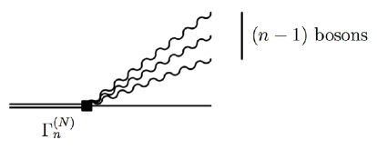
Figure 3: Vertex function of order $n$ for the $N$-body Fock space truncation.

III.1.1 Mass counterterm

The simple example of the fermion self-energy renormalization by the MC within the two-body Fock space truncation, presented in the Introduction, can serve as a guideline to define our general rules. In this example, the MC should be labelled with a subscript and denoted by $\delta m_{2}$, in order to indicate that it is introduced in order to cancel, at $p\!\!\!/=m$, the fermion self-energy contribution which belongs to the two-body Fock sector. In other words, $\delta m_{2}$ is related, by construction, to the two-body state, even though it is attached to a single fermion line. More generally, the subscript at $\delta m$ corresponds to the maximal number of particles in which the fermion line where the MC is attached can fluctuate, so that the total number of particles at any LF time equals $N$. In the given example it is $2$.

Let thus denote by $\delta m_{l}$ the MC in the most general case. Since we truncate our Fock space to order $N$, one should make sure that, at any LF time, the total number of particles is at most $N$. Our first rule is thus:

• in any amplitude where the MC $\delta m_{l}$ appears, the value of $l$ is such that the total number of bosons in flight plus $l$ equals the maximal number of Fock sectors considered in the calculation, i.e. $N$.

For instance, in the typical contribution indicated in Fig. 4, the MC is $\delta m_{(N-n+1)}$. Indeed, since there are already $(n-1)$ bosons in flight, the fermion line can fluctuate in at most $l=(N-n+1)$ particles, so that the total number of particles at a given LF time is just $(N-n+1)+(n-1)=N$ and no more.

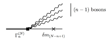
Figure 4: Typical MC insertion.

In order to calculate the whole set of the MC’s $\delta m_{l}$ one should proceed in the following way. Any calculation of the state vector within the Fock space truncation of order $N$ involves the MC’s $\delta m_{l}$ with $l=1,2,\dots N$. We emphasize at this point that the MC’s $\delta m_{l}$ are successive approximations to the true MC $\delta m$ appearing in the original Hamiltonian. They are connected to each other by some kind of recursion in the sense that finding $\delta m_{l}$ requires knowledge of the lower order counterterms, i.e. $\delta m_{1}$, $\delta m_{2}$, .. $\delta m_{l-1}$. This is analoguous to what happens in any perturbative calculation where each MC relates to a definite order of perturbation theory.

For the MC of lowest order, we simply have

$$\delta m_{1}=0,$$ (34)

which is trivial since if the fermion can not fluctuate in more than one particle, its mass is not renormalized at all. The subsequent MC’s are calculated by solving successively the eigenvalue equations for the Fock components for the $2,3,\dots N$-body Fock space truncations.

III.1.2 Bare coupling constant

Let us now come to the determination of the BCC. The general strategy we developed above for the calculation of the MC should of course be also applied to the BCC case, with however a bit of caution, since the BCC may enter in two different types of contributions.

• The first one appears in the calculation of the state vector itself, when Eq. (32) is solved. In that case, any boson-fermion coupling constant is associated with the emission or the absorption of a boson which participates in the particle counting, in accordance with the rules detailed above, since it is a part of the state vector.

• The second one appears in the calculation of the boson-fermion scattering amplitude or of the boson-fermion three-point Green’s function (3PGF) like the electromagnetic form factor in the case of QED. This observable is usually considered, at some kinematical point, to define the physical coupling constant. Now the external boson is an (asymptotic) free field rather than a part of the state vector. The particle counting rule advocated above should therefore not include the external boson line.

One has thus to distinguish two types of BCC’s: $g_{0}$ and $\bar{g}_{0}$ describing, respectively, the interaction vertices of the fermion with internal and external bosons. As we shall see below, these two BCC’s are found from different conditions and do not coincide with each other for a finite order Fock space truncation.

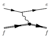
Figure 5: Typical contribution to the two-body scattering amplitude of a probe on a bound state system.

The necessity to introduce two BCC’s can be also explained from another point of view. Let us consider the scattering amplitude of a given probe on a bound state system. Such scattering amplitude can be represented by the diagram in Fig. (5). The in and out asymptotic states are defined in terms of the (structureless) probe denoted by $e$ and the bound state system denoted by $f$. The state vector of the bound system is calculated within a given approximation (the Fock space truncation, in our case), starting from a known Hamiltonian. Therefore, the calculated state vector ”knows” nothing about the subsequent interaction it can have with the probe, i.e. it should be independent of any coupling to the external virtual bosons exchanged between the probe and the bound system.

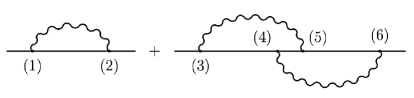
Figure 6: Two- and three-body Fock sector contributions to the fermion self-energy.

Similarly to the MC, the BCC’s should also keep track of the Fock sector in which they appear. To illustrate this fact, let us write down some typical contributions to the fermion self-energy, involving at most two bosons in flight (i.e. for $N=3$). They are shown in Fig. 6. All the vertices are described by the internal BCC’s, since the self-energy is a part of the fermion state vector. The vertices $(1)$ and $(2)$ involve the BCC’s attached to the two-body sector in three-body truncated Fock space. So, each of these vertices or both can be ”dressed” by one more bosonic loop, as indicated for the vertices $(4)$ and $(5)$. The latter vertices correspond to states fully ”saturated” with bosons. In other words, no radiative corrections to them are allowed in the given approximation. From here it follows that the vertices $(1)$–$(3)$ and $(6)$, on the one hand, and $(4)$ and $(5)$, on the other hand, are described by different BCC’s. Analogously to the MC, we will denote each internal BCC by $g_{0l}$, where the subscript $l$ indicates which Fock sector the given BCC belongs to. We can then formulate the general rule:

• in any amplitude which couples constituents inside the state vector one should attach to each vertex the internal BCC $g_{0l}$. The value of $l$ is such that the total number of bosons in flight before (after) the vertex - if the latter corresponds to the boson emission (absorbtion) - plus $l$ equals the maximal number of the Fock sectors considered in the calculation, i.e. $N$.

Applying this rule to the diagrams shown in Fig. 6, we find that the vertices $(1)$–$(3)$ and $(6)$ are described by the BCC $g_{03}$ [no bosons in flight before the vertices $(1)$ and $(3)$ or after the vertices $(2)$ and $(6)$], while the vertices $(4)$ and $(5)$ are described by the BCC $g_{02}$ (one boson in flight before or after each vertex). The BCC $g_{02}$ is calculated within the two-body Fock space truncation and enters into the calculations within the three-body truncation as a known parameter, while $g_{03}$ should be found. When considering the four-body truncation, one should then calculate $g_{04}$, knowing both BCC’s $g_{02}$ and $g_{03}$. The procedure can thus be extended to arbitrary $N$.

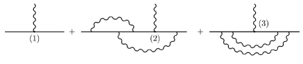
Figure 7: Typical contribution to the fermion-boson 3PGF.

Let us finally consider typical contributions to the 3PGF, analogous to those for the self-energy, as discussed above. Some of them are presented in Fig. 7. The crucial difference with the self-energy case consists in that the bosons emitted from the vertices $(1)$–$(3)$ are absorbed by an external particle (typically an external probe) which is not included into the state vector. For this reason, the vertices $(1)$–$(3)$ are described by the external BCC’s $\bar{g}_{0l}$, while all the others correspond to the internal BCC’s $g_{0l}$. The values of $l$ for the ”internal” vertices are determined according to the rule specified above, with the only exception that the external boson does not take part in the particle counting. For the ”external” vertices $(1)$–$(3)$ the situation is quite similar. The vertices $(1)$ and $(2)$ corresponding to the two-body Fock sector (the external boson is not counted!) admit additional corrections, within the three-body Fock space truncation, from ”internal” bosonic loops, while the vertex $(3)$ does not, since it appears within the three-body sector. We can conclude from here that the external BCC’s attached to the vertices $(1)$ and $(2)$ should differ from that for the vertex $(3)$. We can thus formulate the following general rule:

• in any amplitude which couples constituents of the state vector with an external field, one should attach to the vertex involving this external field the external BCC $\bar{g}_{0l}$. The value of $l$ is such that, at the LF time corresponding to the vertex, the total number of internal bosons in flight - i.e. those emitted and absorbed by particles entering the state vector - plus $l$ equals the maximal number of the Fock sectors considered in the calculation, i.e. $N$.

This rule prescribes to attach to the vertices $(1)$ and $(2)$ in Fig. 7 the BCC $\bar{g}_{02}$, while the vertex $(3)$ is associated with $\bar{g}_{01}$.

The lowest order BCC’s are

$$g_{01} = 0,$$ (35a)

$$\bar{g}_{01} = g.$$ (35b)

Eq. (35a) is trivial, because no fermion-boson interaction is allowed in the one-body Fock space truncation. Eq. (35b) reflects the fact that the external BCC, in the same approximation, is not renormalized at all since a single fermion can not be ”dressed”.

Note that the rule for attaching BCC’s to external vertices holds unchanged if the external field is a particle of another sort than the bosons entering into the state vector. Such a situation takes place, for instance, when one calculates the electromagnetic vertex of a fermion, when the state vector does not contain photons (e.g. in the Yukawa model). Evidently no problems with particle counting arise in this case.

Some illustrations of the rules concerning the internal and external BCC’s are given in Fig. 8.

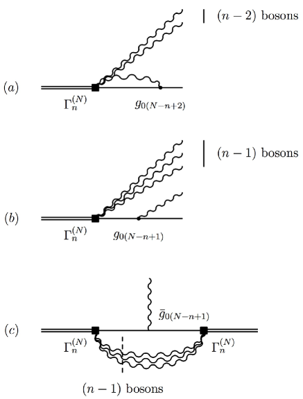
Figure 8: Typical contributions to the fermion state vector for the absorption (a) and the emission (b) of an internal boson, and to the fermion-boson 3PGF (c).

This completes the set of our general rules to define in a systematic and non-perturbative way the MC and the BCC’s in LFD calculations within truncated Fock space. The three rules exposed above have very similar logical grounds based on the particle counting in intermediate states. Namely, the index $l$ at the MC and the BCC’s is always calculated by the same rule: $l$ equals the difference between the order of approximation $N$ and the number of internal bosons in flight at the corresponding LF time.

Though we rely on the fermion-boson model when weconsidered the above procedure, this latter can be easily extended to other systems with additional counterterms and bare parameters.

III.2 Renormalization Conditions

Once proper bare parameters and counterterms have been identified, one should fix them from a set of renormalization conditions. In perturbation theory, there are three quantities to be determined: the fermionic MC, the BCC, and the norm of the fermion field (if the boson field renormalization is not considered). Usually, the on-mass-shell renormalization is applied, with the following conditions. The MC is fixed from the requirement that the two-point Green’s function has a pole at $p^{2}=M^{2}$, where $M$ is the physical mass of the fermion. The fermion field normalization is fixed by the condition that the residue of the two-point Green’s function in the pole is $1$. The BCC is determined by requiring that the on-mass-shell 3PGF is given by the product of the physical coupling constant and the elementary (i.e. not ”dressed”) vertex.

One should now extend these conditions in order to determine the bare parameters and the counterterms in a non-perturbative LFD framework. We do not need to renormalize the fields in our approach, since we deal with already normalized state vectors. It remains to specify the procedure to find the set of MC’s $\delta m_{l}$ and the BCC’s $\bar{g}_{0l}$ and $g_{0l}$.

The eigenstate equation for the state vector in the $N$-body approximation includes two unknown parameters, the MC $\delta m_{N}$ and the BCC $g_{0N}$, while all $\delta m_{l}$ and $g_{0l}$ with $l\leq N-1$ are defined from calculations made for Fock space truncations of lower orders. Provided $g_{0N}$ is fixed, the MC $\delta m_{N}$ is found from the condition that the eigenvalue in Eq. (32) equals 1 in the limit where the mass of the ground state, $M$, is equal to the mass of the fermionic constituent, $m$. To determine $g_{0N}$, one should relate it to the physical coupling constant. For instance, in the traditional QED renormalization scheme, the BCC is found from the requirement that the residue of the photon-electron scattering amplitude in the pole $s=m^{2}$, where $s$ is the invariant energy squared of the system electron + photon, would be proportional to the physical electron charge squared. This condition is not restricted to perturbation theory and can be directly extended to non-perturbative approaches as well. In our language, it is equivalent to require that the two-body vertex $\Gamma_{2}$ is proportional, at $s=m^{2}$, to the elementary vertex, the proportionality coefficient being just the physical coupling constant. For example, one has to require, at $s=m^{2}$, that $\Gamma_{2}=g$ in the Yukawa model, and $\Gamma_{2}^{\nu}=e\gamma^{\nu}$ in QED. From here a relation between the internal BCC and the physical coupling constant can be derived.

To determine the external BCC, a similar condition should be imposed on the 3PGF. Indeed, the two-body vertex and the 3PGF represent two different channels of the same reaction. Hence, taken entirely on the mass and energy shells, they must coincide. It follows from here that the 3PGF $G(p,p^{\prime})$, where $p$ ($p^{\prime}$) is the four-momentum of the incoming (outgoing) fermion, reduces, at $p^{2}={p^{\prime}}^{2}=m^{2}$ and $q^{2}\equiv(p^{\prime}-p)^{2}=\mu^{2}$, to the same product of the elementary vertex and the physical coupling constant. Since the internal BCC has already been found from the calculation of $\Gamma_{2}$, the above condition on the 3PGF allows to relate the external BCC with the physical coupling constant.

Note that the analytical continuation of the two-body vertex function and the 3PGF to the non-physical points $s=m^{2}$ and $q^{2}=\mu^{2}$ does not encounter any technical difficulties, even in numerical calculations, since we can use for this aim the eigenstate equation (32). Its l.-h.s. contains the function to be continued in the non-physical point. From the r.-h.s., both $\Gamma_{2}$ and 3PGF are expressed through integrals involving the vertex functions in the physical domain, whereas the dependence of the integrand on $s$ and $q^{2}$ is explicit. We can put there $s=m^{2}$ and $q^{2}=\mu^{2}$.

In perturbation theory, the equivalence of the on-mass-shell two-body vertex function and 3PGF (calculated in the same order!) appears automatically, as a consequence of the analytical properties of scattering amplitudes. For this reason, it does not make any sense to distinguish the external and internal BCC’s, because they are equal to each other to any order. The same would happen in exact calculations, if they were possible. In our non-perturbative approach based on truncated Fock decompositions, the non-renormalized two-body vertex function and the 3PGF, even taken on the energy shell, do not automatically coincide , in any finite order approximation. Moreover, they may be not constant (i.e. keep dependence on particle momenta) and depend also on the LF plane orientation (on the four-vector $\omega$, in CLFD). If so, the question how to identify such objects with physical constants in the renormalization point requires special consideration.

First of all, one has to fix unambiguously all kinematical variables in the renormalization point, in order that both the two-body vertex function and the 3PGF would turn into constants. Concerning the 3PGF, we can offer a universal solution of this problem. Indeed, $G(p,p^{\prime})$ depends dynamically on two scalar variables, say, $q^{2}$ and $\omega\makebox[2.27626pt]{$\cdot$}q/\omega\makebox[2.27626pt]{$\cdot$}p$. The condition $q^{2}=\mu^{2}$ fixes the first variable, but leaves free the second one. However, if one imposes the condition $\omega\makebox[2.27626pt]{$\cdot$}q=0$ (analogous to $q^{+}=0$ in ordinary LFD) on the four-vector $\omega$, the dependence of the 3PGF on the second variable drops out, and it becomes a constant at fixed $q^{2}$. This condition is also necessary for the factorization of the total scattering amplitude of a probe on the physical system under study, in terms of the external boson propagator and the 3PGF. In practice, one should calculate $G(p,p^{\prime})$, keeping $\omega\makebox[2.27626pt]{$\cdot$}p=\omega\makebox[2.27626pt]{$\cdot$}p^{\prime}$, and then continue it analytically, as a function of only one variable $q^{2}$ to the point $q^{2}=\mu^{2}$.

The two-body vertex $\Gamma_{2}$ also depends dynamically on two scalar variables, e.g. $s$ and $x\equiv\omega\makebox[2.27626pt]{$\cdot$}k_{2}/\omega\makebox[2.27626pt]{$\cdot$}p$, where $k_{2}$ is the boson four-momentum. The condition $s=m^{2}$ does not fix $x$. In an exact calculation, $\Gamma_{2}$ at $s=m^{2}$ does not depend on $x$, while the $x$-dependence survives because of approximations. Therefore, some additional restriction must be imposed on $x$. Unfortunately, a universal choice how to fix $x$ is hardly possible, in contrast to the case of the 3PGF. This problem should be solved separately, for each particular physical system.

Once the kinematics in the renormalization point is fixed, both the two-body vertex function and the 3PGF turn, in this point, into constant matrices. Their dependence on the LF plane orientation may however survive. For example, in the Yukawa model, the term $\psi^{\prime}_{2}\ {m\not\!\omega}/{(\omega\makebox[2.27626pt]{$\cdot$}p)}$ in the two-body wave function (26b), which explicitly depends on $\omega$, implies analogous dependence in the two-body vertex function, unless $\psi^{\prime}_{2}=0$ in the renormalization point. To get rid of it, one should insert new counterterms into the LF Hamiltonian, also explicitly depending on $\omega$, which cancel completely the $\omega$-dependent term in $\Gamma_{2}$. Additional counterterms may also be needed to kill possible $\omega$-dependence of the 3PGF. According to the general renormalization strategy, these counterterms must depend on the Fock sector under consideration, in full analogy with the MC and the BCC’s.

Introducing the internal and external BCC’s and imposing the above renormalization conditions on both the on-energy-shell two-body vertex and 3PGF, we force their coincidence, after renormalization, for arbitrary Fock space truncation of finite order. At this level, we restore the cross-invariance of scattering amplitudes in the renormalization point.

Summarizing, we propose the following non-perturbative renormalization conditions:

• The MC is fixed by solving the eigenstate equation (32) in the limit $M\to m$, where $M$ is the mass of the ground state of the physical system, and $m$ is the physical mass of the fermionic constituent.

• The state vector is normalized according to the standard condition (23).

• The internal bare coupling constant $g_{0l}$ is fixed from the condition that the $\omega$-independent part of the two-body vertex function taken at $s=m^{2}$ and at a given value of $x$, denoted by $x^{*}$, is proportional to the elementary vertex, with the proportionality coefficient being the physical coupling constant.

• The external bare coupling constant $\bar{g}_{0l}$ is fixed from the condition that the $\omega$-independent part of the 3PGF calculated at $\omega\makebox[2.27626pt]{$\cdot$}q=0$ and taken at $q^{2}=\mu^{2}$ is proportional to the elementary vertex, with the proportionality coefficient being the physical coupling constant.

• The $\omega$-dependent counterterms in the Hamiltonian are fixed by the conditions that the $\omega$-dependent parts of the two-body vertex function in the point ($s=m^{2},x^{*})$ and the 3PGF in the point $(q^{2}=\mu^{2},\omega\makebox[2.27626pt]{$\cdot$}q=0)$ are zero.

• The values of all bare parameters and counterterms for $l\leq N$ are determined from successive calculations within the $1,2,\dots N$ Fock space truncations.

IV Applications to the N=2 Fock space truncation

In order to show simple but nevertheless meaningful applications of the general renormalization scheme developed above, we consider, in a first step, the Yukawa model. The LF Hamiltonian including PV fields has been derived in Sec. II. We shall then extend our results to QED which is very similar to the Yukawa model for the $N=2$ Fock space truncation. To simplify notations, we will omit in the following the superscript $(N)$ at each vertex function.

IV.1 Yukawa model

IV.1.1 Solution of the eigenstate equation

The solution of the eigenstate equation (32) within the $N=2$ Fock space truncation has already been found in Ref. [7]. Sharp cut-offs imposed on the longitudinal and transverse components of particle momenta were used to regularize the amplitudes. We revisit here the same problem, but apply the PV regularization method (with one PV fermion and one PV boson), as advocated in Sec. II. Besides that, we shall apply and test the new renormalization scheme proposed in Sec. III.

The use of the PV regularization extends Fock space: instead of one Fock component for the one-body sector we have now two components corresponding to the physical and PV fermions, while the two-body sector is described by four components related to the states either with both physical particles, or with the physical fermion plus the PV boson, or with the PV fermion plus the physical boson, or, finally, with both PV particles. The extension of Fock space makes the computational analysis more cumbersome, but this is compensated by the simplification of the equations for the Fock components due to the disappearance of the contact terms, as well as the absence of spurious $\omega$-dependent contributions to the fermion self-energy [8].

To incorporate the PV particles into the state vector, we will supply the vertex functions, as well as the particle momenta and masses, with the indices $i$ and $j$ which relate, respectively, to fermions and bosons. Each index is either $0$ for a physical particle or $1$ for a PV one. All particle momenta are on their mass shells:

$$k_{i}^{2}=m_{i}^{2},\quad k_{j}^{2}=\mu_{j}^{2},$$

with $m_{0}=m$ and $\mu_{0}=\mu$ being the physical particle masses.

Following Eq. (26b), we decompose the vertex functions in invariant amplitudes:

$$\bar{u}(p_{1i})\Gamma_{1}^{i}u(p)=(m_{i}^{2}-M^{2})\psi_{1}^{i}\bar{u}(p_{1i})u(p),$$ (36a)

$$\bar{u}(k_{1i})\Gamma_{2}^{ij}u(p)=\bar{u}(k_{1i})\left[b_{1}^{ij}+b_{2}^{ij}{\displaystyle\frac{m{\not\!\omega}}{\omega\makebox[2.27626pt]{$\cdot$}p}}\right]u(p).$$ (36b)

Since the fermion momenta for the one- and two-body vertices are different, we denote them by different letters, namely, by $p_{1i}$ for the one-body vertex and by $k_{1i}$ for the two-body one. The boson four-momentum is $k_{2j}$. Here $M$ is a temporary notation for the physical fermion mass (in the end of the calculation we will take the limit $M\to m$), $k_{1i}^{2}=p_{1i}^{2}=m_{i}^{2}$, $\psi_{1}^{i}$ are constants (i.e. they do not depend on particle momenta), while the invariant functions $b_{1}^{ij}$ and $b_{2}^{ij}$ may have momentum dependence. We introduce the standard LFD variables

$$x=\frac{\omega\makebox[2.27626pt]{$\cdot$}k_{2j}}{\omega\makebox[2.27626pt]{$\cdot$}p},\quad{\bf R}_{\perp}={\bf k}_{2j\perp}-x{\bf p}_{\perp}$$ (37)

which are, respectively, the longitudinal and transverse (with respect to the LF plane orientation) components of the bosonic momentum. Note that the square of the two-dimensional vector ${\bf R}_{\perp}$ is an invariant: $R_{\perp}^{2}=-(k_{2j}-xp)^{2}$.

The system of coupled equations for the vertex functions in the two-body truncated Fock space is shown graphically in Fig. 9.

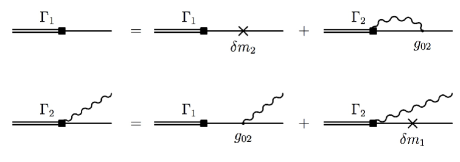
Figure 9: System of equations for the vertex functions in the two-body approximation.

Since the Hamiltonian (11) does not include contact terms, this system is much simpler than its analog considered in Ref. [7]. For simplicity, we have not drawn the lines associated with the spurion (see discussion in Appendix B). Besides that, we do not need to introduce any specific counterterms which explicitly depend on the LF plane orientation. These are evident merits of the PV regularization. The amplitudes of the LF diagrams are calculated according to the graph technique rules (see Ref. [6] and Appendix B). We denote the intermediate fermion four-momenta in the one- and two-body states as $p^{\prime}_{1i^{\prime}}$ and $k^{\prime}_{1i^{\prime}}$, respectively. The intermediate boson four-momentum is $k^{\prime}_{2j^{\prime}}$. The values of the intermediate particle momenta are defined from the conservation laws (29) in the vertices, taken for $n=1$ and $n=2$.

The system of equations reads

$$\bar{u}(p_{1i})\Gamma_{1}^{i}u(p) = \bar{u}(p_{1i})\left(V_{1}+V_{2}\right)u(p),$$ (38a)

$$\bar{u}(k_{1i})\Gamma_{2}^{ij}u(p) = \bar{u}(k_{1i})V_{3}u(p),$$ (38b)

where

$$V_{1} = \delta m_{2}\sum_{i^{\prime}}(-1)^{i^{\prime}}\frac{{\not\!p_{1i^{\prime}}^{\prime}}+m_{i^{\prime}}}{m^{2}_{i^{\prime}}-M^{2}}\Gamma_{1}^{i^{\prime}},$$ (39a)

$$V_{2} = g_{02}\int\frac{d^{2}R^{\prime}_{\perp}}{(2\pi)^{3}}\int_{0}^{1}\frac{dx^{\prime}}{2x^{\prime}(1-x^{\prime})}$$

$$\times\left[\sum_{i^{\prime},j^{\prime}}(-1)^{i^{\prime}+j^{\prime}}\frac{{\not\!k}^{\prime}_{1i^{\prime}}+m_{i^{\prime}}}{s_{12}^{i^{\prime}j^{\prime}}-M^{2}}\Gamma_{2}^{i^{\prime}j^{\prime}}\right],$$

$$V_{3} = g_{02}\sum_{i^{\prime}}(-1)^{i^{\prime}}\frac{{\not\!p^{\prime}_{1i^{\prime}}}+m_{i^{\prime}}}{m^{2}_{i^{\prime}}-M^{2}}\Gamma_{1}^{i^{\prime}},$$ (39c)

and $s_{12}^{i^{\prime}j^{\prime}}=(k^{\prime}_{1i^{\prime}}+k^{\prime}_{2j^{\prime}})^{2}$. We took into account that $\delta m_{1}=0$. Necessary kinematical relations used for deriving Eqs. (39) are given in Appendix C.1. We introduced the integration variables ${\bf R}^{\prime}_{\perp}$ and $x^{\prime}$ related to the intermediate boson momentum $k^{\prime}_{2j^{\prime}}$ in full analogy with Eqs. (37). The summations in Eqs. (39) run through 0 to 1 in each index. The system of equations (38) must be solved in the limit $M\to m$.

We have four unknown functions $b_{1}^{ij}$, four unknown functions $b_{2}^{ij}$ and two unknown constants $\psi_{1}^{i}$. So, we have to deal with a system of $10\times 10$ linear integral equations. However, Eqs. (38b) and (39c) allow to express easily $\Gamma_{2}^{ij}$ through $\Gamma_{1}^{i}$. Since $\Gamma_{1}^{i}$ are constants, it follows from these equations that $b_{1}^{ij}$ and $b_{2}^{ij}$ are constants too and they depend neither on $i$, nor on $j$. Then, due to the fact that the vertex functions come into all equations, being sandwiched with on-mass-shell bispinors, we may simply substitute $\Gamma_{2}^{ij}$ everywhere by the quantity $V_{3}$, Eq. (39c). It thus follows that we can rewrite Eq. (39) in the form, in the limit $M\to m$

$$V_{2}=-g_{02}\left.\bar{\Sigma}(p)\right|_{p^{2}=M^{2}}V_{3},$$ (40)

where

$$\bar{\Sigma}(p) = -\int\frac{d^{2}R^{\prime}_{\perp}}{(2\pi)^{3}}\int_{0}^{1}\frac{dx^{\prime}}{2x^{\prime}(1-x^{\prime})}$$ (41)

$$\times\left[\sum_{i^{\prime},j^{\prime}}(-1)^{i^{\prime}+j^{\prime}}\frac{{\not\!k_{1i^{\prime}}^{\prime}}+m_{i^{\prime}}}{s_{12}^{i^{\prime}j^{\prime}}-p^{2}}\right]$$

which is nothing else than the PV-regularized fermion two-body self-energy (apart from the coupling constant). After integration, it depends on the four-momentum $p$ only. We will use the following decomposition:

$$\bar{\Sigma}(p)\equiv{\cal A}(p^{2})+{\cal B}(p^{2})\frac{\not\!p}{m}.$$ (42)

The explicit form of the functions ${\cal A}$ and ${\cal B}$ for arbitrary values of $p^{2}$ can be found in Ref. [8].

Now, substituting Eq. (39c) into Eq. (40) and then into Eq. (38a), and using that $\Gamma_{1}^{i}=(m^{2}_{i}-M^{2})\psi_{1}^{i}$ is proportional to the unity matrix, we turn the latter equation into a system of two linear matrix equations for $\psi_{1}^{0}$ and $\psi_{1}^{1}$. Multiplying these equations by $\bar{u}(p)$ to the right and by ${u}(p_{1i})$ to the left, summarizing over the fermion polarizations, and taking the trace, we arrive at a system of two linear homogeneous equations for the one-body vertices. This system reads

$$\sum_{i^{\prime}}c^{ii^{\prime}}\psi_{1}^{i^{\prime}}=0$$ (43)

with

$$c^{00} = 8m^{2}\left\{\delta m_{2}-g_{02}^{2}(A+B)\right\},$$

$$c^{01} = -2(m+m_{1})^{2}\left\{\delta m_{2}-g_{02}^{2}(A+B)\right\},$$

$$c^{10} = 2(m+m_{1})^{2}\left\{\delta m_{2}-g_{02}^{2}(A+B)\right\},$$

$$c^{11} = \frac{(m+m_{1})^{2}}{m^{2}}\left\{m^{3}-mm_{1}\left(m_{1}+2\delta m_{2}\right)\right.$$

$$+\left.g_{02}^{2}\left[2Amm_{1}+B(m^{2}+m_{1}^{2})\right]\right\},$$

where $A={\cal A}(m^{2})$, $B={\cal B}(m^{2})$. Equating the determinant of the system to zero, we obtain a quadratic equation for $\delta m_{2}$ with the solution

$$\delta m_{2}=g_{02}^{2}(A+B).$$ (44)

The second root is rejected because it does not disappear at $g_{02}=0$. Substituting Eq. (44) into any of the two equations (43) we find

$$\psi_{1}^{0}=a_{1},\quad\psi_{1}^{1}=0,$$ (45)

where $a_{1}$ is an arbitrary constant. Substituting this solution into Eq. (39c), then into Eq. (38b), and comparing the result with the r.-h.s. of Eq. (36b), we easily obtain

$$b_{1}^{ij}=2mg_{02}a_{1},\quad b_{2}^{ij}=0.$$ (46)

It is interesting to compare the solution (45) and (46) for the one- and two-body vertex functions with that found in Ref. [7]. Due to the extension of the Fock space basis, the vertex functions considered here have more components, but both solutions possess nevertheless the same main features. Firstly, they are constants, i.e. momentum independent. Secondly, the one-body vertex has only one component: the one-body wave function of the PV fermion, $\psi_{1}^{1}$, vanishes identically, while the physical component $\psi_{1}^{0}$ is not fixed and must be computed from the normalization condition for the state vector. Thirdly, the two-body vertex has no $\omega$-dependent part, since the components $b_{2}^{ij}$ are zero. Finally, the form of the solution (46) is the same as that from Ref. [7], apart from the coupling constant which is now $g_{02}$ instead of $g$. The same is true for the MC (44).

IV.1.2 Normalization of the state vector

The Fock components found above must be properly normalized. As we have already explained, the formulas (25) and (33) for the ”partial” normalization integrals must be modified, since we have to take into account the sectors which contain PV particles. This is done very easily. One should simply sum over all possible two-body states, keeping in mind that each PV particle brings the factor $(-1)$ to the norm. The contribution of the one-body state is thus

$$I_{1} = \sum_{i}(-1)^{i}\frac{\mbox{Tr}\{({\not\!p}+m)({\not\!p}_{1i}+m_{i})\}}{2}\left(\psi_{1}^{i}\right)^{2}$$ (47)

$$= 4m^{2}\left(\psi_{1}^{0}\right)^{2}=4m^{2}a_{1}^{2}.$$

We used here Eqs. (118a) and (119) at $M=m$ from Appendix C.1. The norm of the two-body state reads

$$I_{2} = \frac{1}{2(2\pi)^{3}}\int d^{2}R_{\perp}\int_{0}^{1}\frac{dx}{2x(1-x)}\sum_{ij}(-1)^{i+j}$$ (48)

$$\times\frac{\left(b_{1}^{ij}\right)^{2}\mbox{Tr}\{({\not\!p}+m)({\not\!k}_{1i}+m_{i})\}}{(s_{12}^{ij}-m^{2})^{2}},$$

where

$$s_{12}^{ij}=\frac{R_{\perp}^{2}+\mu_{j}^{2}}{x}+\frac{R_{\perp}^{2}+m_{i}^{2}}{1-x}.$$

Substituting $b_{1}^{ij}=2m{g}_{02}a_{1}$ into Eq. (48), calculating the trace and using Eqs. (118c), (120), and (122), we obtain

$$I_{2}=\frac{m^{2}a_{1}^{2}{g}_{02}^{2}}{2\pi^{2}}\int_{0}^{\infty}dR_{\perp}\,R_{\perp}\int_{0}^{1}dx\,x\sum_{i,j}(-1)^{i+j}$$

$$\times\frac{R_{\perp}^{2}+[(1-x)m+m_{i}]^{2}}{[R_{\perp}^{2}+(1-x)\mu_{j}^{2}+xm_{i}^{2}-x(1-x)m^{2}]^{2}}.$$ (49)

Note that in order to get a finite result for $I_{2}$, the bosonic PV regularization is enough. For this reason, one can retain in the sum over $i$ the term with $i=0$ only :

$$I_{2}=4m^{2}a_{1}^{2}{g}_{02}^{2}\,J_{2},$$ (50)

where

$$J_{2} = \frac{1}{8\pi^{2}}\int_{0}^{\infty}dR_{\perp}\,R_{\perp}\int_{0}^{1}dx\,x$$ (51)

$$\times\sum_{j}\frac{(-1)^{j}[R_{\perp}^{2}+(2-x)^{2}m^{2}]}{[R_{\perp}^{2}+(1-x)\mu_{j}^{2}+x^{2}m^{2}]^{2}}.$$

From the normalization condition (24) in the two-body approximation one gets $I_{1}+I_{2}=1$ and, hence,

$$a_{1}^{2}=\frac{1}{4m^{2}(1+g_{02}^{2}J_{2})}.$$ (52)

The integral $J_{2}$ diverges logarithmically when the PV boson mass $\mu_{1}$ tends to infinity:

$$J_{2}=\frac{1}{16\pi^{2}}\log\frac{\mu_{1}}{m}+f\left(\frac{\mu}{m}\right),$$ (53)

where $f$ is a finite function independent of $\mu_{1}$. Terms vanishing in the limit $\mu_{1}\to\infty$ are neglected. Note that if $\mu_{1}$ is large enough, $J_{2}$ is positive.

The normalized one- and two-body components of the vertex functions are thus

$$\psi_{1}^{0}=\frac{1}{2m\sqrt{1+g_{02}^{2}J_{2}}},\quad\psi_{1}^{1}=0,$$ (54a)

$$b_{1}^{ij}=\frac{g_{02}}{\sqrt{1+g_{02}^{2}J_{2}}},\quad b_{2}^{ij}=0.$$ (54b)

IV.1.3 Determination of the internal bare coupling constant

According to our renormalization conditions detailed in Sec. III.2, we calculate the internal BCC $g_{02}$ from the requirement that the $\omega$-independent part of the two-body vertex function for physical particles (i.e. the component $b_{1}^{00}$), taken at $s=m^{2}$, is identified with the physical coupling constant $g$. Since in the two-body Fock space truncation $b_{1}^{ij}$ are constants, we immediately get

$$b_{1}^{00}(s=m^{2})\equiv b_{1}^{00}=\frac{g_{02}}{\sqrt{1+g_{02}^{2}J_{2}}}=g.$$ (55)

It is a well defined, non-perturbative, condition which is very convenient to impose in any numerical calculation.

From Eq. (55) it follows

$$g_{02}^{2}=\frac{g^{2}}{1-g^{2}J_{2}}.$$ (56)

The final form of the normalized (and renormalized) solution for the vertex function components becomes

$$\psi_{1}^{0}=\frac{\sqrt{1-g^{2}J_{2}}}{2m},\quad\psi_{1}^{1}=0,$$ (57a)

$$b_{1}^{ij}=g,\quad b_{2}^{ij}=0.$$ (57b)

The one- and two-body contributions to the norm of the state vector are

$$I_{1}=1-g^{2}J_{2},\quad I_{2}=g^{2}J_{2}.$$ (58)

As we said above, if $\mu_{1}$ increases, the quantity $J_{2}$ increases too. At some value of $\mu_{1}$ we inevitably meet the condition $g^{2}J_{2}=1$, leading to a pole on the r.-h.s. of Eq. (56), analogous to the well-known Landau pole in QED. Further increase of $\mu_{1}$ makes $g_{02}^{2}$ negative and $g_{02}$ purely imaginary [as well as $\psi_{1}^{0}$, Eq. (54a)]. At the same time, the one- and two-body norms $I_{1}$ and $I_{2}$ become infinitely large, but have opposite signs: $I_{1}$ is negative, while $I_{2}$ is positive. So one can not get rid at this level of the regularization parameters by taking the limit $\mu_{1}\to\infty$ without formal contradiction. A possible way out is as follows. The PV masses play an auxiliary role and appear in intermediate calculations only, while physical observables must be independent of them (the BCC $g_{02}$ is not an observable!). We do not give any physical interpretation to intermediate results found with finite PV masses. Below we will treat $J_{2}$ as being a finite quantity satisfying the inequality $1-g^{2}J_{2}>0$ (formally, this can be done by proper adjustment of the value of $\mu_{1}$). Then, we express the calculated Fock components through the physical coupling constant, normalize the state vector, calculate the observables, and after that go over to the limit of infinite PV masses in the final result. We will demonstrate below how this scheme works in practice.

IV.1.4 Determination of the external bare coupling constant

To determine the external BCC one has to consider the 3PGF, denoted by $G$, which is represented, in the two-body approximation, by a sum of the two contributions shown in Fig. 10. Similarly to the two-body vertex function (36b), the 3PGF can be decomposed in invariant amplitudes:

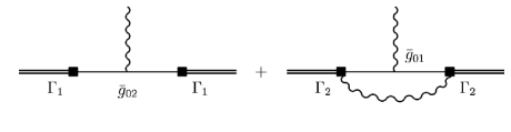
Figure 10: Fermion-boson 3PGF in the two-body approximation.

$$\bar{u}(p^{\prime})Gu(p)=g\bar{u}(p^{\prime})\left(F+B_{\omega}\frac{m\not\!\omega}{\omega\makebox[2.27626pt]{$\cdot$}p}\right)u(p).$$ (59)

The invariant functions $F$ and $B_{\omega}$ (scalar form factors) depend, under the condition $\omega\makebox[2.27626pt]{$\cdot$}q=0$, on $q^{2}\equiv(p^{\prime}-p)^{2}$. Note that the general decomposition (59) in the Yukawa model is valid in any approximation, since the number of independent invariant amplitudes is completely determined by particle spins and by symmetries of the interaction. The external BCC is found from the requirement

$$\bar{u}(p^{\prime})Gu(p)=g\bar{u}(p^{\prime})u(p)\quad\mbox{at}\quad q^{2}=\mu^{2}.$$ (60)

Hence, we must have $F(q^{2}=\mu^{2})=1$ and $B_{\omega}(q^{2}=\mu^{2})=0$. In exact calculations, as well as in a given order of perturbation theory, we would indeed get $B_{\omega}\equiv 0$, because physical amplitudes can not depend on the LF plane orientation. In approximate non-perturbative calculations however it may turn out that $B_{\omega}$ does not disappear, even at $q^{2}=\mu^{2}$. Then, according to our renormalization prescriptions, one should add to the LF Hamiltonian the counterterm

$$Z_{3}\bar{\psi}\frac{m\not\!\omega}{i\omega\makebox[2.27626pt]{$\cdot$}\partial}\psi\varphi\ .$$

The structure of the counterterm is the same in all approximations, while the constant $Z_{3}$ must depend on the Fock sector, in complete analogy with the BCC’s. We therefore have to calculate both $Z_{3l}$ (for internal coupling) and $\bar{Z}_{3l}$ (for external coupling). In the particular case discussed here, i.e for the two-body Fock space truncation with the use of the PV regularization (with one PV boson and one PV fermion), we find $B_{\omega}=0$. We therefore get $\bar{Z}_{31}=\bar{Z}_{32}=Z_{31}=Z_{32}=0$.

We will now concentrate on the calculation of the physical scalar form factor $F$. It can be extracted from the 3PGF by the relation

$$gF=\frac{1}{2q^{2}}\,\mbox{Tr}\left[({\not\!p}^{\prime}+m)G({\not\!p}+m)\left(\frac{m{\not\!\omega}}{\omega\makebox[2.27626pt]{$\cdot$}p}-1\right)\right].$$ (61)

First, we calculate $F$, as a function of $q^{2}$, for physical values $q^{2}\leq 0$ and then find its analytical continuation to the non-physical point $q^{2}=\mu^{2}$.

In the two-body approximation, the 3PGF can be represented as

$$G\equiv\bar{g}_{02}\bar{G}_{1}+\bar{g}_{01}\bar{G}_{2},$$ (62)

where $\bar{G}_{1,2}$ denote the contributions (amputated from the external BCC’s) to the full 3PGF from the one- and two-body sectors, respectively. Applying the CLFD graph technique rules to the diagrams shown in Fig. 10, we have

$$\bar{G}_{1} = \sum_{i,i^{\prime}}(-1)^{i+i^{\prime}}\psi_{1}^{i}\psi_{1}^{i^{\prime}}\left[({\not\!p}^{\prime}+{\not\!\omega}\tau_{1}^{\prime}+m_{i^{\prime}})\right.$$ (63a)

$$\times\left.({\not\!p}+{\not\!\omega}\tau_{1}+m_{i})\right],$$

$$\bar{G}_{2} = \frac{1}{(2\pi)^{3}}\int d^{2}R_{\perp}\int_{0}^{1}\frac{dx}{2x}\sum_{i,i^{\prime},j}(-1)^{i+i^{\prime}+j}$$ (63b)

$$\times\frac{\bar{\Gamma}_{2}^{i^{\prime}j}({\not\!p}^{\prime}-{\not\!k}_{2j}+{\not\!\omega}\tau_{2}^{\prime}+m_{i^{\prime}})}{(p^{\prime}-k_{2j})^{2}-m_{i^{\prime}}^{2}}$$

$$\times\frac{({\not\!p}-{\not\!k}_{2j}+{\not\!\omega}\tau_{2}+m_{i})\Gamma_{2}^{ij}}{(p-k_{2j})^{2}-m_{i}^{2}},$$

where the variables $x$ and ${\bf R}_{\perp}$ are defined by Eqs. (37), and $\tau$’s are given by Eqs. (119), (122), and (123) taken for $M=m$. Kinematical relations needed to express the scalar products of the four-momenta through $x$ and ${\bf R}_{\perp}$ can be found in Appendix C.2. To make the integral in Eq. (63b) convergent, it is enough to regularize it by the bosonic PV subtraction only, as we did for the calculation of $J_{2}$ in Eq. (51). We can thus neglect in the sum the terms with either $i$ or $i^{\prime}$ being 1. According to the solution (57b) for the two-body component of the state vector, $\Gamma_{2}^{ij}=b_{1}^{ij}=g$. Using the solution (57a) for the one-body component, substituting Eqs. (63a) and (63b) into Eq. (62) and then into Eq. (61), we find

$$gF=\bar{g}_{02}{\cal F}^{(1)}+\bar{g}_{01}{\cal F}^{(2)}(q^{2}),$$ (64)

where

$${\cal F}^{(1)} = 1-g^{2}J_{2},$$ (65a)

$${\cal F}^{(2)}(q^{2}) = \frac{g^{2}}{16\pi^{3}}\int d^{2}R_{\perp}\int_{0}^{1}dx\sum_{j}\frac{(-1)^{j}x[2({\bf R}_{\perp}{\mbox{\boldmath$\Delta$}})^{2}/\Delta^{2}-R_{\perp}^{2}-x{\bf R}_{\perp}{\mbox{\boldmath$\Delta$}}+(3x^{2}-8x+4)m^{2}]}{(1-x)[R_{\perp}^{2}+(1-x)\mu_{j}^{2}+x^{2}m^{2}][({\bf R}_{\perp}-x{\mbox{\boldmath$\Delta$}})^{2}+(1-x)\mu_{j}^{2}+x^{2}m^{2}]}$$

with ${\mbox{\boldmath$\Delta$}}={\bf q}_{\perp}$ and $\Delta^{2}=-q^{2}$. The functions ${\cal F}^{(1)},{\cal F}^{(2)}$ determine the contributions to the scalar form factor $F$ from the one- and two-body Fock sectors. The integration over $d^{2}R_{\perp}$ in Eq. (65) can be performed analytically and leads to the result

$${\cal F}^{(2)}(q^{2})=\frac{g^{2}}{4\pi^{2}\sqrt{-q^{2}}}\int_{0}^{1}dx\sum_{j}(-1)^{j}$$

$$\times\frac{[4(1-x)m^{2}+\mu_{j}^{2}]}{r_{j}(q^{2})}\,\log\left[\frac{x\sqrt{-q^{2}}+r_{j}(q^{2})}{2\sqrt{x^{2}m^{2}+(1-x)\mu_{j}^{2}}}\right],$$ (66)

where

$$r_{j}(q^{2})=\sqrt{x^{2}(4m^{2}-q^{2})+4(1-x)\mu_{j}^{2}}.$$

According to Eq. (35b), $\bar{g}_{01}=g$, and Eq. (64) contains one unknown parameter, namely, the external BCC $\bar{g}_{02}$ which is found from the renormalization condition $F(q^{2}=\mu^{2})=1$. We thus get

$$g=\bar{g}_{02}(1-g^{2}J_{2})+g{\cal F}^{(2)}(\mu^{2}),$$ (67)

where $J_{2}$ is defined by Eq. (53) and

$${\cal F}^{(2)}(\mu^{2})=\frac{g^{2}}{4\pi^{2}\mu}\int_{0}^{1}dx\sum_{j}(-1)^{j}$$

$$\times\frac{[4(1-x)m^{2}+\mu_{j}^{2}]}{r_{j}(\mu^{2})}\arctan\left[\frac{\mu x}{r_{j}(\mu^{2})}\right].$$ (68)

The asymptotic value of ${\cal F}^{(2)}(\mu^{2})$ at $\mu_{1}\to\infty$ is

$${\cal F}^{(2)}(\mu^{2})=-\frac{g^{2}}{8\pi^{2}}\log\frac{\mu_{1}}{m}+g^{2}f_{1}\left(\frac{\mu}{m}\right),$$ (69)

where $f_{1}$ is a function of the ratio $\mu/m$, finite at $\mu_{1}\to\infty$. Substituting Eqs. (69) and (53) into Eq. (67), we find for the external BCC:

$$\bar{g}_{02}=g\,\frac{{\displaystyle 1+\frac{g^{2}}{8\pi^{2}}\log\frac{\mu_{1}}{m}-g^{2}f_{1}\left(\frac{\mu}{m}\right)}}{{\displaystyle 1-\frac{g^{2}}{16\pi^{2}}\log\frac{\mu_{1}}{m}-g^{2}f\left(\frac{\mu}{m}\right)}}.$$ (70)

The internal and external BCC’s given by Eqs. (56) and (70), respectively, differ from each other. We have already mentioned in Sec. III.1.2 that they indeed should not coincide. We can illustrate the origin of this difference in a very clear form, by analyzing contributions to the internal and external BCC’s from various LF diagrams taken into account in our calculations. Since $g_{02}$ and $\bar{g}_{02}$ differ already at order $g^{2}$ of their perturbative expansions, it is enough, to clarify the situation, to consider the lowest order perturbative corrections to BCC’s. They are indicated in Fig. 11 where the outgoing wavy line corresponds to an external boson. As it has been pointed out above, only the diagrams (a) and (b) are incorporated when calculating the internal BCC $g_{02}$ in the two-body approximation. Concerning the external BCC $\bar{g}_{02}$, the diagrams (c), (d), and (e) are included in addition, though they formally correspond to a three-body state admixture, with the external field. In other words, our calculation of $\bar{g}_{02}$ is effectively performed to higher order approximation, than that of $g_{02}$. One may expect that increasing the number of Fock components involved into calculations will reduce the difference between the internal and external BCC’s.

The diagram (f) in Fig. 11, containing the fermion-antifermion pair intermediate state, does not contribute, in the two-body approximation, neither to $g_{02}$ nor to $\bar{g}_{02}$. For this reason, both BCC’s, even being expanded in powers of $g$ up to terms of order $g^{2}$, differ from the BCC found in the second order of perturbation theory.

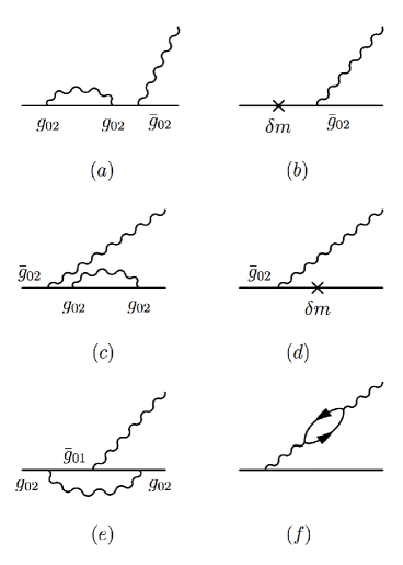
Figure 11: Second order perturbative corrections to the internal and external BCC’s.

As follows from Eqs. (64) and (67), the scalar form factor $F$ is given by

$$F=1+{\cal F}^{(2)}(q^{2})-{\cal F}^{(2)}(\mu^{2}).$$ (71)

It is easy to see that the expression on the r.-h.s. is finite in the limit $\mu_{1}\to\infty$, though each of the functions ${\cal F}^{(2)}$ diverges logarithmically. Eq. (71) coincides with the result of the 3PGF renormalization in the second order of perturbation theory, in spite of the fact that we did not make any expansion in powers of the coupling constant.

IV.2 Application to QED

IV.2.1 Determination of the state vector

The Yukawa model considered in the previous section is a good example of how the general renormalization scheme developed in this article should be understood. We will now apply the method to QED in order to address the case of a realistic physical theory. The perturbative approach to QED was able to reproduce multiple experimental data with excellent precision. Applying the non-perturbative scheme to the same object gives us a possibility to test our results and to reveal distinctly its main differences, as compared to perturbation theory.

From a purely technical point of view, QED is more complicated than the Yukawa model, at least, in the following three aspects. Firstly, the structure of the interaction Hamiltonian in QED is more involved than that in the case of scalar bosons. The consideration of QED within CLFD, performed in Ref. [7], showed that the corresponding Hamiltonian (obtained without introducing PV fields) contained specific contact terms, different from those which appear in the Yukawa model. It is not yet clear whether PV fields can kill the contact terms in this case. Secondly, many-body wave functions in QED have more spin components than their counterparts in the Yukawa model. Thirdly, intermediate calculations in QED essentially depend on the gauge condition to constrain the electromagnetic field, while the question how the Fock space truncation affects gauge invariance is still opened.

The difficulties of treating QED in the framework of CLFD, itemized above, are however absent for the two-body Fock space truncation. In this approximation, QED and the Yukawa model are very close to each other. We repeat below the procedure of finding the state vector and its renormalization, detailed in Sec. IV.1, for QED in the two-body truncated Fock space. Because of similarities between QED and the Yukawa model, we will not expose all the steps, but concentrate on pointing out the differences and demonstrating the main results of our analysis.

The general structure of the two-body electron-photon vertex function in QED has been extensively studied in Ref. [7]. For the case of the simple two-body Fock space truncation, the interaction Hamiltonian in the Feynman gauge is very similar to that in the Yukawa model, with the scalar vertex being replaced by the electromagnetic one. Provided the PV regularization is used, with one PV boson and one PV fermion, the fermion self-energy does not depend on the LF plane orientation.

According to Ref. [7], the state vector has the following structure:

$$\bar{u}(p_{1i})\Gamma_{1}^{i}u(p)=(m_{i}^{2}-M^{2})\psi_{1}^{i}\bar{u}(p_{1i})u(p),$$ (72a)

$$\bar{u}(k_{1i})\left[\Gamma_{2}^{ij,\nu}e_{\nu}^{\lambda}(k_{2j})\right]u(p)\\ =\bar{u}(k_{1i})\left[b_{1}^{ij}\gamma^{\nu}+b_{2}^{ij}{\displaystyle\frac{m{\omega^{\nu}}}{\omega\makebox[2.27626pt]{$\cdot$}p}}\right]e_{\nu}^{\lambda}(k_{2j})u(p),$$ (72b)

where $e_{\nu}^{\lambda}(k_{2j})$ is the photon polarization vector. The scalar functions $\psi_{1}^{i}$, $b_{1}^{ij}$, and $b_{2}^{ij}$ differ, generally speaking, from those entering Eqs. (36). The decomposition (72b) with the two matrix components is valid only within the two-body Fock space truncation. The number of independent components of the two-body vertex function in QED depends on the gauge. If the Feynman gauge is chosen, there are eight independent components in the general case. Under the two-body approximation, six of them identically turn into zero.

The system of equations for the QED vertex functions is very close to that for the Yukawa model, shown in Fig. 9 and given analytically by Eqs. (38) and (39). Small changes are required, caused by the vector character of the photon. Namely, one has to substitute $g_{02}\to e_{02}\gamma^{\rho}$, $\Gamma_{2}^{ij}\to\Gamma_{2}^{ij,\nu}$, and $\bar{\Sigma}(p)\to\bar{\Sigma}_{\rho\nu}(p)$, where, in the Feynman gauge,

$$\bar{\Sigma}_{\rho\nu}(p)=-g_{\rho\nu}\left[{\cal A}(p^{2})+{\cal B}(p^{2})\frac{\not\!p}{m}\right].$$ (73)

The scalar functions ${\cal A}$ and ${\cal B}$ here differ from those in Eq. (42). They were calculated (for the longitudinal and transversal LFD cutoffs) in Ref. [7]. We do not need to know their explicit form in the following.

The technical procedure to solve the system of equations for the vertex functions is exactly the same as in Sec. IV.1.1. The solution looks as follows:

$$\delta m_{2}=2e_{02}^{2}(2A-B),$$ (74)

with $A={\cal A}(m^{2})$, $B={\cal B}(m^{2})$, and

$$\psi_{1}^{0}=a_{1},\quad\psi_{1}^{1}=0,$$ (75a)

$$b_{1}^{ij}=2me_{02}a_{1},\quad b_{2}^{ij}=0.$$ (75b)

Eqs. (75a) and (75b) coincide in form with Eqs. (45) and (46), respectively. The constant $a_{1}$ is found from the normalization condition.

IV.2.2 Normalization of the state vector

The calculation of the one- and two-body normalization integrals is analogous to that for the Yukawa model. The one-body integral is exactly the same as in Eq. (47), since it is not sensitive to the boson type. The two-body integral is different:

$$I_{2}=4m^{2}a_{1}^{2}{e}_{02}^{2}\,\tilde{J}_{2},$$ (76)

where

$$\tilde{J}_{2} = \frac{1}{4\pi^{2}}\int_{0}^{\infty}dR_{\perp}\,R_{\perp}\int_{0}^{1}dx\,x$$ (77)

$$\times\sum_{j}\frac{(-1)^{j}[R_{\perp}^{2}+(x^{2}+2x-2)m^{2}]}{[R_{\perp}^{2}+(1-x)\mu_{j}^{2}+x^{2}m^{2}]^{2}}.\quad$$

The integral $\tilde{J}_{2}$ at $\mu_{1}\to\infty$ diverges logarithmically, as $J_{2}$ in the Yukawa model [see Eq. (53)], but with a different coefficient at the logarithm:

$$\tilde{J}_{2}=\frac{1}{8\pi^{2}}\log\frac{\mu_{1}}{m}-\frac{1}{4\pi^{2}}\left(\log\frac{m}{\lambda}-\frac{9}{8}\right),$$ (78)

where we assigned a finite (small) mass $\lambda$ to the photon in order to avoid the infra-red catastrophe. Note that $\tilde{J}_{2}$ is positive in the limit of infinite PV boson mass.

The normalized solution is given by Eqs. (54), changing $g_{02}$ by $e_{02}$ and $J_{2}$ by $\tilde{J}_{2}$.

IV.2.3 Determination of the internal bare coupling constant

Due to the formal coincidence of the state vector structures in the Yukawa model and QED, we immediately obtain from Eq. (56):

$$e_{02}^{2}=\frac{e^{2}}{1-e^{2}\tilde{J_{2}}}.$$ (79)

The final solution for the vertex function components is

$$\psi_{1}^{0}=\frac{\sqrt{1-e^{2}\tilde{J}_{2}}}{2m} \quad\psi_{1}^{1}=0,$$ , (80a)

$$b_{1}^{ij}=e \quad b_{2}^{ij}=0.$$ , (80b)

It is in full analogy with the corresponding solution for the state vector in the Yukawa model, given by Eqs. (57).

IV.2.4 Determination of the external bare coupling constant and calculation of the electromagnetic form factors

We will establish in this section the relationship between the external electromagnetic BCC and the physical fermion charge and compute the fermion electromagnetic form factors in the two-body approximation. The main difference, as compared to the electromagnetic interaction with a system formed by the Yukawa interaction, consists in the fact that now the photon emitted (or absorbed) by the probe is of the same type as photons coming into the state vector. Formally speaking, the right diagram in Fig. 10 contains a three-body intermediate state and must be rejected. However, according to our renormalization scheme detailed in Sec. III.1.2, one should treat the photon connecting the electromagnetic vertex with the probe as if it was an external particle, having no relation to the contents of the state vector. This makes possible the calculation of non-trivial observables already within the two-body approximation.

In CLFD, the spin-1/2 fermion 3PGF (or electromagnetic vertex, i.e. the current matrix element between the initial and final fermion states) has the following general structure [21, 8] (we have included the physical electromagnetic coupling constant $e$ into the definition of the vertex):

$$\bar{u}(p^{\prime})G^{\rho}u(p)=e\bar{u}(p^{\prime})\left[F_{1}\gamma^{\rho}+\frac{iF_{2}}{2m}\sigma^{\rho\nu}q_{\nu}+B_{1}\left(\frac{{\not\!\omega}}{\omega\makebox[2.27626pt]{$\cdot$}p}P^{\rho}-2\gamma^{\rho}\right)+B_{2}\frac{m{\omega^{\rho}}}{\omega\makebox[2.27626pt]{$\cdot$}p}+B_{3}\frac{m^{2}{\not\!\omega}\omega^{\rho}}{(\omega\makebox[2.27626pt]{$\cdot$}p)^{2}}\right]u(p)$$ (81)

with $\sigma^{\rho\nu}=i(\gamma^{\rho}\gamma^{\nu}-\gamma^{\nu}\gamma^{\rho})/2$ and $P=p^{\prime}+p$. It is determined by five form factors, the two physical ($F_{1,2}$) and the three non-physical ($B_{1-3}$) ones. The non-physical form factors are coefficients at the spin structures which depend on $\omega$. The term proportional to $B_{1}$ is constructed in such a way that it gives zero when sandwished between free spinors of momentum $p^{\prime}=p$. It gives also zero when contracted with $\omega_{\rho}$. Under the condition $\omega\makebox[2.27626pt]{$\cdot$}q=0$ the form factors depend on $Q^{2}=-q^{2}$. If the electromagnetic vertex is calculated exactly or within a given order of perturbation theory and, moreover, is regularized in a rotationally invariant way, the non-physical form factors cancel identically, while the two physical form factors remain, as it should be. Under approximate non-perturbative calculations, the non-physical form factors may however survive and plague the electromagnetic vertex by spurious $\omega$-dependent contributions. The situation here is fully analogous to that for the Yukawa model, where the function $B_{\omega}$ in Eq. (59) is just a non-physical scalar form factor. CLFD allows to separate covariantly the physical and non-physical parts of the electromagnetic vertex and extract the physical form factors from the former. In our case, it is enough to contract both sides of Eq. (81) with the four-vector $\omega_{\rho}$:

$$\bar{u}(p^{\prime})\omega_{\rho}G^{\rho}u(p)=e\bar{u}(p^{\prime})\left[F_{1}{\not\!\omega}+\frac{iF_{2}}{2m}\sigma^{\rho\nu}\omega_{\rho}q_{\nu}\right]u(p).$$ (82)

As we see, the three non-physical form factors $B_{1-3}$ disappeared, since the contraction of the spin structures proportional to them with $\omega_{\rho}$ gives zero. The physical form factors can be found by the following expressions:

$$eF_{1}=\frac{\mbox{Tr}[({\not\!p}^{\prime}+m)\omega_{\rho}G^{\rho}({\not\!p}+m){\not\!\omega}]}{8(\omega\makebox[2.27626pt]{$\cdot$}p)^{2}},\\$$ (83a)

$$eF_{2}=\frac{m}{2(\omega\makebox[2.27626pt]{$\cdot$}p)Q^{2}}\\ \times\mbox{Tr}\left[({\not\!p}^{\prime}+m)\omega_{\rho}G^{\rho}({\not\!p}+m)\left(\frac{m{\not\!\omega}}{\omega\makebox[2.27626pt]{$\cdot$}p}-1\right)\right].$$ (83b)

Similarly to Eq. (62), we write

$$\omega_{\rho}G^{\rho}\equiv\bar{e}_{02}\bar{G}_{1}+\bar{e}_{01}\bar{G}_{2},$$ (84)

where

$$\bar{G}_{1}=\sum_{i,i^{\prime}}(-1)^{i+i^{\prime}}\psi_{1}^{i}\psi_{1}^{i^{\prime}}\left[({\not\!p}^{\prime}+m_{i^{\prime}}){\not\!\omega}({\not\!p}+m_{i})\right],$$ (85a)

$$\bar{G}_{2}=-\frac{1}{(2\pi)^{3}}\int d^{2}R_{\perp}\int_{0}^{1}\frac{dx}{2x}\sum_{i,i^{\prime},j}(-1)^{i+i^{\prime}+j}\\ \times\frac{\bar{\Gamma}_{2}^{i^{\prime}j,\nu}({\not\!p}^{\prime}-{\not\!k}_{2j}+m_{i^{\prime}}){\not\!\omega}({\not\!p}-{\not\!k}_{2j}+m_{i})\Gamma_{2}^{ij,\nu}}{[(p^{\prime}-k_{2j})^{2}-m_{i^{\prime}}^{2}][(p-k_{2j})^{2}-m_{i}^{2}]}.$$ (85b)

Again, to make the integral in Eq. (85b) convergent, it is enough to regularize it by the bosonic PV subtraction only. We can thus retain in the sum the term with $i=i^{\prime}=0$, neglecting those with either $i$ or $i^{\prime}$ equal to 1. According to the solution (80b) for the two-body component of the state vector, $\Gamma_{2}^{ij,\nu}=b_{1}^{ij}\gamma^{\nu}=e\gamma^{\nu}$. Using the solution (80a) for the one-body component, substituting Eqs. (85) into Eq. (84) and then into each of Eqs. (83), we find

$$eF_{1} = \bar{e}_{02}{\cal F}_{1}^{(1)}+\bar{e}_{01}{\cal F}_{1}^{(2)}(Q^{2}),$$ (86a)

$$eF_{2} = \bar{e}_{01}{\cal F}_{2}^{(2)}(Q^{2}),$$ (86b)

where $\bar{e}_{01}=e$,

$${\cal F}_{1}^{(1)}=1-e^{2}\tilde{J}_{2},$$ (87)

$\tilde{J}_{2}$ is given by Eq. (77), and

$${\cal F}_{1}^{(2)}(Q^{2}) = \frac{e^{2}}{8\pi^{3}}\int d^{2}R_{\perp}$$

$$\int_{0}^{1}dx\sum_{j}\frac{(-1)^{j}x[R_{\perp}^{2}-x{\bf R}_{\perp}{\mbox{\boldmath$\Delta$}}+(x^{2}+2x-2)m^{2}-(1-x){\Delta}^{2}]}{[R_{\perp}^{2}+(1-x)\mu_{j}^{2}+x^{2}m^{2}][({\bf R}_{\perp}-x{\mbox{\boldmath$\Delta$}})^{2}+(1-x)\mu_{j}^{2}+x^{2}m^{2}]},$$

$${\cal F}_{2}^{(2)}(Q^{2}) = \frac{e^{2}m^{2}}{4\pi^{3}}\int d^{2}R_{\perp}$$

$$\int_{0}^{1}dx\sum_{j}\frac{(-1)^{j}x^{2}(1-x)}{[R_{\perp}^{2}+(1-x)\mu_{j}^{2}+x^{2}m^{2}][({\bf R}_{\perp}-x{\mbox{\boldmath$\Delta$}})^{2}+(1-x)\mu_{j}^{2}+x^{2}m^{2}]}.$$

Here $\mu_{0}\equiv\mu=0$. Note that ${\cal F}_{1}^{(2)}(0)=e^{2}\tilde{J}_{2}$ which is just the norm of the two-body sector.

The requirement $F_{1}=1$ at $Q^{2}=0$ leads to the relation

$$eF_{1}(Q^{2}=0)\equiv e=\bar{e}_{02}(1-e^{2}\tilde{J}_{2})+e^{3}\tilde{J}_{2},$$ (89)

so that

$$\bar{e}_{02}=e.$$ (90)

Hence, the electromagnetic external BCC calculated in the two-body approximation is not renormalized. Such a coincidence happens not by chance, but reflects a general property of the theory. We will discuss this fact in more detail below.

From Eqs (86) we find the renormalized form factors:

$$F_{1} = 1+{\cal F}_{1}^{(2)}(Q^{2})-{\cal F}_{1}^{(2)}(0),$$ (91a)

$$F_{2} = {\cal F}_{2}^{(2)}(Q^{2}).$$ (91b)

This result exactly coincides with that found in the second order of perturbation theory, though no expansions in the coupling constant have been done. A similar issue was obtained above for the Yukawa model [see Eq. (71)].

Expressing $e^{2}$ through the fine structure constant $\alpha$ by the relation $e^{2}=4\pi\alpha$ and calculating the integrals (88), we obtain (for simplicity, we decomposed the form factors in powers of $Q^{2}$, up to second order):

$$F_{1} = 1-\frac{\alpha Q^{2}}{3\pi m^{2}}\left(\log\frac{m}{\lambda}-\frac{3}{8}\right)+O(Q^{4}),\quad$$ (92a)

$$F_{2} = \frac{\alpha}{2\pi}-\frac{\alpha Q^{2}}{12\pi m^{2}}+O(Q^{4}).$$ (92b)

The formulas (92) exactly coincide with the familiar perturbative expressions. In particular, $F_{2}$ at $Q^{2}=0$ reproduces the well-known Schwinger correction [22] to the electron anomalous magnetic moment. As expected, the form factors have finite limits, when the PV masses tend to infinity.

The external and internal BCC’s calculated in the two-body approximation and given, respectively, by Eqs. (90) and (79) do not coincide, as in the Yukawa model. This fact has been already explained in the end of Sec. IV.1.4. In QED however, we encounter a new effect, namely, the identity between the external BCC $\bar{e}_{02}$ and the physical electron charge $e$. It is a specific feature of QED, which appears as a consequence of the Ward identity. To illustrate the situation, one may come back to Fig. 11. Due to the Ward identity, the total contribution of the perturbative diagrams (a)–(e) gives zero, and the external BCC ${\bar{e}}_{02}$ is not renormalized at all. The same arguments hold true for the non-perturbative calculations in two-body truncated Fock space. As we will see in the next section, this takes place for truncations of any order.

One more point is also worth mentioning. Neither the perturbative expansion of the internal BCC, Eq. (79), at $\mu_{1}\to\infty$,

$$e_{02}^{2}=e^{2}\left(1+\frac{\alpha}{4\pi}\log\frac{\mu_{1}^{2}}{m^{2}}\right),$$

nor the external BCC $\bar{e}_{02}^{2}=e^{2}$ coincide with the well-known purely perturbative formula relating the BCC with the physical charge and given in most textbooks on quantum field theory:

$$e_{0,pert}^{2}=e^{2}\left(1+\frac{\alpha}{3\pi}\log\frac{\Lambda^{2}}{m^{2}}\right),$$ (93)

where $\Lambda^{2}$ is an invariant cutoff which can be identified, in the logarithmic approximation, with $\mu_{1}^{2}$. This result is nevertheless quite natural, since Eq. (93), besides the contributions shown in Fig. 11(a-e) (which, being summed up, give zero due to the Ward identity), takes into account also the effect of vacuum polarization, i.e. the diagram with the electron-positron loop on the external photon line, shown in Fig. 11(f). Evidently, our two-body approximation is unable to embrace such an effect. The latter can be incorporated when Fock sectors containing electron-positron pairs are included into the state vector.

IV.2.5 External bare coupling constant. What happens for $N>2$ ?

We can easily generalize the result (90) to the case where an arbitrary number of photons in the state vector is considered. We can do that by recurrence. In the $N=3$ case (one electron and no more than two photons), for instance, the form factors are given by the contributions from the diagrams shown in Fig. 12.

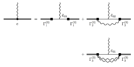
Figure 12: Electron electromagnetic vertex for the three-body Fock space truncation.

At $Q^{2}=0$ we have

$$e=\bar{e}_{03}{\cal F}_{1}^{(1)}+\bar{e}_{02}{\cal F}_{1}^{(2)}(Q^{2}=0)+\bar{e}_{01}{\cal F}_{1}^{(3)}(Q^{2}=0).$$ (94)

The functions ${\cal F}_{1}^{(1,2,3)}$ are just the contributions of the amplitudes of the three diagrams on the r.-h.s. of the graphical equation shown in Fig. 12. For QED, one can easily check that ${\cal F}_{1}^{(n)}(Q^{2}=0)=I_{n}$, where $I_{n}$ is the contribution of the $n$-body Fock sector to the norm of the state vector. With $\bar{e}_{01}=\bar{e}_{02}=e$ we get

$$e=\bar{e}_{03}I_{1}+e(I_{2}+I_{3}).$$ (95)

Due to the normalization condition, $I_{1}+I_{2}+I_{3}=1$. We thus have

$$e=\bar{e}_{03}\left[1-(I_{2}+I_{2})\right]+e(I_{2}+I_{3}),$$ (96)

so that

$$\bar{e}_{03}=e.$$ (97)

Repeating the same arguments to the cases of $N=4,\,5,\ldots$ Fock space truncations, we conclude that Eq. (97) holds to all orders in $N$. Hence, our formalism respects the requirement of the Ward identity even in truncated Fock space.

V Application to the N=3 Fock space truncation in a scalar model

We re-examine here our previous calculation [20] of the state vector in a pure scalar model for the three-body Fock space truncation, using the renormalization strategy outlined above. We shall see how this strategy should be applied in the context of a non-perturbative physical problem where the results can not be reproduced in perturbation theory, unlike the cases of the two-body approximation in the Yukawa model and QED.

Though all the particles we consider are spinless, we will distinguish two types of them, described by the free fields $\varphi(x)$ and $\chi(x)$ and related to the ”main” (i.e. analogous to fermions in the Yukawa model or QED) and ”exchanged” particles. For shortness, we will refer to them as scalar ”nucleons” and bosons, respectively. The interaction Hamiltonian is

$$H^{int}(x)=-g_{0}\varphi^{2}\chi^{\prime}-\delta m^{2}\varphi^{2},$$ (98)

where the prime at $\chi$ denotes the fact that it is a sum of a physical and a PV component. Since all divergencies are regularized already by the PV boson, we do not need to introduce a PV ”nucleon”. The Hamiltonian (98) contains the BCC $g_{0}$ and the MC $\delta m^{2}$ which must be adjusted to reproduce correctly the physical ”nucleon” mass $m$ and the physical coupling constant $g$.

The system of eigenstate equations for the vertex functions in the three-body approximation is shown graphically in Fig. 13. Solid and wavy lines correspond to ”nucleons” and bosons. In analytical form the system of equations reads

$$\Gamma_{1} = \frac{\delta m_{3}^{2}\Gamma_{1}}{m^{2}-M^{2}}+g_{03}\sum_{j}\frac{(-1)^{j}}{(2\pi)^{3}}\int d^{2}R_{\perp}\int_{0}^{1}\frac{dx}{2x(1-x)}\,\frac{\Gamma_{2}^{j}(R_{\perp},x)}{s_{12}^{j}-M^{2}},$$ (99a)

$$\Gamma_{2}^{j}(R_{\perp},x) = \frac{g_{03}\Gamma_{1}}{m^{2}-M^{2}}+\frac{\delta m_{2}^{2}\Gamma_{2}^{j}(R_{\perp},x)}{(1-x)(s_{12}^{j}-M^{2})}$$ (99b)

$$+g_{02}\sum_{j^{\prime}}\frac{(-1)^{j^{\prime}}}{(2\pi)^{3}}\int d^{2}R^{\prime}_{\perp}\int_{0}^{1-x}dx^{\prime}\frac{\Gamma_{3}^{jj^{\prime}}({R}_{\perp},x;{R}^{\prime}_{\perp},x^{\prime})}{2x^{\prime}(1-x-x^{\prime})(s_{123}^{jj^{\prime}}-M^{2})},$$

$$\Gamma_{3}^{jj^{\prime}}(R_{\perp},x;R^{\prime}_{\perp},x^{\prime}) = \frac{g_{02}\Gamma_{2}^{j}(R_{\perp},x)}{(1-x)(s_{12}^{j}-M^{2})}+\frac{g_{02}\Gamma_{2}^{j^{\prime}}(R^{\prime}_{\perp},x^{\prime})}{(1-x^{\prime})(s_{13}^{j^{\prime}}-M^{2})}$$ (99c)

with

$$s_{12}^{j} = \frac{R_{\perp}^{2}+m^{2}}{(1-x)}+\frac{R_{\perp}^{2}+\mu^{2}_{j}}{x},$$

$$s_{13}^{j^{\prime}} = \frac{{R^{\prime}}_{\perp}^{2}+m^{2}}{(1-x^{\prime})}+\frac{{R^{\prime}}_{\perp}^{2}+\mu^{2}_{j^{\prime}}}{x^{\prime}},$$

$$s_{123}^{jj^{\prime}} = \frac{({\bf R}_{\perp}+{\bf R}^{\prime}_{\perp})^{2}+m^{2}}{(1-x-x^{\prime})}+\frac{R_{\perp}^{2}+\mu^{2}_{j}}{x}+\frac{{R^{\prime}}_{\perp}^{2}+\mu^{2}_{j^{\prime}}}{x^{\prime}}.$$

In deriving Eqs. (99) we took into account that $\delta m_{1}^{2}=0$, since no ”nucleon” mass renormalization occurs for the one-body Fock space truncation. As before, the index $j=0$ relates to the physical boson with the mass $\mu_{0}\equiv\mu$, while $j=1$ — to the PV one with the mass $\mu_{1}$. We also omitted, for simplicity, the superscript $(3)$ at each vertex function. Necessary kinematical relations needed to obtain Eqs. (99) are presented in Appendix C.3.

According to our strategy, the internal BCC $g_{02}$ and the MC $\delta m^{2}_{2}$ should be determined from the two-body approximation. Using the results of Ref. [20], we have

$$g_{02} = \frac{g}{\sqrt{1-g^{2}\bar{I}_{2}}},$$ (100a)

$$\delta m^{2}_{2} = -g_{02}^{2}\bar{\Sigma}(p^{2}=M^{2}),$$ (100b)

with

$$\bar{I}_{2}=\sum_{j}\frac{(-1)^{j}}{16\pi^{3}}\int d^{2}R_{\perp}\int_{0}^{1}\frac{dx}{x(1-x)(s_{12}^{j}-M^{2})^{2}}$$

and

$$\bar{\Sigma}(p^{2})=\sum_{j}\frac{(-1)^{j}}{16\pi^{3}}\int d^{2}R_{\perp}\int_{0}^{1}\frac{dx}{x(1-x)(s_{12}^{j}-p^{2})},$$

being, respectively, the norm of the two-body sector and the ”nucleon” self-energy amputated from the coupling constant squared. In the limit $\mu_{1}\to\infty$, the two-body norm tends to a finite limit, while the self-energy diverges logarithmically.

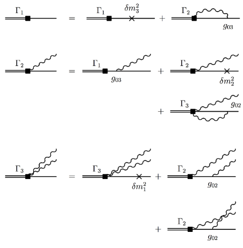
Figure 13: System of equations for the Fock components in a three-body pure scalar model.

The three-body component $\Gamma_{3}$ is expressed through the two-body one, $\Gamma_{2}$, and can be eliminated from the system of equations (99). Since the latter is homogeneous, we can start with a value of $\phi_{1}\equiv\Gamma_{1}/(m^{2}-M^{2})$ equal to one. Dividing Eqs. (99b) and (99c) by $g_{03}$, we get a system of inhomogeneous equations for the (non-normalized) state vector characterized by the Fock components $\bar{\Gamma}_{2,3}\equiv\Gamma_{2,3}/g_{03}$. Excluding $\Gamma_{1}$ and $\Gamma_{3}$ from Eqs. (99) and going over to the limit $M\to m$, we obtain a closed inhomogeneous equation involving the two-body component only:

$$\bar{\Gamma}_{2}^{j}(R_{\perp},x)=1+\frac{g_{02}^{2}\left[\bar{\Sigma}(s^{j}_{1})-\bar{\Sigma}(m^{2})\right]}{m^{2}-s_{1}^{j}}\bar{\Gamma}_{2}^{j}(R_{\perp},x)\\ +\frac{g_{02}^{2}}{16\pi^{3}}\sum_{j^{\prime}}(-1)^{j^{\prime}}\int d^{2}R^{\prime}_{\perp}\int_{0}^{1-x}\frac{dx^{\prime}}{x^{\prime}(1-x^{\prime})}\\ \times\frac{\bar{\Gamma}_{2}^{j^{\prime}}(R^{\prime}_{\perp},x^{\prime})}{(1-x-x^{\prime})(s_{13}^{j^{\prime}}-m^{2})(s_{123}^{jj^{\prime}}-m^{2})},$$ (101)

where

$$s_{1}^{j}=-\frac{R^{2}_{\perp}}{x}+(1-x)m^{2}-\frac{1-x}{x}\mu_{j}^{2}.$$ (102)

The solution $\bar{\Gamma}_{2}^{j}$ of Eq. (101) can be found numerically for given values of $m$ and $g$. It is completely finite in the limit $\mu_{1}\to\infty$. To get the normalized vertex functions, we should calculate the norm $N^{(3)}$ of the state vector. It can be written schematically as

$$N^{(3)}\equiv N_{1}+N_{2}+N_{3}=1+g_{03}^{2}(\bar{N}_{2}+\bar{N}_{3}),$$ (103)

where $\bar{N}_{2,3}$ are the two- and three-body norms written in terms of $\bar{\Gamma}_{2,3}$. The normalized components $\Gamma_{1,2,3}^{R}$ are thus given by

$$\Gamma_{1,2,3}^{R}=\frac{\Gamma_{1,2,3}}{\sqrt{N^{(3)}}}.$$ (104)

We still have to fix the internal BCC $g_{03}$ to calculate the normalized vertex functions. It is found from the requirement that the value of the physical (i.e. taken for $j=0$) two-body vertex function $\Gamma_{2}^{R}$ in the kinematical point ($s^{*}\equiv s_{12}^{j=0}=m^{2},x^{*})$, where $x^{*}$ is a given fixed value of $x$, equals the physical coupling constant:

$$\Gamma_{2}^{R}(s^{*},x^{*})=g.$$ (105)

Let us call $\bar{\Gamma}_{2}^{*}$ the value of $\bar{\Gamma}_{2}^{R}$ in this point. From Eqs. (103)–(105) we get

$$\frac{g_{03}}{\sqrt{1+g_{03}^{2}(\bar{N}_{2}+\bar{N}_{3})}}\bar{\Gamma}_{2}^{*}=g,$$ (106)

which gives

$$g_{03}=\frac{g}{\sqrt{\left[\bar{\Gamma}_{2}^{*}\right]^{2}-g^{2}(\bar{N}_{2}+\bar{N}_{3})}}.$$ (107)

We can see that Eq. (107) is just a generalization of Eq. (100a), since in the absence of the three-body component we have $\bar{\Gamma}_{2}^{*}=1,\bar{N}_{3}=0$, and $\bar{N}_{2}=\bar{I}_{2}$. Using Eqs. (104) and (106), we can represent the normalized vertex function $\Gamma_{2}^{R}$ simply as

$$\Gamma_{2}^{R}=g\frac{\bar{\Gamma}_{2}}{\bar{\Gamma}_{2}^{*}},$$ (108)

which allows to find it directly from the solution of the inhomogeneous equation (101), without calculating explicitly the norm $N^{(3)}$. The latter is just needed to calculate the normalized one-body component $\phi_{1}^{R}=1/\sqrt{N^{(3)}}$.

The substitution of Eq. (107) into Eq. (103) yields

$$N^{(3)}=\frac{\left[\bar{\Gamma}_{2}^{*}\right]^{2}}{\left[\bar{\Gamma}_{2}^{*}\right]^{2}-g^{2}(\bar{N}_{2}+\bar{N}_{3})}.$$ (109)

Finally, substituting the normalized functions $\Gamma_{1}^{R}=\phi_{1}^{R}(m^{2}-M^{2})$ and $\Gamma_{2}^{R}$ into Eq. (99a), we arrive, in the limit $M\to m$, at the following expression for the MC:

$$\delta m_{3}^{2} = -\frac{g^{2}}{\left[\bar{\Gamma}_{2}^{(*)}\right]^{2}-g^{2}(\bar{N}_{2}+\bar{N}_{3})}\sum_{j}\frac{(-1)^{j}}{(2\pi)^{3}}$$ (110)

$$\times\int d^{2}R_{\perp}\int_{0}^{1}\frac{dx}{2x(1-x)}\,\frac{\bar{\Gamma}_{2}^{j}(R_{\perp},x)}{s_{12}^{j}-m^{2}}.\quad\quad$$

The normalized three-body vertex function is found from Eq. (99c), changing $\Gamma_{2}$ to $\Gamma_{2}^{R}$. The norms $\bar{N}_{n}$ are calculated according to

$$\bar{N}_{n} = \frac{2}{(2\pi)^{3(n-1)}(n-1)!}$$ (111)

$$\times\int\prod_{l=1}^{n}\frac{d^{2}R_{l\perp}dx_{l}}{2x_{l}}\left[\frac{\bar{\Gamma}_{n}^{2}}{(s_{n}-m^{2})^{2}}\right]$$

$$\times\delta^{(2)}\left(\sum_{l=1}^{n}{\bf R}_{l\perp}\right)\delta\left(\sum_{l=1}^{n}x_{n}-1\right),$$

where $s_{n}=\sum_{l=1}^{n}(R_{l\perp}^{2}+m_{l}^{2})/x_{l}$ and, in the case of the PV regularization,

$$\bar{\Gamma}_{n}^{2}=\sum_{j_{1}\ldots j_{n-1}}(-1)^{j_{1}+\ldots+j_{n-1}}\bar{\Gamma}_{n}^{j_{1}\ldots j_{n-1}}\bar{\Gamma}_{n}^{j_{1}\ldots j_{n-1}}.$$

In such a way, all unknown parameters are expressed through the solution of the inhomogeneous equation (101).

The application of this strategy to the three-body Fock space truncation in the Yukawa model (one fermion and two scalar bosons) is in progress.

VI Concluding remarks and perspectives

We have presented a systematic strategy to calculate physical observables in CLFD, when Fock space is truncated. This requires to implement an appropriate renormalization scheme in a non-perturbative framework. Within CLFD, we have shown how to fix the counterterms and the BCC’s of the elementary Hamiltonian in a consistent way. As a check of our formalism, we treated the Yukawa model and QED in the two-body approximation, as well as a pure scalar model in the three-body approximation. We were able to recover, for the first time, the standard renormalization of the electromagnetic charge according to the Ward identity, without any perturbative expansion. This shows that no divergences are left uncancelled in the above calculations. Moreover, the first correction to the electron anomalous magnetic moment (the Schwinger correction) is recovered analytically.

Our results have been made possible because of the following three important features of the formalism:

(i) First we can extract the physical part of the two-body vertex function in the point $s=m^{2}$, in order to identify it with the physical coupling constant. This part is explicit in our formalism, since it should be independent of the LF plane orientation determined by the four-vector $\omega$.

(ii) The counterterms and the BCC do depend on the Fock sector, in order to cancel all divergences. We give a well-defined systematic procedure to calculate them.

(iii) We have to distinguish two types of BCC’s: those of the first type are used to calculate the state vector itself, by means of the eigenstate equation, while the BCC’s of the second type are responsible for describing interactions of the constituents with external particles (electromagnetic probes, for example). As we increase the number of Fock sectors, the two BCC’s of different types are expected to converge to the same limit (for finite PV masses).

Our results are very encouraging in the perspective of doing true non-perturbative calculations of bound state systems in a field theoretical framework. In case of success, they may become a real alternative for lattice calculations.

Appendix A Light-front Hamiltonian in the Yukawa model with the Pauli-Villars regularization

We shall find in this section the interaction LF Hamiltonian incorporating PV fields. The methodology is the same as in Ref. [7]. For this reason, we will not give here the detailed algebra with all explicit intermediate results, but outline only the main steps of the procedure.

First, substituting the Lagrangian (10) into Eq. (3) and keeping in mind that now $Y_{i}$ runs through the whole set of the physical and PV fields, we construct the corresponding energy-momentum tensor and then find the four-momentum operator in terms of the Heisenberg fields. In order to have the interaction part of the four-momentum operator in Schrödinger representation, we should find the constraints which connect different field components at the same time and distinguish the independent components. We then express the four-momentum operator through the independent field components only and change after that all the Heisenberg operators by the free ones.

It is convenient to perform calculations in the reference frame where the four-vector $\omega^{\rho}$ has the components $(1,0,0,-1)$ [the four-vector $\omega_{\rho}$ is (1,0,0,1)]. Under this condition the LF ”time” is $x^{+}=x^{0}+x^{3}$, while the ”coordinates” are $x^{-}=x^{0}-x^{3}$ and ${\bf x}^{\perp}=(x^{1},x^{2})$. Analogously, we introduce the plus-, minus-, and transverse components for any four-vector.

The equations of motion for the fermionic fields are

$$(i\gamma^{\nu}\partial_{\nu}-m)\Psi = -(g_{0}\Phi^{\prime}+\delta m)\Psi^{\prime},$$ (112a)

$$(i\gamma^{\nu}\partial_{\nu}-m_{1})\Psi_{PV} = (g_{0}\Phi^{\prime}+\delta m)\Psi^{\prime},$$ (112b)

Splitting the bispinors into the so-called plus- and minus-components (they should not be confused with the plus- and minus-components of four vectors)

$$\Psi=\Psi^{(+)}+\Psi^{(-)},$$ (113)

where

$$\Psi^{(\pm)}=\Lambda^{(\pm)}\Psi,\,\,\,\,\,\,\,\,\Lambda^{(\pm)}=\frac{1}{2}(1\pm\gamma^{0}\gamma^{3})$$ (114)

(and similarly for $\Psi_{PV}$), we can express, by means of Eqs. (112), the minus-components through the plus-ones:

$$\Psi^{(-)} = \frac{\gamma^{0}}{i\partial^{+}}\left[(i{\bf\partial}^{\perp}{\mbox{\boldmath$\gamma$}}^{\perp}+m)\Psi^{(+)}\right.$$ (115a)

$$\left.-(g_{0}\Phi^{\prime}+\delta m){\Psi^{\prime}}^{(+)}\right],$$

$$\Psi^{(-)}_{PV} = \frac{\gamma^{0}}{i\partial^{+}}\left[(i{\bf\partial}^{\perp}{\mbox{\boldmath$\gamma$}}^{\perp}+m_{1})\Psi^{(+)}_{PV}\right.$$ (115b)

$$\left.+(g_{0}\Phi^{\prime}+\delta m){\Psi^{\prime}}^{(+)}\right].$$

The operator $1/(i\partial^{+})$ acting on an arbitrary function $f$ of the coordinate $x$ involves integration over the minus-component of its argument:

$$\frac{1}{i\partial^{+}}f(x^{-})=-\frac{i}{4}\int_{-\infty}^{+\infty}dy^{-}\,\epsilon(x^{-}-y^{-})f(y^{-}),$$ (116)

where $\epsilon$ is the sign function.

Eqs. (115) are constraints, since they do not include the ”time” derivatives $\partial^{-}$ and connect field components at any time. We see that the minus-components of the spinor fields are not independent in the sense that they are expressed through $\Psi^{(+)}$, $\Psi^{(+)}_{PV}$, $\Phi$, and $\Phi_{PV}$. Taking the four latter quantities as independent fields, we can express the four-momentum operator $\hat{P}_{\rho}$ through them. After that, finding this operator in Schrödinger or interaction representation reduces to simple changing the Heisenberg fields $\Psi^{(+)}$, $\Psi^{(+)}_{PV}$, $\Phi$, and $\Phi_{PV}$ by their free counterparts $\psi^{(+)}$, $\psi^{(+)}_{PV}$, $\varphi$, and $\varphi_{PV}$. Splitting, as in Eq. (5), the four-momentum operator into the free and interaction parts, and keeping in mind that $\omega_{+}=(\omega_{0}+\omega_{3})/2=1$, ${\mbox{\boldmath$\omega$}}_{\perp}=-{\mbox{\boldmath$\omega$}}^{\perp}={\bf 0}$, $\omega_{-}=(\omega_{0}-\omega_{3})/2=0$, we obtain from Eq. (6):

$$\hat{P}^{int}_{+}=\frac{1}{2}\int d^{2}x^{\perp}dx^{-}\,H^{int}_{PV}(x).$$ (117)

Calculations performed according to the rules given above yield the formula (11) for the interaction Hamiltonian.

Appendix B CLFD graph technique rules

The graph technique rules for CLFD have already been given in Ref. [6] for the calculation of the $S$-matrix in terms of the operator $-\tilde{H}_{int}$. Since the eigenstate equation (32) is also expressed in terms of the same quantity, these rules are applicable in our case too.

Because of the particular conservation law (29), it is convenient to represent, for the calculation of CLFD diagrams, the momentum $\omega\tau_{n}$ by a separate line, in addition to the ordinary particle lines. This is the so-called spurion line [6]. For practical calculations, one may thus represent the vertex function, as well as any elementary vertex, by the diagrams indicated in Fig. 14. The spurions are shown by the dashed lines.

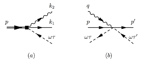
Figure 14: Convenient representation of the vertex function (a) and a typical elementary vertex (b) in terms of the spurion line.

The momentum conservation laws associated to the vertices (a) and (b) in Fig. 14 are, respectively

$$\delta^{(4)}(p+\omega\tau-k_{1}-k_{2})$$

and

$$\delta^{(4)}[p+q-p^{\prime}+\omega(\tau^{\prime}-\tau)].$$

We emphasize that spurions are not considered as true particles. They serve simply for a convenient representation of the departure of intermediate particles from the energy shell.

Appearance of PV fields changes the CLFD graph technique rules, as compared to those listed in Ref. [6]. However, one does not need to re-derive the rules from the very beginning in order to incorporate the changes. Indeed, PV particles can be considered as new fermions and bosons having their own masses and negative norms. Hence, they participate in the construction of CLFD diagrams on equal grounds with physical particles, simply increasing the number of diagrams. The analytical rules to calculate amplitudes of the latter remain almost the same, excepting the expressions for particle propagators. Since physical and PV fields represent two different groups of particles, they can not pair between themselves, i.e. any line in the diagrams relates to either a physical or a PV particle. Pairings within each group are allowed. PV propagators correspond to the PV particle masses and also differ by a sign from the physical ones. In momentum space the propagators are

$$(-1)^{j}\theta(\omega\makebox[2.27626pt]{$\cdot$}p)\delta(p^{2}-\mu_{j}^{2})$$

for bosons and

$$(-1)^{i}({\not\!p}+m_{i})\theta(\omega\makebox[2.27626pt]{$\cdot$}p)\delta(p^{2}-m_{i}^{2})$$

for fermions. The indices $i$ and $j$ describe the particle type: $i=0$ and $j=0$ correspond to physical particles, while $i=1$ and $j=1$ relate to PV ones.

Appendix C Kinematical relations

C.1 One- and two-body kinematics

To calculate the amplitudes of the CLFD diagrams contributing to Eqs. (38) and (39), we need to express the intermediate momenta and their contractions with the external momenta through the variables ${\bf R}_{\perp}$, ${\bf R}^{\prime}_{\perp}$, $x$, and $x^{\prime}$.

The momentum conservation laws in the vertices lead to the following equalities:

$$p_{1i} = p+\omega\tau_{1},$$ (118a)

$$p^{\prime}_{1i^{\prime}} = p+\omega\tau^{\prime}_{1},$$ (118b)

$$k_{1i} = p+\omega\tau_{2}-k_{2j},$$ (118c)

$$k^{\prime}_{1i^{\prime}} = p+\omega\tau^{\prime}_{2}-k^{\prime}_{2j^{\prime}}.$$ (118d)

Squaring the first two of these equations and taking into account that $p^{2}=M^{2}$, $p_{1i}^{2}=m_{i}^{2}$, ${p^{\prime}}_{1i^{\prime}}^{2}=m_{i^{\prime}}^{2}$, and $\omega^{2}=0$, we get

$$\tau_{1}=\frac{m_{i}^{2}-M^{2}}{2\omega\makebox[2.27626pt]{$\cdot$}p},\quad\tau^{\prime}_{1}=\frac{m_{i^{\prime}}^{2}-M^{2}}{2\omega\makebox[2.27626pt]{$\cdot$}p}.$$ (119)

Since, by the definition (37), $\omega\makebox[2.27626pt]{$\cdot$}(k_{2j}-xp)=0$, we have $(k_{2j}-xp)^{2}=-({\bf k}_{2j\perp}-x{\bf p}_{\perp})^{2}=-{R}_{\perp}^{2}$. This allows to represent the scalar product $p\makebox[2.27626pt]{$\cdot$}k_{2j}$ as

$$p\makebox[2.27626pt]{$\cdot$}k_{2j}=\frac{{R}_{\perp}^{2}+M^{2}{x}^{2}+\mu_{j}^{2}}{2x}.$$ (120)

For the scalar product $p\makebox[2.27626pt]{$\cdot$}k^{\prime}_{2j^{\prime}}$ we analogously find

$$p\makebox[2.27626pt]{$\cdot$}k^{\prime}_{2j^{\prime}}=\frac{{R^{\prime}}_{\perp}^{2}+M^{2}{x^{\prime}}^{2}+\mu_{j^{\prime}}^{2}}{2x^{\prime}}.$$ (121)

Squaring Eq. (118c) under the condition ${k}_{1i}^{2}=m_{i}^{2}$, we obtain with the help of Eq. (120):

$$\tau_{2} = \frac{m_{i}^{2}-(p-k_{2j})^{2}}{2\omega\makebox[2.27626pt]{$\cdot$}(p-k_{2j})}$$ (122)

$$= \frac{1}{2\omega\makebox[2.27626pt]{$\cdot$}p}\left[\frac{{R}_{\perp}^{2}+\mu_{j}^{2}}{x}+\frac{{R}_{\perp}^{2}+m_{i}^{2}}{1-x}-M^{2}\right].\quad$$

Analogously,

$$\tau^{\prime}_{2}=\frac{1}{2\omega\makebox[2.27626pt]{$\cdot$}p}\left[\frac{{R^{\prime}}_{\perp}^{2}+\mu_{j^{\prime}}^{2}}{x^{\prime}}+\frac{{R^{\prime}}_{\perp}^{2}+m_{i^{\prime}}^{2}}{1-x^{\prime}}-M^{2}\right].$$ (123)

On the other hand, since $(p+\omega\tau^{\prime}_{2})^{2}=(k^{\prime}_{1i^{\prime}}+k^{\prime}_{2j^{\prime}})^{2}\equiv s_{12}^{i^{\prime}j^{\prime}}$, we have

$$s_{12}^{i^{\prime}j^{\prime}} = M^{2}+2(\omega\makebox[2.27626pt]{$\cdot$}p)\tau^{\prime}_{2}$$ (124)

$$= \frac{{R^{\prime}}_{\perp}^{2}+\mu_{j^{\prime}}^{2}}{x^{\prime}}+\frac{{R^{\prime}}_{\perp}^{2}+m_{i^{\prime}}^{2}}{1-x^{\prime}}.$$

The above equalities are enough to calculate the self-energy (41) and to obtain the system of equations (43) for the scalar components of the vertex functions from the initial system of equations (38).

C.2 Two-body contribution to the three-point Green’s function

To calculate the two-body contribution to the scalar and electromagnetic form factors from the vertices (63b) and (85b), we need to express the contractions of the four-vector $k_{2j}$ with the external momenta $p$ and $p^{\prime}$ through the integration variables ${\bf R}_{\perp}$ and $x$. The contraction $p\makebox[2.27626pt]{$\cdot$}k_{2j}$ is given by Eq. (120). In order to find the scalar product $p^{\prime}\makebox[2.27626pt]{$\cdot$}k_{2j}$, we introduce the four-vector $R^{\prime}\equiv k_{2j}-xp^{\prime}$ and consider its properties. As $\omega\makebox[2.27626pt]{$\cdot$}p=\omega\makebox[2.27626pt]{$\cdot$}p^{\prime}$, we have $\omega\makebox[2.27626pt]{$\cdot$}R^{\prime}=0$ and, hence,

$${R^{\prime}}^{2}=-{R^{\prime}}_{\perp}^{2}=-({\bf k}_{2j\perp}-x{\bf p}_{\perp}-x{\bf q}_{\perp})^{2}$$

$$=({\bf R}_{\perp}-x{\mbox{\boldmath$\Delta$}})^{2}.$$ (125)

On the other hand,

$${R^{\prime}}^{2}=(k_{2j}-xp^{\prime})^{2}=\mu_{j}^{2}-2x(p^{\prime}\makebox[2.27626pt]{$\cdot$}k_{2j})+x^{2}m^{2}.$$ (126)

Comparing the r.-h.s.’s of Eqs. (125) and (126), we finally get

$$p^{\prime}\makebox[2.27626pt]{$\cdot$}k_{2j}=\frac{({\bf R}_{\perp}-x{\mbox{\boldmath$\Delta$}})^{2}+\mu_{j}^{2}+x^{2}m^{2}}{2x}.$$ (127)

C.3 Three-body kinematics

To cast the equations for the vertex functions in the three-body approximation to the form (99), we should define due kinematical variables. For this purpose, we consider a set of three four-vectors

$$R_{n}=k_{n}-x_{n}p,$$ (128)

where $n=1,\,2,\,3$ and $x_{n}=(\omega\makebox[2.27626pt]{$\cdot$}k_{n})/(\omega\makebox[2.27626pt]{$\cdot$}p)$. The four-vectors $k_{n}$ are just the four-momenta of the constituents. For shortness, we do not pay attention to the particle type (physical or PV one). The momentum conservation law reads

$$\sum_{n}k_{n}=p+\omega\tau_{3},$$ (129)

where $\omega\tau_{3}$ is the spurion momentum in the three-body state. Contracting both sides of Eq. (129) with $\omega$, we have

$$\sum_{n}x_{n}=1.$$ (130)

The substitution of $k_{n}=R_{n}+x_{n}p$ into Eq. (129) gives

$$\sum_{n}R_{n}=\omega\tau_{3}$$ (131)

and, hence,

$$\sum_{n}{\bf R}_{n\perp}={\bf 0}.$$ (132)

Because of Eqs. (130) and (132), only two of the three ${\bf R}_{\perp}$’s and two of the three $x$’s are independent. We will choose as independent variables those for the bosons, while the ”nucleon” variables are expressed through them as

$${\bf R}_{1\perp}=-({\bf R}_{2\perp}+{\bf R}_{3\perp}),\quad x_{1}=1-x_{2}-x_{3}.$$ (133)

We also need to know the contractions of the four-momenta $p$ and $k_{n}$ among themselves. Since for all $n$ we have $\omega\makebox[2.27626pt]{$\cdot$}R_{n}=0$, $R_{n}^{2}=-R_{n\perp}^{2}$, then, in full analogy with the derivation of Eq. (120),

$$p\makebox[2.27626pt]{$\cdot$}k_{n}=\frac{{R}_{n\perp}^{2}+M^{2}{x}_{n}^{2}+m_{n}^{2}}{2x_{n}},$$ (134)

where $m_{n}$ is the mass related to the particle $n$. From the condition $\omega\makebox[2.27626pt]{$\cdot$}R_{n}=0$ follows

$$R_{n_{1}}\makebox[2.27626pt]{$\cdot$}R_{n_{2}} = -{\bf R}_{n_{1}\perp}{\bf R}_{n_{2}\perp}$$ (135)

$$= (k_{n_{1}}-x_{n_{1}}p)\makebox[2.27626pt]{$\cdot$}(k_{n_{2}}-x_{n_{2}}p),$$

which finally yields

$$k_{n_{1}}\makebox[2.27626pt]{$\cdot$}k_{n_{2}} = \frac{x_{n_{2}}}{2x_{n_{1}}}({R}_{n_{1}\perp}^{2}+m_{n_{1}}^{2})$$

$$+\frac{x_{n_{1}}}{2x_{n_{2}}}({R}_{n_{2}\perp}^{2}+m_{n_{2}}^{2})-{\bf R}_{n_{1}\perp}{\bf R}_{n_{2}\perp}.$$

It is also convenient to define the invariant energy squared of the three-body state:

$$s_{123}\equiv\left(\sum_{n}k_{n}\right)^{2}=\sum_{n}\frac{{R}_{n\perp}^{2}+m_{n}^{2}}{x_{n}}.$$ (137)

Omitting the subscript 2 at ${\bf R}_{2\perp}$ and $x_{2}$, and changing ${\bf R}_{3\perp}\to{\bf R}^{\prime}_{\perp}$, $x_{3}\to x^{\prime}$ everywhere in the above formulas, we transform the equations for the vertex functions, obtained from the diagrams of Fig. 13, to those given by Eqs. (99).

References

- [1] P.A.M. Dirac, Rev. Mod. Phys. 21, 392 (1949).
-
[2]
T. Heinzl, S. Krusche and E. Werner, Phys. Lett. 256, 55 (1991) ;
T. Heinzl, S. Krusche, S. Simbürger, E. Werner, Z. Phys., C56, 415 (1992). -
[3]
P. Grangé, P. Ullrich and E. Werner, Phys. Rev. D57, 4981 (1998);
S. Salmons, P. Grangé and E. Werner, Phys. Rev. D65, 125014 (2002) . - [4] D.S. Hwang and V.A. Karmanov, Nucl. Phys. B696, 413 (2004).
- [5] V.A. Karmanov, Zh. Eksp. Teor. Fiz. 71, 399 (1976) [trans.:JETP 44, 210 (1976)].
- [6] J. Carbonell, B. Desplanques, V.A. Karmanov and J.-F. Mathiot, Phys. Rep. 300, 215 (1998).
- [7] V.A. Karmanov, J.-F. Mathiot and A.V. Smirnov, Phys. Rev. D69, 045009 (2004).
- [8] V.A. Karmanov, J.-F. Mathiot and A.V. Smirnov, Phys. Rev. D75, 045012 (2007).
-
[9]
N.E. Ligterink and B.L.G. Bakker, Phys. Rev. D 52, 5917,
5954 (1995);
N.C.J. Schoonderwoerd and B.L.G. Bakker, Phys. Rev. D 58, 025013 (1998);
B.L.G. Bakker, M.A. DeWitt, Ch.-R. Ji and Yu. Mishchenko, Phys. Rev. D 72, 076005 (2005). - [10] S. Glazek et al., Phys. Rev. D47, 1599 (1993).
- [11] S.J. Brodsky, J. Hiller and G. McCartor, Phys. Rev. D59, 016006 (1999).
- [12] S.J. Brodsky, J. Hiller and G. McCartor, Phys. Rev. D64, 114023 (2001).
- [13] S.J. Brodsky et al., Nucl. Phys.B703, 333 (2004).
- [14] S.J. Brodsky, J. Hiller and G. McCartor, Ann. Phys. 305, 266 (2003).
- [15] S.J. Brodsky, J. Hiller and G. McCartor, Ann. Phys. 321, 1240 (2006).
- [16] R. Perry, A. Harindranath and K. Wilson, Phys. Rev. Lett. 65, 2959 (1990).
- [17] J.-F. Mathiot, V.A. Karmanov and A.V. Smirnov, Few-Body Systems 36, 173 (2005).
- [18] M.E. Peskin, D.V. Schroeder, ”An Introduction to Quantum Field Theory”, Perseus Books, (1995)
- [19] V.A. Karmanov, Zh. Eksp. Teor. Fiz. 83, 3 (1982) [trans.:JETP 56, 1 (1982)].
- [20] D. Bernard, Th. Cousin, V.A. Karmanov and J.-F. Mathiot, Phys. Rev. D65, 025016 (2001).
- [21] V.A. Karmanov and J.-F. Mathiot, Nucl. Phys. A602, 388 (1996).
- [22] J. Schwinger (Ed.), Quantum Electrodynamics, selected papers, Dover New York (1958).