On the birth-and-assassination process, with an application to scotching a rumor in a network

Abstract

We give new formulas on the total number of born particles in the stable birth-and-assassination process, and prove that it has a heavy-tailed distribution. We also establish that this process is a scaling limit of a process of rumor scotching in a network, and is related to a predator-prey dynamics.

Keywords: branching process, heavy tail phenomena, SIR epidemics.

MSC-class: 60J80.

1 Introduction

Birth-and-assassination process

The birth-and-assassination process was introduced by Aldous and Krebs [2], it is a variant of the branching process. The original motivation of the authors was then to analyze a scaling limit of a queueing process with blocking which appeared in database processing, see Tsitsiklis, Papadimitriou and Humblet [14]. In this paper, we show that the birth-and-assassination process exhibits some heavy-tailed distribution. For general references on heavy-tail distribution in queueing processes, see for example Mitzenmacher [9] or Resnick [12]. In this paper, we will not discuss this application. Instead, we will show that the birth-and-assassination process is also the scaling limit of a rumor spreading model which is motivated by network epidemics and dynamic data dissemination (see for example, [10], [4], [11]).

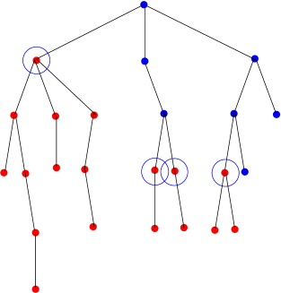
Figure 1: Illustration of the birth-and-assassination process, living particles are in red, dead particles in blue, particles at risk are encircled.

We now reproduce the formal definition of the birth-and-assassination process from [2]. Let $\mathbb{N}^{f}=\cup_{k=0}^{\infty}\mathbb{N}^{k}$ be the set of finite k-tuples of positive integers (with $N^{0}=\emptyset$). Let $\{\Phi_{\bf n}\},{\bf n}\in\mathbb{N}^{f}$, be a family of independent Poisson processes with common arrival rate $\lambda$. Let $\{K_{\bf n}\},{\bf n}\in\mathbb{N}^{f}$, be a family of independent, identically distributed (iid), strictly positive random variables. Suppose the families $\{\Phi_{\bf n}\}$ and $\{K_{\bf n}\}$ are independent. The particle system starts at time $0$ with only the ancestor particle, indexed by $\emptyset$. This particle produces offspring at the arrival times of $\Phi_{\emptyset}$, which enter the system with indices $(1)$, $(2)$, $\cdots$ according to their birth order. Each new particle ${\bf n}$ entering the system immediately begins producing offspring at the arrival times of $\{\Phi_{\bf n}\}$, the offspring of ${\bf n}$ are indexed $({\bf n},1)$, $({\bf n},2)$, $\cdots$ also according to birth order. The ancestor particle is at risk at time $0$. It continues to produce offspring until time $D_{\emptyset}=K_{\emptyset}$, when it dies. Let $k>0$ and let ${\bf n}=(n_{1},\cdots,n_{k-1},n_{k})$, ${\bf n}^{\prime}=(n_{1},...,n_{k-1})$. When a particle ${\bf n}^{\prime}$ dies (at time $D_{{\bf n}^{\prime}}$), ${\bf n}$ then becomes at risk; it continues to produce offspring until time $D_{\bf n}=D_{{\bf n}^{\prime}}+K_{\bf n}$, when it dies. We will say that the birth-and-assassination process is stable if with probability $1$ there exists some time $t<\infty$ with no living particle. The process is unstable if it is not stable. Aldous and Krebs [2] proved the following:

Theorem 1 (Aldous and Krebs)

Consider a birth-and-assassination process with offspring rate $\lambda$ whose killing distribution has moment generating function $\phi$. Suppose $\phi$ is finite in some neighborhood of $0$. If $\min_{u>0}\lambda u^{-1}\phi(u)<1$ then the process is stable. If $\min_{u>0}\lambda u^{-1}\phi(u)>1$ then the process is unstable.

The birth-and-assassination process is a variant the classical branching process. Indeed, if instead the particle ${\bf n}$ is at risk not when its parent dies but when the particle ${\bf n}$ was born, then we obtain a well-studied type of branching process, refer to Athreya and Ney [5]. The populations in successive generations behave as the simple Galton-Walton branching process with mean offspring equal to $\lambda{\mathrm{E}}K_{\emptyset}$, and so the process is stable if this mean is less than $1$. The birth-and-assassination process is a variation in which the ’clock’ which counts down the time until a particle’s death does not start ticking until the particle’s parent dies.

In this paper, we will pay attention to the special case where the killing distribution is an exponential distribution with intensity $\mu$. By a straightforward scaling argument, a birth-and-assassination process with intensities $(\lambda,\mu)$ and a birth-and-assassination process with intensities $(\lambda\mu^{-1},1)$ where the time is accelerated by a factor $\mu$ have the same distribution. Therefore, without loss of generality, from now on, we will consider ${\cal B}$, a birth-and-assassination process with intensities $(\lambda,1)$. As a corollary of Theorem 1, we get

Corollary 1 (Aldous and Krebs)

If $0<\lambda<1/4$, the process ${\cal B}$ is stable. If $\lambda>1/4$, the process ${\cal B}$ is unstable.

In the first part of this paper, we study the behavior of the process ${\cal B}$ in the stable regime, especially as $\lambda$ get close to $1/4$. We introduce a family of probability measures $\{{\mathrm{P}}_{\lambda}\},\lambda>0,$ on our underlying probability space such that under ${\mathrm{P}}_{\lambda}$, ${\cal B}$ is a birth-and-assassination process with intensities $(\lambda,1)$. Let $\lambda\in(0,1/4)$, we define $N$ as the total number of born particles in ${\cal B}$ (including the ancestor particle) and

$$\gamma(\lambda)=\sup\left\{u\geq 0:{\mathrm{E}}_{\lambda}N^{u}<\infty\right\}.$$

In particular, if $0<\gamma(\lambda)<\infty$, from Markov Inequality, for all $0<\epsilon<\gamma(\lambda)$, there exists a constant $C\geq 1$ such that for all $t\geq 1$,

$${\mathrm{P}}_{\lambda}(N>t)\leq Ct^{-\gamma(\lambda)+\epsilon}.$$

The number $\gamma$ may thus be interpreted as a power tail exponent. There is a simple expression for $\gamma$.

Theorem 2

For all $\lambda\in(0,1/4)$,

$$\gamma(\lambda)=\frac{1+\sqrt{1-4\lambda}}{1-\sqrt{1-4\lambda}}.$$

This result contrasts with the behavior of the classical branching process, where for all $\lambda<1$: there exists a constant $c>0$ such that ${\mathrm{E}}_{\lambda}\exp(cN)<\infty$. This heavy tail behavior of the birth-and-assassination process is thus a striking feature of this process. Near criticality, as $\lambda\uparrow 1/4$, we get $\gamma(\lambda)\sim 1$, whereas as $\lambda\downarrow 0$, we find $\gamma(\lambda)\sim(2\lambda)^{-1}$. By recursion, we will also compute the moments of $N$.

Theorem 3

• For all $p\geq 2$, ${\mathrm{E}}_{\lambda}N^{p}<\infty$ if and only if $\lambda\in(0,p(p+1)^{-2})$.

• If $\lambda\in(0,1/4]$,

  $${\mathrm{E}}_{\lambda}N=\frac{2}{1+\sqrt{1-4\lambda}}.$$ (1)

• If $\lambda\in(0,2/9)$,

  $${\mathrm{E}}_{\lambda}N^{2}=\frac{2}{3\sqrt{1-4\lambda}-1}.$$ (2)

Theorem 3(i) is consistent with Theorem 2: $\lambda\in(0,p(p+1)^{-2})$ is equivalent to $p\in[1,(1+\sqrt{1-4\lambda})(1-\sqrt{1-4\lambda})^{-1})$ . Theorem 3(ii) implies a surprising discontinuity of the function $\lambda\mapsto{\mathrm{E}}_{\lambda}N$ at the critical intensity $\lambda=1/4$: $\lim_{\lambda\uparrow 1/4}{\mathrm{E}}_{\lambda}N=2$. Again, this discontinuity contrasts with what happens in a standard Galton-Watson process near criticality, where for $0<\lambda<1$, ${\mathrm{E}}_{\lambda}N=(1-\lambda)^{-1}$. We will prove also that this discontinuity is specific to $\lambda=1/4$ and for all $p\geq 2$, $\lim_{\lambda\uparrow p(p+1)^{-2}}{\mathrm{E}}_{\lambda}[N^{p}]=\infty$. We will explain a method to compute all integers moments of $N$ by recursion. The third moment has already a complicated expression (see §2.5.1). From Theorem 3(ii), we may fill the gap in Corollary 1.

Corollary 2

If $\lambda=1/4$, the process ${\cal B}$ is stable.

In Section 2, we will prove Theorems 2 and 3 by exhibiting a Recursive Distributional Equation (RDE) for a random variable related to $N$. Unfortunately, our method does not give much insights on the heavy-tail phenomena involved in the birth-and-assassination process.

Rumor scotching process

We now define the rumor scotching process on a graph. It is a nonstandard SIR dynamics (see for example [10] or [4] for some background). This process represents the dynamics of a rumor/epidemic spreading on the vertices of a graph along its edges. A vertex may be unaware of the rumor/susceptible (S), aware of the rumor and spreading it as true/infected (I), or aware of the rumor and trying to scotch it/recovered (R).

More formally, we fix a connected graph $G=(V,E)$, and let ${\cal P}_{V}$ denote the set of subsets of $V$ and ${\cal X}=({\cal P}_{V}\times\{S,I,R\})^{V}$. The spread of the rumor is described by a Markov process on ${\cal X}$. For $X=(X_{v})_{v\in V}\in{\cal X}$, with $X_{v}=(A_{v},s_{v})$, $A_{v}$ is interpreted as the set of neighbors of $v$ which can change the opinion of $v$ on the veracity of the rumor. If $(uv)\in E$, we define the operations $E_{uv}$ and $E_{v}$ on ${\cal X}$ by $(X+E_{uv})_{w}=(X-E_{v})_{w}=X_{w}$, if $w\neq v$ and $(X+E_{uv})_{v}=(A_{v}\cup\{u\},I)$, $(X-E_{v})_{v}=(\emptyset,R)$. Let $\lambda>0$ be a fixed intensity, the rumor scotching process is the Markov process with generator:

$$K(X,X+E_{uv}) = \lambda{\bf 1}(s_{u}=I){\bf 1}((u,v)\in E){\bf 1}(s_{v}\neq R),$$

$$K(X,X-E_{v}) = {\bf 1}(s_{v}=I)\sum_{u\in A_{v}}{\bf 1}(s_{u}=R),$$

and all other transitions have rate $0$. Typically, at time $0$, there is non-empty finite set of $I$-vertices and there is a vertex $v$ such that $A_{v}$ contains a $R$-vertex. The absorbing states of this process are the states without $I$-vertices. The case when at time $0$, $A_{v}$ is the set to all neighbors of $v$ is interesting in its own (there, $A_{v}$ does not evolve before $s_{v}=R$).

If $G$ is the infinite $k$-ary tree this process has been analyzed by Kordzakhia [7] and it was defined there as the chase-escape model. It is thought as a predator-prey dynamics: each vertex may be unoccupied (S), occupied by a prey (I) or occupied by a predator (R). The preys spread on unoccupied vertices and predators spread on vertices occupied by preys. If $G$ is the ${\mathbb{Z}}^{d}$-lattice and if there is no $R$-vertices, the process is the original Richardson’s model [13]. With $R$-vertices, this process is a variant of the two-species Richardson model with prey and predators, see for example Häggström and Pemantle [6], Kordzakhia and Lalley [8]. Nothing is apparently known on this process.

In Section 3, we show that the birth-and-assassination process is the scaling limit, as $n$ goes to infinity, of the rumor scotching process when $G$ is the complete graph over $n$ vertices and the intensity is $\lambda/n$ (Theorem 4).

2 Integral equations for the birth-and-assassination process

2.1 Proof of Theorem 3 for the first moment

In this paragraph, we prove Theorem 3(ii). Let $X(t)\in[0,+\infty]$ be the total number of born particles in the process ${\cal B}$ given that the root cannot die before time $t$, and $Y(t)$ be the total number of born particles given that the root dies at time $t$. By definition, if $D$ is an exponential variable with mean $1$ independent of $Y$, then $N\stackrel{{\scriptstyle d}}{{=}}X(0)\stackrel{{\scriptstyle d}}{{=}}Y(D)$, where the symbol $\stackrel{{\scriptstyle d}}{{=}}$ stands for distributional equality. We notice also that the memoryless property of the exponential variable implies $X(t)\stackrel{{\scriptstyle d}}{{=}}Y(t+D)$. The recursive structure of the birth-and-assassination process leads to the following equality in distribution

$$Y(t)\stackrel{{\scriptstyle d}}{{=}}1+\sum_{i:\xi_{i}\leq t}X_{i}(t-\xi_{i})\stackrel{{\scriptstyle d}}{{=}}1+\sum_{i:\xi_{i}\leq t}X_{i}(\xi_{i}),$$

where $\Phi=\{\xi_{i}\}_{i\in\mathbb{N}}$ is a Poisson point process of intensity $\lambda$ and $(X_{i}),i\in\mathbb{N},$ are independent copies of $X$. Note that since all variables are non-negative, there is no issue with the case $Y(t)=+\infty$. We obtain the following RDE for the random function $Y$:

$$Y(t)\stackrel{{\scriptstyle d}}{{=}}1+\sum_{i:\xi_{i}\leq t}Y_{i}(\xi_{i}+D_{i}),$$ (3)

where $Y_{i},$ and $D_{i}$ are independent copies of $Y$ and $D$ respectively. This last RDE is the cornerstone of this work.

Assuming that ${\mathrm{E}}_{\lambda}N<\infty$ we first prove that necessarily $\lambda\in(0,1/4)$. For convenience, we often drop the parameter $\lambda$ in ${\mathrm{E}}_{\lambda}$ and other objects depending on $\lambda$. From Fubini’s theorem, ${\mathrm{E}}X(0)={\mathrm{E}}N=\int_{0}^{\infty}{\mathrm{E}}Y(t)e^{-t}dt$ and therefore ${\mathrm{E}}Y(t)<\infty$ for almost all $t\geq 0$. Note however that since $t\mapsto Y(t)$ is monotone for the stochastic domination, it implies that ${\mathrm{E}}Y(t)<\infty$ for all $t>0$. The same argument gives the next lemma.

Lemma 1

Let $t>0$ and $u>0$, if ${\mathrm{E}}[N^{u}]<\infty$ then ${\mathrm{E}}[Y(t)^{u}]<\infty$.

Now, taking expectation in (3), we get

$${\mathrm{E}}Y(t) = 1+\lambda\int_{0}^{t}\int_{0}^{\infty}{\mathrm{E}}Y(x+s)e^{-s}dsdx.$$

Let $f_{1}(t)={\mathrm{E}}Y(t)$, it satisfies the integral equation, for all $t\geq 0$,

$$f_{1}(t)=1+\lambda\int_{0}^{t}e^{x}\int_{x}^{\infty}f_{1}(s)e^{-s}dsdx.$$ (4)

Taking the derivative once and multiplying by $e^{-t}$, we get: $f^{\prime}_{1}(t)e^{-t}=\lambda\int_{t}^{\infty}f_{1}(s)e^{-s}ds.$ Then, taking the derivative a second time and multiplying by $e^{t}$: $f_{1}^{\prime\prime}(t)-f_{1}^{\prime}(t)=-\lambda f_{1}(t).$ So, finally, $f_{1}$ solves a linear ordinary differential equation of the second order

$$x^{\prime\prime}-x^{\prime}+\lambda x=0,$$ (5)

with initial condition $x(0)=1$. If $\lambda>1/4$ the solutions of (5) are

$$x(t)=e^{t/2}(\cos(t\sqrt{4\lambda-1})+a\sin(t\sqrt{4\lambda-1})),$$

for some constant $a$. Since $f_{1}(t)$ is necessarily positive, this leads to a contradiction and ${\mathrm{E}}N=\infty$. Assume now that $0<\lambda<1/4$ and let

$$\Delta=\sqrt{1-4\lambda}\;\hbox{ , }\quad\alpha=\frac{1-\Delta}{2}\quad\hbox{ and }\quad\beta=\frac{1+\Delta}{2}.$$ (6)

$(\alpha,\beta)$ are the roots of the polynomial $X^{2}-X+\lambda=0$. The solutions of (5) are

$$x_{a}(t)=(1-a)e^{\alpha t}+ae^{\beta t}$$

for some constant $a$. Whereas, for $\lambda=1/4$, $\alpha=1/2$ and the solutions of (5) are

$$x_{a}(t)=(at+1)e^{t/2}.$$

For $0<\lambda\leq 1/4$, we check easily that the functions $x_{a}$ with $a\geq 0$ are the nonnegative solutions of the integral equation (4).

It remains to prove that if $0<\lambda\leq 1/4$ then ${\mathrm{E}}N<\infty$ and $f_{1}(t)=e^{\alpha t}.$ Indeed, then ${\mathrm{E}}N=\int_{0}^{\infty}f_{1}(t)e^{-t}dt=(1-\alpha)^{-1}$ as stated in Theorem 3(ii). To this end, define $f_{1}^{(n)}(t)={\mathrm{E}}\min(Y(t),n)$, from (3),

$$\min(Y(t),n)\leq_{st}1+\sum_{i:\xi_{i}\leq t}\min(Y_{i}(\xi_{i}+D_{i}),n).$$

Taking expectation, we obtain, for all $t\geq 0$,

$$f_{1}^{(n)}(t)\leq 1+\lambda\int_{0}^{t}e^{x}\int_{x}^{\infty}f_{1}^{(n)}(s)e^{-s}dsdx.$$ (7)

We now state a lemma which will be used multiple times in this paper. We define

$$\overline{\gamma}(\lambda)=(1+\Delta)/(1-\Delta)=\beta/\alpha.$$ (8)

Let $1<u<\overline{\gamma}$ (or equivalently $\lambda<u(u+1)^{-2}$), we define ${\cal H}_{u}$, the set of measurable functions $h:[0,\infty)\to[0,\infty)$ such that $h$ is non-decreasing and $\sup_{t\geq 0}h(t)e^{-u\alpha t}<\infty$. Let $C>0$, we define the mapping from ${\cal H}_{u}$ to ${\cal H}_{u}$,

$$\Psi:h\mapsto Ce^{u\alpha t}+\lambda\int_{0}^{t}e^{x}\int_{x}^{\infty}h(s)e^{-s}dsdx.$$

In order to check that $\Psi$ is indeed a mapping from ${\cal H}_{u}$ to ${\cal H}_{u}$, we use the fact that if $1<u<\overline{\gamma}$, then $u\alpha<1$. Note also that if $1<u<\overline{\gamma}$, then $u\alpha-\lambda-u^{2}\alpha^{2}>0$. If $\lambda=1/4$, we also define the mapping from ${\cal H}_{1}$ to ${\cal H}_{1}$,

$$\Phi:h\mapsto 1+\frac{1}{4}\int_{0}^{t}e^{x}\int_{x}^{\infty}h(s)e^{-s}dsdx.$$

(recall that for $\lambda=1/4$, $\alpha=1/2$).

Lemma 2

1. Let $1<u<\overline{\gamma}$ and $f\in{\cal H}_{u}$ such that $f\leq\Psi(f)$. Then for all $t\geq 0$,

   $$f(t)\leq C\frac{u\alpha(1-u\alpha)}{u\alpha-\lambda-u^{2}\alpha^{2}}e^{u\alpha t}-C\frac{\lambda}{u\alpha-\lambda-u^{2}\alpha^{2}}e^{\alpha t}.$$

2. If $\lambda=1/4$ and $f\in{\cal H}_{1}$ is such that $f\leq\Phi(f)$, then for all $t\geq 0$,

   $$f(t)\leq e^{t/2}.$$

Before proving Lemma 2, we conclude the proof of Theorem 3$(ii)$. For $0<\lambda<1/4$, from (7), we may apply Lemma 2(i) applied to $1<u<\beta/\alpha$, $C=1$. We get that

$$f_{1}^{(n)}(t)\leq C_{u}e^{\alpha ut}$$

for some $C_{u}>0$. The monotone convergence theorem implies that $f_{1}(t)=\lim_{n\to\infty}f_{1}^{(n)}(t)$ exists and is bounded by $C_{u}e^{\alpha ut}$. Therefore $f_{1}$ solves the integral equation (4) and is equal to $x_{a}$ for some $a\geq 0$. From what precedes, we get $x_{a}(t)\leq C_{u}e^{\alpha ut}$, however, since $\alpha u<\beta$, the only possibility is $a=0$ and $f_{1}(t)=e^{\alpha t}$.

Similarly, if $\lambda=1/4$, from Lemma 2$(ii)$, $f_{1}(t)\leq e^{t/2}.$ This proves that $f_{1}$ is finite, and we thus have $f_{1}=x_{a}$ for some $a\geq 0$. Again, the only possibility is $a=0$ since $x_{a}(t)\leq e^{t/2}$ implies $a=0$.

Proof of Lemma 2. $(i)$. The fixed points of the mapping $\Psi$ are the functions $h_{a,b}$ such that

$$h_{a,b}(t)=ae^{\alpha t}+be^{\beta t}+C\frac{u\alpha(1-u\alpha)}{u\alpha-\lambda-u^{2}\alpha^{2}}e^{u\alpha t},$$

with $a+b+C\frac{u\alpha(1-u\alpha)}{u\alpha-\lambda-u^{2}\alpha^{2}}=C$. The only fixed point in ${\cal H}_{u}$ is $h_{*}:=h_{a_{*},0}$ with $a_{*}=-C\lambda/(u\alpha-\lambda-u^{2}\alpha^{2})$. Let ${\cal C}_{u}$ denote the set of continuous functions in ${\cal H}_{u}$, note that $\Psi$ is also a mapping from ${\cal C}_{u}$ to ${\cal C}_{u}$. Now let $g_{0}\in{\cal C}_{u}$ and for $k\geq 1$, $g_{k}=\Psi(g_{k-1})$. We first prove that for all $t\geq 0$ , $\lim_{k}g_{k}(t)=h_{*}(t)$. If $1<u<\overline{\gamma}$ then $u\alpha(1-u\alpha)>\lambda$ and $\frac{u\alpha(1-u\alpha)}{u\alpha-\lambda-u^{2}\alpha^{2}}$ is positive. We deduce easily that if $g_{0}(t)\leq Le^{u\alpha t}$ then $g_{1}(t)=\Psi(g)(t)\leq Ce^{u\alpha t}+\frac{L\lambda}{u\alpha(1-u\alpha)}(e^{u\alpha t}-1)\leq L_{1}e^{u\alpha t}$, with $L_{1}=(C+\frac{L\lambda}{u\alpha(1-u\alpha)})$. By recursion, we obtain that $\limsup_{k}g_{k}(t)\leq L_{\infty}e^{u\alpha t}$, with $L_{\infty}=Cu\alpha(1-u\alpha)/(u\alpha-\lambda-u^{2}\alpha^{2})<\infty$. From Arzela-Ascoli’s theorem, $(g_{k})_{k\in\mathbb{N}}$ is relatively compact in ${\cal C}_{u}$ and any accumulation point converges to $h_{*}$ (since $h_{*}$ is the only fixed point of $\Psi$ in ${\cal C}_{u}$).

Now since $f\in{\cal H}_{u}$, there exists a constant $L>0$ such that for all $t\geq 0$, $f(t)\leq g_{0}(t):=Le^{u\alpha t}$. The monotonicity of the mapping $\Psi$ implies that $\Psi(f)\leq\Psi(g_{0})=g_{1}$. By assumption, $f\leq\Psi(f)$ thus by recursion $f\leq\lim_{n}g_{n}=h_{*}$.

$(ii)$. The function $x_{0}(t)=e^{t/2}$ is the only fixed point of $\Phi$ in ${\cal H}_{1}$. Moreover, if $g(t)\leq Ce^{t/2}$ then we also have $\Phi(g)(t)\leq Ce^{t/2}$. Then, if $g$ is continuous, arguing as above, from Arzela-Ascoli’s theorem, $(\Phi^{k}(g))_{k\in\mathbb{N}}$ converges to $x_{0}$. We conclude as in (i). $\Box$

2.2 Proof of Theorem 3(i)

We define $f_{p}(t)={\mathrm{E}}_{\lambda}[Y(t)^{p}]$. As above, we often drop the parameter $\lambda$ in ${\mathrm{E}}_{\lambda}$ and other objects depending on $\lambda$.

Lemma 3

Let $p\geq 2$, there exists a polynomial $Q_{p}$ with degree $p$ such that for all $t>0$,

• If $\lambda\in(0,p(p+1)^{-2})$, then $f_{p}(t)=Q_{p}(e^{\alpha t})$.

• If $\lambda\geq p(p+1)^{-2}$, then $f_{p}(t)=\infty$,

Note that if such polynomial $Q_{p}$ exists then $Q_{p}(x)\geq 1$ for all $x\geq 1$. Note also that $\lambda\in(0,p(p+1)^{-2})$ implies that $p<\overline{\gamma}=\beta/\alpha$ (where $\overline{\gamma}$ was defined by (8)), and thus $p\alpha<\beta<1$. Hence Lemma 3 implies Theorem 3(i) since ${\mathrm{E}}[N^{p}]=\int f_{p}(t)e^{-t}dt$.

Let $\kappa_{p}(X)$ denote the $p^{th}$ cumulant of a random variable $X$ whose moment generating function is defined in a neighborhood of $0$: $\ln{\mathrm{E}}e^{\theta X}=\sum_{p\geq 0}\kappa_{p}(X)\theta^{p}/p!$. In particular $\kappa_{0}(X)=0$, $\kappa_{1}(X)={\mathrm{E}}X$ and $\kappa_{2}(X)={\mathrm{Var}}X$. Using the exponential formula

$${\mathrm{E}}\exp{\sum_{\xi_{i}\in\Phi}h(\xi_{i},Z_{i})}=\exp(\lambda\int_{0}^{\infty}({\mathrm{E}}e^{h(x,Z)}-1)dx),$$ (9)

valid for all non-negative function $h$ and iid variables $(Z_{i}),i\in\mathbb{N}$, independent of $\Phi=\{\xi_{i}\}_{i\in\mathbb{N}}$ a Poisson point process of intensity $\lambda$, we obtain that for all $p\geq 1$,

$$\kappa_{p}\left(\sum_{i:\xi_{i}\leq t}h(\xi_{i},Z_{i})\right)=\lambda\int_{0}^{t}{\mathrm{E}}h^{p}(x,Z)dx.$$ (10)

Due to this last formula, it will be easier to deal with the cumulant $g_{p}(t)=\kappa_{p}(Y(t))$. By recursion, we will prove the next lemma which implies Lemma 3.

Lemma 4

Let $p\geq 2$, there exists a polynomial $R_{p}$ with degree $p$, positive on $[1,\infty)$ such that, for all $t>0$,

• If $\lambda\in(0,p(p+1)^{-2})$, then $f_{p}(t)<\infty$ and $g_{p}(t)=R_{p}(e^{\alpha t})$.

• If $\lambda\geq p(p+1)^{-2}$, then $f_{p}(t)=\infty$,

Proof of Lemma 4. In §2.1, we have computed $f_{p}$ for $p=1$ and found $R_{1}(x)=x$. Let $p\geq 2$ and assume now that the statement of the Lemma 4 holds for $q=1,\cdots,p-1$. We assume first that $f_{p}(t)<\infty$, we shall prove that necessarily $\lambda\in(0,p(p+1)^{-2})$ and $g_{p}(t)=R_{p}(e^{\alpha t})$. Without loss of generality we assume that $0<\lambda<1/4$. From Fubini’s theorem, using the linearity of cumulants in (3) and (10), we get

$$g_{p}(t) = \lambda\int_{0}^{t}\int_{0}^{\infty}{\mathrm{E}}[Y(x+s)^{p}]e^{-s}dsdx$$ (11)

$$= \lambda\int_{0}^{t}e^{x}\int_{x}^{\infty}f_{p}(s)e^{-s}dsdx,$$

(note that Fubini’s Theorem implies the existence of $f_{p}(s)$ for all $s>0$). From Jensen inequality $f_{p}(t)\geq g_{1}(t)^{p}=e^{p\alpha t}$ and the integral $\int_{x}^{\infty}e^{p\alpha s}e^{-s}dsdx$ is finite if and only if $p\alpha<1$. We may thus assume that $p\alpha<1$. We now recall the identity: ${\mathrm{E}}X^{p}=\sum_{\pi}\prod_{I\in\pi}\kappa_{|I|}(X)$, where the sum is over all set partitions of $\{1,\cdots,p\}$, $I\in\pi$ means $I$ is one of the subsets into which the set is partitioned, and $|I|$ is the cardinal of $I$. This formula implies that ${\mathrm{E}}X^{p}=\kappa_{p}(X)+\Sigma_{p-1}(\kappa_{1}(X),\cdots,\kappa_{p-1}(X))$, where $\Sigma_{p-1}(x_{1},\cdots,x_{p-1})$ is a polynomial in $p-1$ variables with non-negative coefficients and each of its monomial $\prod_{\ell=1}^{k}x^{n_{\ell}}_{i_{\ell}}$ satisfies $\sum_{\ell}n_{\ell}i_{\ell}=p$. Using the recurence hypothesis, we deduce from (11) that there exists a polynomial $\tilde{R}_{p}(x)=\sum_{k=1}^{p}r_{k}x^{k}$ of degree $p$ with $r_{p}>0$ such that

$$g_{p}(t) = \lambda\int_{0}^{t}e^{x}\int_{x}^{\infty}\left(g_{p}(s)e^{-s}+\tilde{R}_{p}(e^{\alpha s})e^{-s}\right)dsdx$$ (12)

$$= \sum_{k=1}^{p}\frac{\lambda r_{k}}{k\alpha(1-k\alpha)}e^{k\alpha t}+\lambda\int_{0}^{t}e^{x}\int_{x}^{\infty}g_{p}(s)e^{-s}dsdx,$$

(recall that $p\alpha<1$). Now we take the derivative of this last expression, multiply by $e^{-t}$ and take the derivative again. We get that $g_{p}$ is a solution of the differential equation:

$$x^{\prime\prime}-x^{\prime}+\lambda x=-\sum_{k=1}^{p}\lambda r_{k}e^{k\alpha t},$$ (13)

with initial condition $x(0)=0$. Thus necessarily $g_{p}(t)=ae^{\alpha t}+be^{\beta t}+\varphi(t)$, where $\varphi(t)$ is a particular solution of the differential equation (13). Assume first that $\lambda\neq p(p+1)^{-2}$, then it is easy to check that $(p+1)\lambda-p\alpha$ and $p(p+1)^{-2}-\lambda$ are different from $0$ and have the same sign. Looking for a function $\varphi$ of the form $\varphi(t)=\sum_{k=1}^{p}c_{k}e^{k\alpha t}$ gives $c_{k}=-\lambda r_{k}(k^{2}\alpha^{2}-k\alpha+\lambda)^{-1}=\lambda r_{k}(k-1)^{-1}((k+1)\lambda-k\alpha)^{-1}$. If $\lambda>p(p+1)^{-2}$ then $p\alpha>\beta$ and the leading term in $g_{p}$ is $c_{p}e^{p\alpha t}$. However, if $\lambda>p(p+1)^{-2}$, $c_{p}<0$ and thus $g_{p}(t)<0$ for $t$ large enough. This is a contradiction with Equation (11) which asserts that $g_{p}(t)$ is positive.

We now check that if $0<\lambda<p(p+1)^{-2}$ then $f_{p}(t)$ is finite. We define $f_{p}^{(n)}(t)={\mathrm{E}}[\min(Y(t),n)^{p}]$. We use the following identity,

$$\left(\sum_{i=1}^{N}y_{i}\right)^{p}=\sum_{i=1}^{N}\sum_{k=0}^{p-1}{p-1\choose k}y_{i}^{k+1}\left(\sum_{j\neq i}^{N}y_{i}\right)^{p-k-1}.$$

Then from (3) we get,

$$(Y(t)-1)^{p}\stackrel{{\scriptstyle d}}{{=}}$$ (14)

$$\quad\sum_{\xi_{i}\leq t}Y_{i}(\xi_{i}+D_{i})^{p}+\sum_{\xi_{i}\leq t}\sum_{k=0}^{p-2}{p-1\choose k}Y_{i}(\xi_{i}+D_{i})^{k+1}\left(\sum_{\xi_{j}\neq\xi_{i}\leq t}Y_{j}(\xi_{j}+D_{j})\right)^{p-k-1}.$$

The recursion hypothesis implies that there exists a constant $C$ such that $f_{k}(t)=Q_{k}(e^{\alpha t})\leq Ce^{k\alpha t}$ for all $1\leq k\leq p-1$. Thus, the identity $Y(t)^{p}=(Y(t)-1)^{p}-\sum_{k=0}^{p-1}{p\choose k}(-1)^{p-k}Y(t)^{k}$ gives

$$f_{p}^{(n)}(t) \leq {\mathrm{E}}[\min(Y(t)-1,n)^{p}]+\sum_{k=0}^{p-1}{p\choose k}Ce^{k\alpha t}$$

$$\leq {\mathrm{E}}[\min(Y(t)-1,n)^{p}]+C_{1}e^{p\alpha t}.$$

From the recursion hypothesis, if $1\leq k\leq p-1$,

$$\int_{0}^{t}{\mathrm{E}}[Y(x+D)^{k}]dx=\int_{0}^{t}e^{x}\int_{x}^{\infty}f_{k}(s)e^{-s}dsdx=\tilde{Q}_{k}(e^{\alpha t})\leq Ce^{k\alpha t}$$

for some constant $C>0$. We take the expectation in (14) and use Slyvniak’s theorem to obtain

$$f_{p}^{(n)}(t) \leq C_{1}e^{p\alpha t}+\lambda\int_{0}^{t}e^{x}\int_{x}^{\infty}f_{p}^{(n)}(s)e^{-s}dsdx$$

$$\;+\;\lambda\int_{0}^{t}\sum_{k=0}^{p-2}{p-1\choose k}{\mathrm{E}}[Y_{i}(x+D_{i})^{k+1}]{\mathrm{E}}\left[\Bigm{(}\sum_{\xi_{j}\leq t}Y_{j}(\xi_{j}+D_{j})\Bigm{)}^{p-k-1}\right]dx$$

$$\leq C_{1}e^{p\alpha t}+\lambda\int_{0}^{t}e^{x}\int_{x}^{\infty}f_{p}^{(n)}(s)e^{-s}dsdx$$

$$\;+\;\lambda\sum_{k=0}^{p-2}{p-1\choose k}\tilde{Q}_{k+1}(e^{\alpha t}){\mathrm{E}}[(Y(t)-1)^{p-k-1}]$$

$$\leq C_{2}e^{p\alpha t}+\lambda\int_{0}^{t}e^{x}\int_{x}^{\infty}f_{p}^{(n)}(s)e^{-s}dsdx$$

So finally for a suitable choice of $C$,

$$|f_{p}^{(n)}(t)\leq Ce^{p\alpha t}+\lambda\int_{0}^{t}e^{x}\int_{x}^{\infty}f_{p}^{(n)}(s)e^{-s}dsdx.$$ (15)

From Lemma 2, $f_{p}^{(n)}(t)\leq C^{\prime}e^{p\alpha t}$, and, by the monotone convergence theorem, $g_{p}(t)\leq f_{p}(t)\leq C^{\prime}e^{p\alpha t}$. From what precedes: $g_{p}(t)=ae^{\alpha t}+be^{\beta t}+\varphi(t)$, with $\varphi(t)=\sum_{k=1}^{p}c_{k}e^{k\alpha t}$, with $c_{p}>0$. If $b>0$, since $\lambda>p(p+1)^{-2}$ then $p\alpha<\beta$ and the leading term in $g_{p}$ is $be^{\beta t}$ which is in contradiction with $g_{p}(t)\leq C^{\prime}e^{p\alpha t}$. If $b<0$, this is a contraction with Equation (11) which asserts that $g_{p}(t)$ is positive. Therefore $b=0$ and $g_{p}(t)=ae^{\alpha t}+\varphi(t)=R_{p}(e^{\alpha t})$.

It remains to check that if $\lambda=p(p+1)^{-2}$ then for all $t>0$, $f_{p}(t)=\infty$. We have proved that, for all $\lambda<p(p+1)^{-2}$, $g_{p}(t)=u_{p}(\lambda)(p-1)^{-1}((p+1)\lambda-p\alpha)^{-1}e^{p\alpha t}+S_{p-1}(e^{\alpha t})$, where $S_{p-1}$ is a polynomial of degree at most $p-1$ and $u_{p}(\lambda)>0$. Note that $\lim_{\lambda\uparrow p(p+1)^{-2}}(p+1)\lambda-p\alpha=0$. A closer look at the recursion shows also that $u_{p}(\lambda)$ is a sum of products of terms in $\lambda$ and $\lambda(\ell-1)^{-1}((\ell+1)\lambda-\ell\alpha)^{-1}$, with $2\leq\ell\leq p-1$. In particular, we deduce that $\lim_{\lambda\uparrow p(p+1)^{-2}}u_{p}(\lambda)>0$. Similarly, the coefficients of $S_{p-1}$ are equal to sums of products of integers and terms in $\lambda$ and $\lambda(\ell-1)^{-1}((\ell+1)\lambda-\ell\alpha)^{-1}$, with $2\leq\ell\leq p-1$. Thus they stay bounded as $\lambda$ goes to $p(p+1)^{-2}$ and we obtain, for all $t>0$,

$$\liminf_{\lambda\uparrow p(p+1)^{-2}}f_{p}(t)\geq\lim_{\lambda\uparrow p(p+1)^{-2}}g_{p}(t)=\infty.$$ (16)

Now, for all $t>0$, the random variable $Y(t)$ is stochastically non-decreasing with $\lambda$. Therefore ${\mathrm{E}}_{\lambda}[Y(t)^{p}]$ is non-decreasing and (16) implies that ${\mathrm{E}}_{1/4}[Y(t)^{p}]=\infty$. The proof of the recursion is complete.

$\Box$

2.3 Proof of Theorem 3(iii)

In this paragraph, we prove Theorem 3(iii). Let $\lambda\in(0,2/9)$, recall that $f_{2}(t)={\mathrm{E}}Y(t)^{2}$ and $g_{2}(t)={\mathrm{Var}}(Y(t))$. From (11) applied to $p=2$,

$$g_{2}(t) = \lambda\int_{0}^{t}\int_{0}^{\infty}g_{2}(x+s)e^{-s}+f_{1}^{2}(x+s)e^{-s}dsdx.$$

Since $f_{1}(t)=e^{\alpha t}$ and $\alpha^{2}=\alpha-\lambda$, $g_{2}$ satisfies the integral equation:

$$g_{2}(t)=\frac{\lambda}{2(2\lambda-\alpha)}\left(e^{2\alpha t}-1\right)+\lambda\int_{0}^{t}e^{x}\int_{x}^{\infty}g_{2}(s)e^{-s}dsdx.$$

We deduce that $g_{2}$ solves an ordinary differential equation:

$$x^{\prime\prime}-x^{\prime}+\lambda x=-\lambda e^{2\alpha t},$$

with initial condition $x(0)=0$. Thus $g_{2}$ is of the form: $g_{2}(t)=ae^{\alpha t}+be^{\beta t}+\frac{\lambda}{3\lambda-2\alpha}e^{2\alpha t}.$ with $a+b+\frac{\lambda}{3\lambda-2\alpha}=0$. From Lemma 4, $b=0$ so finally

$$g_{2}(t)=\frac{\lambda}{3\lambda-2\alpha}\left(e^{2\alpha t}-e^{\alpha t}\right)\quad{and}\quad f_{2}(t)=2\frac{2\lambda-\alpha}{3\lambda-2\alpha}e^{2\alpha t}-\frac{\lambda}{3\lambda-2\alpha}e^{\alpha t}.$$

We conclude by computing ${\mathrm{E}}N^{2}=\int e^{-t}f_{2}(t)dt$.

2.4 Proof of Theorem 2

As usual we drop the parameter $\lambda$ in ${\mathrm{E}}_{\lambda}$. From (8), we have $\overline{\gamma}(\lambda)=\frac{1-2\lambda+\sqrt{1-4\lambda}}{2\lambda}$. To prove Theorem 2, we shall prove two statements

$$\hbox{If ${\mathrm{E}}[N^{u}]<\infty$ then }u\leq\overline{\gamma},$$ (17)

$$\hbox{If $1\leq u<\overline{\gamma}$ then }{\mathrm{E}}[N^{u}]<\infty.$$ (18)

2.4.1 Proof of (17).

Let $u\geq 1$, we assume that ${\mathrm{E}}[N^{u}]<\infty$. From Lemma 1 and (3), we get

$${\mathrm{E}}[Y(t)^{u}]={\mathrm{E}}\left(1+\sum_{i:\xi_{i}\leq t}Y_{i}(\xi_{i}+D_{i})\right)^{u}.$$

Let $f_{u}(t)={\mathrm{E}}[Y(t)^{u}]$. Taking expectation and using the inequality $(x+y)^{u}\geq x^{u}+y^{u}$, for all positive $x$ and $y$, we get:

$$f_{u}(t) \geq 1+\lambda\int_{0}^{t}{\mathrm{E}}f_{u}(x+D)dx$$ (19)

$$\geq 1+\lambda\int_{0}^{t}e^{x}\int_{x}^{\infty}f_{u}(s)e^{-s}dsdx.$$

From Jensen’s Inequality, $f_{u}(t)\geq f_{1}(t)^{u}=e^{u\alpha t}$. Note that the integral $\int_{x}^{\infty}e^{\alpha us}e^{-s}ds$ is finite if and only if $u<\alpha^{-1}$. Suppose now that $\overline{\gamma}<u<\alpha^{-1}$. We use the fact: if $u>\overline{\gamma}$ then $u^{2}\alpha^{2}-u\alpha+\lambda>0$, to deduce that there exists $0<\epsilon<\lambda$ such that

$$u^{2}\alpha^{2}-u\alpha+\lambda>\epsilon.$$ (20)

Let $\tilde{\lambda}=\lambda-\epsilon$, $\tilde{\alpha}=\alpha(\tilde{\lambda})$, $\tilde{\beta}=\beta(\tilde{\lambda})$, we may assume that $\epsilon$ is small enough to ensure also that

$$u\alpha>\tilde{\beta}.$$ (21)

(Indeed, for all $\lambda\in(0,1/4)$, $\alpha(\lambda)\overline{\gamma}(\lambda)=\beta(\lambda)$ and the mapping $\lambda\mapsto\beta(\lambda)$ is obviously continuous). We compute a lower bound from (19) as follows:

$$f_{u}(t) \geq 1+\tilde{\lambda}\int_{0}^{t}e^{x}\int_{x}^{\infty}f_{u}(s)e^{-s}dsdx+\epsilon\int_{0}^{t}e^{x}\int_{x}^{\infty}f_{u}(s)e^{-s}dsdx$$ (22)

$$\geq 1+\tilde{\lambda}\int_{0}^{t}e^{x}\int_{x}^{\infty}f_{u}(s)e^{-s}dsdx+\epsilon\int_{0}^{t}e^{x}\int_{x}^{\infty}e^{u\alpha s}e^{-s}dsdx$$

$$\geq 1+C(e^{u\alpha t}-1)+\tilde{\lambda}\int_{0}^{t}e^{x}\int_{x}^{\infty}f_{u}(s)e^{-s}dsdx,$$

with $C=\epsilon(u\alpha(1-u\alpha))^{-1}>0$. We consider the mapping $\Psi:h\mapsto 1+C(e^{u\alpha t}-1)+\tilde{\lambda}\int_{0}^{t}e^{x}\int_{x}^{\infty}h(s)e^{-s}dsdx$. $\Psi$ is monotone: if for all $t\geq 0$, $h_{1}(t)\geq h_{2}(t)$ then for all $t\geq 0$, $\Psi(h_{1})(t)\geq\Psi(h_{2})(t)$. Since, for all $t\geq 0$, $f_{u}(t)\geq\Psi(f_{u})(t)\geq 1$, we deduce by iteration that there exists a function $h$ such that $h=\Psi(h)\geq 1$. Solving $h=\Psi(h)$ is simple, taking twice the derivative, we get, $h^{\prime\prime}-h^{\prime}+\tilde{\lambda}h=-\epsilon e^{p\alpha t}.$ Therefore, $h=ae^{\tilde{\alpha}t}+be^{\tilde{\beta}t}-\epsilon(u^{2}\alpha^{2}-u\alpha+\tilde{\lambda})^{-1}e^{u\alpha t}$ for some constant $a$ and $b$. From (21) the leading term as $t$ goes to infinity is equal to $-\epsilon(u^{2}\alpha^{2}-u\alpha+\tilde{\lambda})^{-1}e^{u\alpha t}$. However from (20), $-\epsilon(u^{2}\alpha^{2}-u\alpha+\tilde{\lambda})^{-1}<0$ and it contradicts the assumption that $h(t)\geq 1$ for all $t\geq 0$. Therefore we have proved that $u\leq\overline{\gamma}$.

2.4.2 Proof of (18).

Let $f_{u}^{(n)}(t)={\mathrm{E}}[\min(Y(t),n)^{u}]$, we have the following lemma.

Lemma 5

There exists a constant $C>0$ such that for all $t\geq 0$:

$$f_{u}^{(n)}(t)\leq Ce^{u\alpha t}+\lambda\int_{0}^{t}e^{x}\int_{x}^{\infty}f_{u}^{(n)}(s)e^{-s}dsdx.$$

The statement (18) is a direct consequence of Lemmas 2 and 5. Indeed, note that $f_{u}^{(n)}\leq n^{u}$, thus by Lemma 2, for all $t\geq 0$, $f_{u}^{(n)}(t)\leq C_{1}e^{u\alpha t}$ for some positive constant $C_{1}$ independent of $n$. From the Monotone Convergence Theorem, we deduce that, for all $t\geq 0$, $f_{u}(t)\leq C_{1}e^{u\alpha t}$. It remains to prove Lemma 5.

Proof of Lemma 5. The lemma is already proved if $u$ is an integer in (15). The general case is a slight extension of the same argument. We write $u=p-1+v$ with $v\in(0,1)$ and $p\in\mathbb{N}^{*}$. We use the inequality, for all $y_{i}\geq 0$, $1\leq i\leq N$,

$$\left(\sum_{i=1}^{N}y_{i}\right)^{u}\leq\sum_{i=1}^{N}\sum_{k=0}^{p-1}{p-1\choose k}y_{i}^{k+v}\left(\sum_{j\neq i}^{N}y_{i}\right)^{p-k-1}$$

(which follows from the inequality $(\sum y_{i})^{v}\leq\sum y_{i}^{v}$). Then from (3) we get the stochastic domination

$$(Y(t)-1)^{u} \leq_{st} \sum_{\xi_{i}\leq t}Y_{i}(\xi_{i}+D_{i})^{u}$$

$$\hskip 30.0pt+\sum_{\xi_{i}\leq t}\sum_{k=0}^{p-2}{p-1\choose k}Y_{i}(\xi_{i}+D_{i})^{k+v}\left(\sum_{\xi_{j}\neq\xi_{i}\leq t}Y_{j}(\xi_{j}+D_{j})\right)^{p-k-1}$$

From Lemma 3, there exists $C$ such that for all $1\leq k\leq p-1$, $f_{k}(t)\leq Ce^{k\alpha t}$ and and $\int_{0}^{t}{\mathrm{E}}[Y(x+D)^{k}]dx\leq Ce^{k\alpha t}$. Note also, by Jensen inequality, that for all $1\leq k\leq p-2$, $f_{k+v}(t)\leq f_{p-1}(t)^{(k+v)/(p-1)}\leq Ce^{(k+v)\alpha t}$. The same argument (with $p$ replaced by $u$) which led to (15) in the proof of Lemma 4 leads to the result. $\Box$

2.5 Some comments on the birth-and-assassination process

2.5.1 Computation of higher moments

It is probably hard to derive an expression for all moments of $N$, even if in the proof of Lemma 4, we have built an expression of the cumulants of $Y(t)$ by recursion. However, exact formulas become quickly very complicated. The third moment, computed by hand, gives

$$f_{3}(t)=3\frac{3\lambda-\alpha}{4\lambda-3\alpha}e^{3\alpha t}-6\frac{\lambda(2\lambda-\alpha)}{(3\lambda-2\alpha)^{2}}e^{2\alpha t}+\left(1+6\frac{\lambda(2\lambda-\alpha)}{(3\lambda-2\alpha)^{2}}-3\frac{3\lambda-\alpha}{4\lambda-3\alpha}\right)e^{\alpha t}.$$

Since $N\stackrel{{\scriptstyle d}}{{=}}Y(D)$, we obtain,

$${\mathrm{E}}N^{3} = 6\frac{(3\lambda-\alpha)\alpha}{(4\lambda-3\alpha)(1-\alpha-3\lambda)}-6\frac{\lambda(2\lambda-\alpha)\alpha}{(3\lambda-2\alpha)^{2}(1-\alpha-2\lambda)}+\frac{1}{1-\alpha}.$$

2.5.2 Integral equation of the Laplace transform

It is also possible to derive an integral equation for the Laplace transform of $Y(t)$: $L_{\theta}(t)={\mathrm{E}}\exp(-\theta Y(t))$, with $\theta>0$. Indeed, using RDE (3) and the exponential formula (9),

$$L_{\theta}(t) = e^{-\theta}\exp\left(\lambda\int_{0}^{t}({\mathrm{E}}L_{\theta}(x+D)-1)dx\right)$$

$$= e^{-\theta}\exp\left(\lambda\int_{0}^{t}e^{x}\int_{x}^{\infty}(L_{\theta}(s)-1)e^{-s}dsdx\right).$$

Taking twice the derivative, we deduce that, for all $\theta>0$, $L_{\theta}$ solves the differential equation:

$$x^{\prime\prime}x-{x^{\prime}}^{2}-x^{\prime}x+\lambda x^{2}(x-1)=0.$$

We have not been able to use fruitfully this non-linear differential equation.

2.5.3 Probability of extinction

If $\lambda>1/4$ from Corollary 1, the probability of extinction of ${\cal B}$ is strictly less than $1$. It would be very interesting to have an asymptotic formula for this probability as $\lambda$ get close to $1/4$ and compare it with the Galton-Watson process. To this end, we define $\pi(t)$ as the probability of extinction of ${\cal B}$ given than the root cannot die before $t$. With the notation of Equation (3), $\pi(t)$ satisfies

$$\pi(t)={\mathrm{E}}\prod_{i:\xi_{i}\leq t+D}\pi(t+D-\xi_{i})={\mathrm{E}}\prod_{i:\xi_{i}\leq t+D}\pi(\xi_{i}),$$

Using the exponential formula (9), we find that the function $\pi$ solves the integral equation:

$$\pi(t)=e^{t}\int_{t}^{\infty}\exp\left(-(\lambda+1)s+\lambda\int_{o}^{s}\pi(x)dx\right)ds.$$

After a quick calculation, we deduce that $\pi$ is solution of the second order non-linear differential equation

$$\frac{x^{\prime}-x^{\prime\prime}}{x-x^{\prime}}=\lambda(x-1).$$

Unfortunately, we have not been able to get any result on the function $\pi(t)$ from this differential equation.

3 Rumor scotching in a complete network

3.1 Definition and result

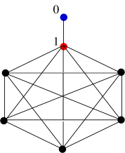
Figure 2: The graph $G_{6}$.

We consider the rumor scotching process on the graph $G_{n}$ on $\{0,\cdots,n\}$ obtained by adding on the complete graph on $\{1,\cdots,n\}$ the edge $(0,1)$, see Figure 2. Let ${\cal P}_{n}$ be the set of subsets of $\{0,\cdots,n\}$. With the notation in introduction, the rumor scotching process on $G_{n}$ is the Markov process on ${\cal X}_{n}=({\cal P}_{n}\times\{S,I,R\})^{n}$ with generator, for $X=(A_{i},s_{i})_{0\leq i\leq n}$,

$$K(X,X+E_{ij})=\lambda n^{-1}{\bf 1}(s_{i}=I){\bf 1}(s_{j}\neq R),$$

$$K(X,X-E_{j})={\bf 1}(s_{j}=I)\left(\sum_{i=1}^{n}{\bf 1}(i\in A_{j})\right),$$

and all other transitions have rate $0$. At time $0$, the initial state is $X(0)=(X_{i}(0))_{0\leq i\leq n}$ with $X_{0}(0)=(\emptyset,R)$, $X_{1}(0)=(\{0\},I)$ and for $i\geq 2$, $X_{i}(0)=(\emptyset,S)$.

With this initial condition, the process describes the propagation of a rumor started from vertex $1$ at time $0$. After an exponential time, vertex $1$ learns that the rumor is false and starts to scotch the rumor to the vertices it had previously informed. This process is a Markov process on a finite set with as absorbing states, all states without $I$-vertices. We define $N_{n}$ as the total number of recovered vertices when the process stops evolving. We also define $Y_{n}(t)$ as the distribution $N_{n}$ given that vertex $1$ is recovered at time $t$. We have the following

Theorem 4

• If $0<\lambda\leq 1/4$ and $t\geq 0$, as $n$ goes to infinity, $N_{n}$ and $Y_{n}(t)$ converge weakly respectively to $N$ and $Y(t)$ in the birth-and-assassination process of intensity $\lambda$.

• If $\lambda>1/4$, there exists $\delta>0$ such that

  $$\liminf_{n}{\mathrm{P}}_{\lambda}(N_{n}\geq\delta n)>0.$$

The proof of Theorem 4 relies on the convergence of the rumor scotching process to the birth-and-assassination process, exactly as the classical SIR dynamics converges to a branching process as the size of the population goes to infinity.

3.2 Proof of Theorem 4

3.2.1 Proof of Theorem 4(i)

The proof of Theorem 4 relies on an explicit contruction of the rumor scotching process. Let $(\xi^{(n)}_{ij}),1\leq i<j\leq n,$ be a collection of independent exponential variables with parameter $\lambda n^{-1}$ and, for all $1\leq i\leq j$, let $D_{ij}$ be an independent exponential variable with parameter $1$. We set $D_{ji}=D_{ij}$ and $\xi^{(n)}_{ji}=\xi^{(n)}_{ij}$. A network being a graph with marks attached on edges, we define ${\cal K}_{n}$ as the network on the complete graph of $\{1,\cdots,n\}$ where the mark attached on the edge $(ij)$ is the pair $(\xi_{ij}^{(n)},D_{ij})$. Now, the rumor scotching process is built on the network ${\cal K}_{n}$ by setting $\xi^{(n)}_{ij}$ as the time for the infected particle $i$ to infect the particle $j$ and $D_{ij}$ as the time for the recovered particle $i$ to recover the particle $j$ that it had previously infected.

The network ${\cal K}_{n}$ has a local weak limit as $n$ goes to infinity (see Aldous and Steele [3] for a definition of the local weak convergence). This limit network of ${\cal K}_{n}$ is ${\cal K}$, the Poisson weighted infinite tree (PWIT) which is described as follows. The root vertex, say $\emptyset$, has an infinite number of children indexed by integers. The marks associated to the edges from the root to the children are $(\xi_{i},D_{i})_{i\geq 1}$ where $\{\xi_{i}\}_{i\geq 1}$ is the realization of a Poisson process of intensity $\lambda$ on $\mathbb{R}_{+}$ and $(D_{i})_{i\geq 1}$ is a sequence of independent exponential variables with parameter $1$. Now recursively, for each vertex $i\geq 1$ we associate an infinite number of children denoted by $(i,1),(i,2),\cdots$ and the marks on the edges from $i$ to its children are obtained from the realization of an independent Poisson process of intensity $\lambda$ on $\mathbb{R}_{+}$ and a sequence of independent exponential variables with parameter $1$. This procedure is continued for all generations. Theorem 4.1 in [3] implies the local weak convergence of ${\cal K}_{n}$ to ${\cal K}$ (for a proof see Section 3 in Aldous [1]).

Now notice that the birth-and-assissination process is the rumor scotching process on ${\cal K}$ with initial condition: all vertices susceptible apart from the root which is infected and will be restored after an exponential time with mean $1$.

For $s>0$ and $\ell\in\mathbb{N}$, let ${\cal K}_{n}[s,\ell]$ be the network spanned by the set of vertices $j\in\{1,\cdots,n\}$ such that there exists a sequence $(i_{1},\cdots,i_{k})$ with $i_{1}=1$, $i_{k}=j$, $k\leq\ell$ and $\max(\xi^{(n)}_{i_{1}i_{2}},\cdots,\xi^{(n)}_{i_{k-1}i_{k}})\leq s$. If $\tau_{n}$ is the time elapsed before an absorbing state is reached, we get that ${\bf 1}(\tau_{n}\leq s){\bf 1}(N_{n}\leq\ell)$ is measurable with respect to ${\cal K}_{n}[s,\ell]$. From Theorem 4.1 in [3], we deduce that ${\bf 1}(\tau_{n}\leq s){\bf 1}(N_{n}\leq\ell)$ converges in distribution to ${\bf 1}(\tau\leq s){\bf 1}(N\leq\ell)$ where $\tau$ is the time elapsed before all particles die in the birth-and-assassination process. If $0<\lambda<1/4$, $\tau$ is almost surely finite and we deduce the statement (i).

3.2.2 Proof of Theorem 4(ii)

In order to prove part (ii) we couple the birth-and-assassination process and the rumor scotching process. We use the above notation and build the rumor scotching process on the network ${\cal K}_{n}$. If $X=((A_{i},s_{i})_{0\leq i\leq n})\in{\cal X}_{n}$, we define $I(X)=\{1\leq i\leq n:s_{i}=I\}$ and $S(X)=\{1\leq i\leq n:s_{i}=S\}$.

Let $X=X_{n}(u)\in{\cal X}_{n}$ be the state of the rumor scotching process at time $u\geq 0$. Let $i\in I(X)$, we reorder the variables $(\xi_{ij}^{(n)})_{j\in S(X)}$ in non-decreasing order: $\xi^{(n)}_{ij_{1}}\leq\cdots\leq\xi^{(n)}_{ij_{|S(X)|}}$. Define $\xi^{(n)}_{ij_{0}}=0$, from the memoryless property of the exponential variable, for $1\leq k\leq|S(X)|$, $\xi^{(n)}_{ij_{k}}-\xi^{(n)}_{ij_{k-1}}$ is an exponential variable with parameter $\lambda(|S(X)|-k+1)/n$ independent of $(\xi^{(n)}_{ij_{\ell}}-\xi^{(n)}_{ij_{\ell-1}}$, $\ell<k)$. Therefore, for all $1\leq k\leq|S(X)|$, the vector $(\xi^{(n)}_{ij_{1}},\cdots,\xi^{(n)}_{ij_{k}})$ is stochastically dominated component-wise by the vector $(\xi_{1},\cdots,\xi_{k})$ where $\{\xi_{j}\}_{j\geq 1}$ is a Poisson process of intensity $\lambda(|S(X)|-k+1)/n$ on $\mathbb{R}_{+}$ (i.e. for all $0\leq t_{1}\leq\cdots\leq t_{k}$, ${\mathrm{P}}(\xi^{(n)}_{ij_{1}}\geq t_{1},\cdots,\xi^{(n)}_{ij_{k}}\geq t_{k})\leq{\mathrm{P}}(\xi_{1}\geq t_{1},\cdots,\xi_{k}\geq t_{k})$). In particular if $|S(X)|\geq(1-\delta)n$, with $0<\delta<1/2$, then $(\xi^{(n)}_{i1},\cdots,\xi^{(n)}_{i\lfloor n\delta\rfloor})$ is stochastically dominated component-wise by the first $\lfloor n\delta\rfloor$ arrival times of a Poisson process of intensity $\lambda(1-2\delta)$.

Now, let $\delta>0$ such that $\lambda^{\prime}=\lambda(1-2\delta)>1/4$. We define $S^{(n)}_{u},I^{(n)}_{u},R^{(n)}_{u},$ as the number of $S,I,R$-particles at time $u\geq 0$ in ${\cal K}_{n}$, and $I^{\prime}_{u}$ as the number of particles ”at risk” at time $u$ in the birth-and-assassination process with intensity $\lambda^{\prime}$. Let $\tau_{n}=\inf\{u\geq 0:S^{(n)}_{u}\leq(1-\delta)n\}$. Note that if $0\leq u\leq\tau_{n}$ then any $I$-particle has infected less than $\lfloor\delta n\rfloor$ $S$-particles. From what precedes, we get

$$S^{(n)}_{u}{\bf 1}(u\leq\tau_{n})\leq_{st}n-I^{\prime}_{u}.$$

So that $S^{(n)}_{u}\leq_{st}\max(n-I^{\prime}_{u},(1-\delta)n)$. In particular, since $N_{n}\geq\sup_{u\geq 0}(n-S^{(n)}_{u})$, we get

$${\mathrm{P}}_{\lambda}(N_{n}\geq\delta n)\geq{\mathrm{P}}_{\lambda^{\prime}}(\limsup_{u\to\infty}I^{\prime}_{u}=\infty).$$

Finally, it is proved in [2] that if $\lambda^{\prime}>1/4$ then ${\mathrm{P}}_{\lambda^{\prime}}(\limsup_{u\to\infty}I^{\prime}_{u}=\infty)>0$.

References

- [1] D. Aldous. Asymptotics in the random assignment problem. Probab. Theory Related Fields, 93(4):507–534, 1992.
- [2] D. Aldous and W. Krebs. The “birth-and-assassination” process. Statist. Probab. Lett., 10(5):427–430, 1990.
- [3] D. Aldous and M. Steele. The objective method: probabilistic combinatorial optimization and local weak convergence. 110:1–72, 2004.
- [4] H. Andersson. Epidemic models and social networks. Math. Sci., 24(2):128–147, 1999.
- [5] K. Athreya and P. Ney. Branching processes. Springer-Verlag, New York, 1972.
- [6] O. Häggström and R. Pemantle. First passage percolation and a model for competing spatial growth. J. Appl. Probab., 35(3):683–692, 1998.
- [7] G. Kordzakhia. The escape model on a homogeneous tree. Electron. Comm. Probab., 10:113–124 (electronic), 2005.
- [8] G. Kordzakhia and S. P. Lalley. A two-species competition model on . Stochastic Process. Appl., 115(5):781–796, 2005.
- [9] M. Mitzenmacher. A brief history of generative models for power law and lognormal distributions. Internet Math., 1(2):226–251, 2004.
- [10] M. Newman, A.-L. Barabási, and D. J. Watts, editors. The structure and dynamics of networks. Princeton Studies in Complexity. Princeton University Press, Princeton, NJ, 2006.
- [11] K. Ramamritham and P. E. Shenoy. Special issue on dynamic information dissemination. IEEE Internet Computing, 11:14–44, 2007.
- [12] S. I. Resnick. Heavy-tail phenomena. Springer Series in Operations Research and Financial Engineering. Springer, New York, 2007. Probabilistic and statistical modeling.
- [13] D. Richardson. Random growth in a tessellation. Proc. Cambridge Philos. Soc., 74:515–528, 1973.
- [14] J. Tsitsiklis, C. Papadimitriou, and P. Humblet. The performance of a precedence-based queueing discipline. J. Assoc. Comput. Mach., 33(3):593–602, 1986.