Barnes slave boson approach to the two-site single impurity Anderson model with non-local interaction

Abstract

The Barnes slave boson approach to the $U=\infty$ single impurity Anderson model extended by a non-local Coulomb interaction is revisited. We demonstrate first that the radial gauge representation facilitates the treatment of such a non-local interaction by performing the exact evaluation of the path integrals representing the partition function, the impurity hole density and the impurity hole density autocorrelation function for a two-site cluster. The free energy is also obtained on the same footing. Next, the exact results are compared to their approximations at saddle-point level, and it is shown that the saddle point evaluation recovers the exact answer in the limit of strong non-local Coulomb interaction, while the agreement between both schemes remains satisfactory in a large parameter range.

Other nonperturbative techniques Strong-coupling expansions Strongly correlated electron systems; heavy fermions Field theory

1 Introduction

The amazing properties of transition metal oxides invite to consider a broad range of electronic applications. They also pose challenges to their explanation because certain properties cannot be addressed in a weak coupling scheme [1, 2]. Such properties include, for example, high temperature superconductivity, thermoelectricity in layered cobalt oxides, and colossal magnetoresistance in manganites. A promising theoretical framework for the elucidation of these phenomena is provided by Quantum Monte Carlo (QMC) approaches where the path integral representation of the corresponding models is handled on the level of a resummation of the corresponding Ising variables. Such simulations are successful in a limited parameter range only, excluding the strong coupling regime as recently discussed by Troyer and Wiese [3], while the inclusion of non-local interaction terms is problematic. Another tool for the study of such problems is dynamical mean-field theory (DMFT) where one maps the investigated Hubbard-type model on a single impurity Anderson model (SIAM) embedded in a self-consistent bath [4, 5, 6]. Although this was very successful for the study of the Mott transition, lattice effects are largely ignored in this approach. Current development points towards replacing the impurity by a cluster, again embedded in a self-consistent bath, as recently investigated in refs. [7, 8]. Since DMFT was developed for handling the onsite Coulomb interaction, long-ranged electron-electron interaction presents an additional challenge.

One alternative tool that can be applied to both impurity and lattice models is provided by the slave boson approach, which was pioneered by Barnes [9, 10] for the SIAM, and later on extended to the Hubbard model by Kotliar and Ruckenstein [11]. More recently the mean-field approach has been applied to a large variety of problems [12, 13, 14, 15, 16]. Even though such calculations can be systematically improved by means of a (partial) resummation of the loop expansion, few fluctuation calculations were effectively carried out [17, 18, 19]. This originates from the controversy on the implementation of the gauge symmetry [20, 17, 21], and other technical difficulties [22]. Nevertheless, using the Barnes slave boson approach in the radial gauge representation [23], the full resummation of the world lines was recently performed [24], and it was shown that the local density autocorrelation function, represented as a path integral, can be evaluated exactly for a small cluster. Furthermore, it has been demonstrated that the saddle-point amplitude of the slave boson field is not related to a Bose condensate. In this context, it is worth noting that one of the few analytical results obtained in the field of strongly correlated electron systems has been derived in this framework: for the $U=\infty$ Hubbard model and any bipartite lattice, the paramagnetic and fully polarised ferromagnetic ground states are degenerate at doping $1/3$ [25]. Though obtained on the Gutzwiller level, this result is in excellent agreement with subsequent careful numerical simulations [26].

The purpose of the present work is two-fold: first, we show that the exact evaluation of the path integrals representing expectation values and correlation functions can also be performed when a non-local Coulomb interaction is included. Second, for the considered model, we derive and compare mean-field to exact results to gain further insight into the validity of the saddle-point approximation of the slave boson formalism.

2 Interacting two-site cluster

2.1 Hamiltonian

The Hamiltonian of the interacting two-site cluster can be written as:

$${\mathcal{H}} = \sum_{\sigma}\left(c^{\dagger}_{\sigma}\epsilon_{\rm c}c^{\phantom{\dagger}}_{\sigma}+d^{\dagger}_{\sigma}\epsilon_{\rm d}d^{\phantom{\dagger}}_{\sigma}\right)+U\prod_{\sigma=\uparrow,\downarrow}d^{\dagger}_{\sigma}d^{\phantom{\dagger}}_{\sigma}$$ (1)

$$+ V\sum_{\sigma}\left(c^{\dagger}_{\sigma}d^{\phantom{\dagger}}_{\sigma}+{\rm h.c.}\right)+In_{\rm d}n_{\rm c},$$

where $U$ is the on-site repulsion, which is hereafter taken as infinite. The operators $c^{\dagger}_{\sigma}$ ($c^{\phantom{\dagger}}_{\sigma}$) and $d^{\dagger}_{\sigma}$ ($d^{\phantom{\dagger}}_{\sigma}$) describe the creation (annihilation) of the “band” electrons and impurity electrons respectively, with spin projection $\sigma$. The band and impurity energy levels are denoted by $\epsilon_{\rm c}$ and $\epsilon_{\rm d}$, while $V$ represents the hybridisation energy. The last term of eq. (1), ${\mathcal{H}}_{I}\equiv In_{\rm d}n_{\rm c}$, where $n_{\rm d}=\sum_{\sigma}d^{\dagger}_{\sigma}d^{\phantom{\dagger}}_{\sigma}$ and $n_{\rm c}$ is the density at the “band site”, represents the screened Coulomb interaction felt by an electron at the band site caused by an electron on the impurity.

Diagonalisation of the Hamiltonian of the two-site cluster, eq. (1), is straightforward, and all physical quantities of interest can be derived analytically [27]. Still, this model represents the simplest case where all terms in the Hamiltonian (1) play a significant role, justifying its investigation. A functional integral representation, which is appealing for its lack of spurious Bose condensation, is the slave boson representation in the radial gauge [23], based on the original representation by Barnes [9]. In the radial gauge, the path integral representation for slave bosons is defined on a discretised time mesh and the phase of the bosonic field is integrated out from the outset so that the underlying $U(1)$ gauge symmetry [28] is fully implemented. Accordingly, the original field $d^{\phantom{\dagger}}_{\sigma}$ is represented as:

$$d^{\phantom{\dagger}}_{n,\sigma}=\sqrt{x^{\phantom{\dagger}}_{n+1}}f^{\phantom{\dagger}}_{n,\sigma},\quad d^{\dagger}_{n,\sigma}=\sqrt{x^{\phantom{\dagger}}_{n}}f^{\dagger}_{n,\sigma},$$ (2)

where $x^{\phantom{\dagger}}_{n}$ and $x^{\phantom{\dagger}}_{n+1}$ are the slave boson field amplitudes at time steps $n$ and $n+1$, and $f^{\phantom{\dagger}}_{n,\sigma}$ the auxiliary fermion fields. The shift of one time step in the relation for $d^{\phantom{\dagger}}_{n,\sigma}$ is necessary to obtain a meaningful representation, as demonstrated in the case of the atomic limit [23]. This is the only non-trivial remainder of the normal order procedure.

2.2 Action

In order to implement the non-local Coulomb interaction in the Barnes slave boson approach (in the radial gauge), we first recast the corresponding contribution to the action as:

$$S_{I}=I\sum_{\sigma}\sum_{n=1}^{N}\delta\;c^{\dagger}_{n,\sigma}c^{\phantom{\dagger}}_{n-1,\sigma}(1-x^{\phantom{\dagger}}_{n}).$$ (3)

Here $n$ denotes the time steps, $\delta\equiv\beta/N$, with $\beta=1/k_{\rm B}T$ and $N$ the number of time steps. In this form the above term is bilinear in the fermionic fields. As a result, the action $S$ of the two-site cluster system may be written as the sum of a fermionic part, $S_{f}$, which is bilinear in the fermionic fields, and a bosonic part, $S_{b}$, with

$$S_{f} \equiv \sum_{\sigma}S_{f,\sigma}=\sum_{\sigma}\sum_{n}\left[c^{\dagger}_{n,\sigma}(c_{n,\sigma}-\Lambda_{n}c_{n-1,\sigma})\right.$$

$$\left.+f^{\dagger}_{n,\sigma}(f_{n,\sigma}-L_{\rm n}f_{n-1,\sigma})\right.$$

$$\left.+V\delta~{}\sqrt{x_{n}}(c^{\dagger}_{n,\sigma}f_{n-1,\sigma}+f^{\dagger}_{n,\sigma}c_{n-1,\sigma})\right],\phantom{\sum_{N}}$$

$$S_{b} = \sum_{n}\left[i\delta\lambda_{n}(x_{n}-1)\right]$$ (4)

where $\Lambda_{n}=e^{-\delta(\epsilon_{\rm c}-\mu+I(1-x^{\phantom{\dagger}}_{n}))}\equiv L_{\rm c}e^{-\delta I(1-x^{\phantom{\dagger}}_{n})}$, $L_{n}=e^{-\delta(\epsilon_{\rm d}-\mu+i\lambda_{n})}\equiv L_{\rm d}~{}e^{-i\delta\lambda_{n}}$, and $\lambda_{n}$ is the time-dependent constraint field. Here, the physical electron creation (annihilation) operator is represented using eq. (2). Note that the non-local interaction term is incorporated into the local potential term of the $c$-field, which becomes time-dependent. Besides, $S_{f}$ ($S_{f,\sigma}$) is bilinear in the fermionic fields, and the corresponding matrix of the coefficients will be denoted as $\left[S\right]$ ($\left[S_{\sigma}\right]$). The above form cannot be obtained by transformations of the conventional integral in the Cartesian gauge without invoking assumptions. Therefore, the above treatment is specific to radial slave bosons for which phase variables are entirely absent [23]. Accordingly, there is no $U(1)$ symmetry breaking associated to a saddle-point approximation.

2.3 Partition function and free energy

The path integral representation of the partition function of the two-site cluster [23] may be formulated equivalently as the projection of the determinant of a fermionic matrix:

$${\mathcal{Z}} = \lim_{\begin{subarray}{c}N\rightarrow\infty\\ \epsilon\rightarrow 0^{+}\end{subarray}}\left(\prod_{n=1}^{N}\int\prod_{\sigma}D[f_{n,\sigma},f^{\dagger}_{n,\sigma}]D[c_{n,\sigma},c^{\dagger}_{n,\sigma}]\;\times\right.$$ (5)

$$\left.\int_{-\infty}^{\infty}\frac{\displaystyle\delta{\rm d}\lambda_{n}}{\displaystyle 2\pi}\int_{-\epsilon}^{\infty}{\rm d}x_{n}\right)e^{-S}$$

$$= \lim_{\begin{subarray}{c}N\rightarrow\infty\\ \epsilon\rightarrow 0^{+}\end{subarray}}{\mathcal{P}_{1}}\ldots{\mathcal{P}_{N}}~{}\mbox{det}\left[S\right],$$

where $\mbox{det}\left[S\right]$ is the determinant of the matrix representation of the action $S$, eq. (2.2), in the basis $\{c_{n,\sigma},f_{n,\sigma}\}$. The operator ${\mathcal{P}}_{n}$ is defined as:

$${\mathcal{P}}_{n}=\int_{-\infty}^{+\infty}\delta~{}\frac{\displaystyle{\rm d}\lambda_{n}}{\displaystyle 2\pi}~{}\int_{-\epsilon}^{+\infty}{\rm d}x_{n}~{}e^{-\delta\left[i\lambda_{n}(x_{n}-1)\right]},$$ (6)

for all $n$, and acts as a projector from the enlarged Fock space “spanned” by the auxiliary fields down to the physical space. The action of these projectors on the various contributions resulting from $\mbox{det}\left[S\right]$ are given explicitly in table 1. Alternative expressions of the projectors ${\mathcal{P}}_{n}$ exist [23, 24]. However the properties given in table 1 are independent of the particular form of ${\mathcal{P}}_{n}$. No further properties of ${\mathcal{P}}_{n}$ are needed for our purpose.

In the absence of nearest-neighbour interaction, the calculation of the partition function was performed for the spinless and spin 1/2 systems in ref. [24]. It builds on the rewriting of the fermionic determinant into a convenient diagonal-in-time form, which, if we include the nearest-neighbour interaction and first focus on the spinless case, reads:

$$\mbox{det}\left[S_{\sigma}\right]=\mbox{Tr}\prod_{n}\left[{\mathcal{K}}_{I,n}\right],$$ (7)

where,

$$\left[{\mathcal{K}}_{I,n}\right]=\left(\begin{array}[]{cccc}1&{}\hfil&{}\hfil&{}\hfil\\ {}\hfil&\Lambda_{n}&\delta V\sqrt{x_{n}}&{}\hfil\\ {}\hfil&\delta V\sqrt{x_{n}}&L_{n}&{}\hfil\\ {}\hfil&{}\hfil&{}\hfil&\Lambda_{n}L_{n}\end{array}\right).$$ (8)

This expression follows from recursion relations that are established when determining the fermionic determinant. We thus obtain the partition function as

$${\mathcal{Z}}_{0}=\lim_{\begin{subarray}{c}N\rightarrow\infty\\ W\rightarrow\infty\end{subarray}}{\mathcal{P}_{1}}\ldots{\mathcal{P}_{N}}~{}\mbox{Tr}\prod_{n=1}^{N}\left[{\mathcal{K}}_{I,n}\right].$$ (9)

Since the time steps are now decoupled, ${\mathcal{Z}}_{0}$ can be explicitly evaluated using the properties listed in table 1.

Remarkably, the extension to spin 1/2 is straightforward: the partition function is also given by eq. (9), under the replacement of the matrix $\left[{\mathcal{K}}_{I,n}\right]$ by $\left[{\mathcal{K}}_{I,n}\right]\otimes\left[{\mathcal{K}}_{I,n}\right]$, where these two factors follow from the two spin projections. Accordingly, the dimension of the Fock space increases from four to sixteen. It effectively reduces to twelve in the $U=\infty$ limit. Higher spins can be handled in a similar fashion.

As an example let us consider the two-electron case, where all interaction terms are relevant. Using the results of table 1 we obtain

$$\!\!\!\!\!\!\!\!\!\!\!\left[k_{I}\right]\equiv{\mathcal{P}}_{n}(\left[{\mathcal{K}}_{I,n}\right]\otimes\left[{\mathcal{K}}_{I,n}\right])=\phantom{\int_{N}^{N}}$$ (10)

$$\left(\begin{array}[]{ccccc}L_{\rm c}^{2}&L_{\rm c}\delta V&L_{\rm c}\delta V&&\\ L_{\rm c}\delta V&L_{\rm c}L_{\rm d}e^{-\delta I}&0&&\\ L_{\rm c}\delta V&0&\!\!\!\!L_{\rm c}L_{\rm d}e^{-\delta I}&&\\ &&&\!\!\!\!\!\!L_{\rm c}L_{\rm d}e^{-\delta I}&\\ &&&&\!\!\!\!\!\!L_{\rm c}L_{\rm d}e^{-\delta I}\end{array}\right)$$ (16)

Table 1: Action of projectors ${\mathcal{P}}_{n}$ on a factor ${\mathcal{F}}$. Here $q$ is real positive.

${\mathcal{F}}$	$x_{n}^{q}$	$e^{i\delta\lambda_{n}}$	$L_{n}x_{n}$	$L_{n}^{2}$	$\Lambda_{n}^{q}$	$\Lambda_{n}L_{n}$	$\Lambda_{n}x_{n}$
${\mathcal{P}}_{n}$ $\cdot$ ${\mathcal{F}}$	1	1	0	0	$L_{{\rm c}}^{q}$	$L_{{\rm c}}L_{{\rm d}}e^{-\delta I}$	$L_{{\rm c}}$

When diagonalising $\left[k_{I}\right]$ we obtain a three-fold degenerate eigenvalue $\lambda^{(t)}$ corresponding to the triplet states, and two eigenvalues $\lambda_{\pm}^{(s)}$ corresponding to the singlet states. The latter two read:

$$\lambda_{\pm}^{(s)}=\frac{L_{\rm c}}{2}\left[L_{\rm c}+L_{\rm d}e^{-\delta I}\pm\sqrt{\left(L_{\rm c}-L_{\rm d}e^{-\delta I}\right)^{2}+8\left(\delta V\right)^{2}}\right]$$ (17)

Then, with $\Delta\equiv\epsilon_{\rm c}-\epsilon_{\rm d}$, straightforward manipulations yield the correct free energy at zero temperature as:

$$F=\frac{1}{2}\left(3\epsilon_{\rm c}+\epsilon_{\rm d}+I-\sqrt{(\Delta-I)^{2}+8V^{2}}\right).$$ (18)

3 Impurity hole density and autocorrelation function

Let us now determine the expectation value of the amplitude of the slave boson field at time step $m$, $\langle x_{m}\rangle$. A first guess for $\langle x_{m}\rangle$ would be $\langle x_{m}\rangle=0$, invoking Elitzur’s theorem [29]. However, one should remember that in our approach the phase of the boson has been gauged away from the outset, and therefore the phase fluctuations, that suppress $\langle x_{m}\rangle$ to zero, are absent. Instead, $\langle x_{m}\rangle$ does represent the hole density on the impurity site $1-n_{\rm d}(m\delta)$ in the introduced path integral formalism. The impurity hole density is given by:

$${\mathcal{Z}}\langle x_{m}\rangle = \lim_{\begin{subarray}{c}N\rightarrow\infty\\ \epsilon\rightarrow 0^{+}\end{subarray}}{\mathcal{P}_{1}}\ldots{\mathcal{P}_{N}}~{}\left(\mbox{det}\left[S\right]~{}x_{m}\right)$$

$$= \lim_{\begin{subarray}{c}N\rightarrow\infty\\ \epsilon\rightarrow 0^{+}\end{subarray}}{\mathcal{P}_{1}}\ldots{\mathcal{P}_{N}}~{}\left(x_{m}\mbox{Tr}~{}\prod_{n=1}^{N}\left[{\mathcal{K}}_{I,n}\right]\otimes\left[{\mathcal{K}}_{I,n}\right]\right).$$

In addition to the matrix $\left[k_{I}\right]$, we define the hole-weighted matrix $\left[{\mathcal{K}}_{I,X}\right]\equiv{\mathcal{P}}_{n}(x_{n}\left[{\mathcal{K}}_{I,n}\right]\otimes\left[{\mathcal{K}}_{I,n}\right])$ for all $n$ so that eq. (3) becomes:

$${\mathcal{Z}}\langle x_{m}\rangle=\lim_{N\rightarrow\infty}\mbox{Tr}\left(\left[{\mathcal{K}}_{I,X}\right]\left[k_{I}\right]^{N-1}\right).$$ (20)

In the limit $\delta\rightarrow 0$, the matrix $\left[{\mathcal{K}}_{I,X}\right]$ reduces to the representation of the hole density operator in Fock space as one would write it in the Hamiltonian language:

$$\left[{\mathcal{K}}_{I,X}\right]_{i,j}=\delta_{i,1}\delta_{j,1}.$$ (21)

At this stage the impurity hole density can be determined using eqs. (20) and (21) and we find:

$$\;\;\;\;\;\;\langle x_{m}\rangle=\langle x\rangle=\frac{8V^{2}}{\left(\Delta-I+\sqrt{(\Delta-I)^{2}+8V^{2}}\right)^{2}+8V^{2}}.$$ (22)

Note that $\langle x\rangle$ vanishes for $\Delta\rightarrow\infty$, but this suppression does not result from phase fluctuations. For $I\rightarrow\infty$ and finite $\Delta$, the correct limit $\langle x\rangle\rightarrow 1$ is approached.

Figure 1: Hole occupation $\langle x\rangle$ as function of $\epsilon_{\rm c}-\epsilon_{\rm d}=\Delta$, in units of $V$, for various values of the interaction strength $I$. (a) mean-field result, and (b) exact result.

In this framework the calculation of the hole density autocorrelation function can be carried out in a similar fashion, with the result:

$${\mathcal{Z}}\langle x_{1}x_{m}\rangle=\lim_{N\rightarrow\infty}\mbox{Tr}\left(\left[k_{I}\right]^{N-m}\left[{\mathcal{K}}_{I,X}\right]\left[k_{I}\right]^{m-2}\left[{\mathcal{K}}_{I,X}\right]\right).$$ (23)

Introducing the eigenvalues $\lambda_{\pm}^{(s)}$ and eigenvectors of $\left[k_{I}\right]$, eq. (10) and eq. (17), the evaluation is straightforward as only the first component of the two eigenvectors in the singlet subspace contributes to eq. (23). They are given by:

$$\alpha_{\pm}=\frac{8V^{2}}{8V^{2}+\left(\Delta-I\pm\sqrt{\left(\Delta-I\right)^{2}+8V^{2}}\right)^{2}}\;.$$ (24)

The calculation yields:

$${\mathcal{Z}}\langle x_{1}x_{m}\rangle = \alpha_{+}^{4}\lambda_{+}^{N-2}+\alpha_{-}^{4}\lambda_{-}^{N-2}$$

$$+ \left(\alpha_{+}\alpha_{-}\right)^{2}\left[\lambda_{+}^{N-m}\lambda_{-}^{m-2}+\lambda_{-}^{N-m}\lambda_{+}^{m-2}\right].$$

In this form we clearly recognise the standard expression of a correlation function: the matrix elements of the hole density operator in the basis of the eigenstates of the Hamiltonian are represented by $\alpha_{\pm}$, the Boltzmann weights by $\lambda_{\pm}^{N}/{\mathcal{Z}}$, and the dynamical factors by $\left(\lambda_{\pm}/\lambda_{\mp}\right)^{m}$. Note that we obtain the full correlation function, including static terms. In the zero-temperature limit, using $\lim_{N\rightarrow\infty}\lambda_{\pm}^{-2}=1$, the hole density autocorrelation function finally reads:

$$\langle x_{1}x_{m}\rangle=\langle x\rangle^{2}+\left(\alpha_{+}\alpha_{-}\right)^{2}\left[\left(\frac{\lambda_{-}}{\lambda_{+}}\right)^{m}+\left(\frac{\lambda_{-}}{\lambda_{+}}\right)^{N-m}\right]$$ (26)

where the static term has been reshaped using eq. (22). The correlation function may be cast into an exponential form for sufficiently large $m$ and $N-m$.

4 Comparison of saddle-point approximation and exact slave boson evaluation

The slave boson saddle-point approximation to the Hubbard model has been used in a variety of cases [12, 13, 14, 15, 16, 25], and we further test it in the framework of the single impurity Anderson model with non-local Coulomb interaction.

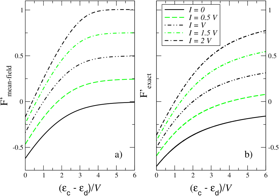
Figure 2: Site normalised free energy $F^{\prime}\equiv(F-\epsilon_{\rm c}-\epsilon_{\rm d})/2$ as a function of $\epsilon_{\rm c}-\epsilon_{\rm d}$, in units of $V$, for various values of the interaction strength $I$. (a) mean-field result, and (b) exact result.

4.1 Slave boson saddle-point results

On the saddle-point approximation level, we obtain the grand potential as:

$$\Omega_{\rm MF}=-T\sum_{\rho,\sigma}\ln{\left(1+e^{-\beta E_{\rho,\sigma}}\right)}-\lambda_{0}(1-x)\;,$$ (27)

where $x$ and $\lambda_{0}$ represent the saddle-point approximation of the corresponding fields. The two eigenvalues of the fermionic matrix read:

$$E_{\rho,\sigma} = \frac{1}{2}\left(\epsilon_{\rm c}+I(1-x)+\epsilon_{\rm d}+\lambda_{0}-2\mu\right.$$

$$\left.+\rho\sqrt{\left(\epsilon_{\rm d}+\lambda_{0}-\epsilon_{\rm c}-I(1-x)\right)^{2}+4xV^{2}}\right),$$

and $\rho=\pm 1$. If one now again focuses on the two-electron case, $\lambda_{0}$ can be expressed in terms of $\Delta$, $I$, and $x$ as

$$\lambda_{0}=\Delta+I(1-x)+2xV\sqrt{\frac{x}{1-x^{2}}}$$ (29)

where $x$ satisfies

$$2V(1-3x^{2})=\sqrt{x(1-x^{2})}\left(\Delta-2Ix\right).$$ (30)

There are two limits in which the solution of this equation takes a simple form. First, for $I\gg V$ and $\Delta=0$ we obtain

$$x=1-2\left(\frac{V}{I}\right)^{2}+{\mathcal{O}}\left(\left(\frac{V}{I}\right)^{4}\right)$$ (31)

and second, for $I\rightarrow 0$ and $\Delta\gg V$, the solution reads:

$$x=\left(\frac{2V}{\Delta}\right)^{2}+{\mathcal{O}}\left(\left(\frac{V}{\Delta}\right)^{4}\right)\,.$$ (32)

If one now compares the above results to eq. (22) one realises that eq. (31) represents the exact result, while eq. (32) differs from it by a factor 2. We thus have identified another regime where the slave boson mean-field approach yields an (at least partly) exact answer.

In the intermediate regime of the interaction strength $I$, the solution of eq. (30) is shown in fig. 1(a). For decreasing $I$, the hole occupation on the impurity decreases rapidly, especially for small $\Delta$. In contrast, for large $\Delta$, $I$ plays a lesser role as can be read from eq. (30), and all curves rapidly merge in the result given by eq. (32). This reproduces the trends exhibited by the exact solution shown in fig. 1(b). Strikingly, the agreement between the approximate and exact solutions is already excellent for $I=2V$ and $\Delta=0$, and improves for increasing $I$. However, substantial discrepancies are found for decreasing $I$ or increasing $\Delta$.

In order to further investigate the quality of the mean-field solution we turn now to the free energy. It reads:

$$F_{\rm MF}=\epsilon_{\rm c}+\epsilon_{\rm d}+\lambda_{0}x+I(1-x)-2V\sqrt{\frac{x}{1-x^{2}}}\,.$$ (33)

For large $I$ and $\Delta=0$, where the mean-field approach produced the exact answer for $\langle x\rangle$, we obtain from the mean-field solutions eq. (29) and eq. (31):

$$F_{\rm MF}=2\epsilon_{\rm d}-2V\left(\frac{V}{I}\right)^{3}+V{\mathcal{O}}\left(\left(\frac{V}{I}\right)^{5}\right)\,.$$ (34)

Surprisingly, this does not account for the correct dependence on $V/I$, which is given by:

$$F_{\rm exact}=2\epsilon_{\rm d}-2I\left(\frac{V}{I}\right)^{2}+I{\mathcal{O}}\left(\left(\frac{V}{I}\right)^{4}\right)\,.$$ (35)

In this case, while the saddle-point approximation to $\langle x\rangle$ yields the exact result, this is not valid for the free energy.

If we now turn to the case $\Delta-I\gg V$ the free energy reads:

$$F_{\rm MF}=\epsilon_{\rm c}+\epsilon_{\rm d}+I+{\mathcal{O}}\left(\frac{V^{3}}{\Delta^{2}}\right)$$ (36)

as the corrections of order ${\mathcal{O}}\left(\frac{V}{\Delta}\right)$ vanish. In this regime, expanding the exact result eq. (18) to leading order in $V/(\Delta-I)$, yields

$$F_{\rm exact}=\epsilon_{\rm c}+\epsilon_{\rm d}+I-\frac{2V^{2}}{\Delta-I}\,+{\mathcal{O}}\left(\frac{V^{4}}{(\Delta-I)^{3}}\right).$$ (37)

Therefore, the mean-field result correctly reproduces the large $\Delta$ limit, but fails at leading order in $V/\Delta$.

Between these two regimes one observes in fig. 2(a) that the mean-field free energy increases monotonically with $\Delta$ and $I$, rapidly saturating to its $\Delta\rightarrow\infty$ value. The lack of a ${\mathcal{O}}\left(\frac{V^{2}}{\Delta}\right)$ correction is clearly visible when comparing to the exact solution shown in fig. 2(b). While the discrepancies are rather moderate for $\Delta=0$ and large $I/V$, and for $\Delta\rightarrow\infty$, they increase in the intermediate regime.

5 Conclusion

In this work we applied the slave boson path integral formalism to an Anderson impurity model extended with a non-local Coulomb interaction. In general, the non-local terms of the Hamiltonian make the direct evaluation of the functional integrals impossible. We have demonstrated here the distinct advantage of using the radial gauge representation for the slave boson to address such a problem: $i/$ non-local Coulomb interaction terms can easily be incorporated into the calculation of the path integrals owing to the fact that the corresponding contribution to the action is bilinear in the fermionic fields, and $ii/$ when the band consists of a few sites only, a variety of quantities in the path integral formalism can be exactly calculated. For the simple two-site case, we determined the partition function from which the free energy was immediately derived. We also evaluated exactly the local hole density and hole density autocorrelation function. The former, expressed as $\langle x\rangle$, is generically finite, and is not related to the Bose condensation of the Barnes slave boson. Therefore, its evaluation on the saddle-point level is meaningful. When compared, the expectation value and its saddle-point approximation coincide in the regime $I\gg V$ and $\Delta=0$. Moreover, the mean-field free energy coincides with its exact evaluation in that case, while it only captures the correct limit for $\Delta\rightarrow\infty$. It seems unlikely that increasing the number of sites is going to significantly affect the quality of the saddle-point approximation, though this needs to be verified rigorously. Work along this line is in progress.

- [1] \NameLee P.A., Nagaosa N. Wen X.G. \REVIEWRev. Mod. Phys.78200617.
- [2] \NameMaekawa S., Tohyama T., Barnes S.E., Ishihara S., Koshibae W. Khaliullin G. Physics of Transition Metal Oxides (Springer Verlag, Berlin, 2004).
- [3] \NameTroyer M. Wiese U. \REVIEWPhys. Rev. Lett.942005170201.
- [4] \NameGeorges A., Kotliar G., Krauth W. Rozenberg M. \REVIEWRev. Mod. Phys.68199613.
- [5] \NameMetzner W. Vollhardt D. \REVIEWPhys. Rev. Lett.621989324.
- [6] \NameMaier T., Jarrel M., Pruschke T. Hettler M.H. \REVIEWRev. Mod. Phys.7720051027.
- [7] \NameKyung B., Kotliar G. Tremblay A.-M. S. \REVIEWPhys. Rev. B73200673.
- [8] \NameTremblay A.-M. S., Kyung B. Sénéchal D. \REVIEWFizika Nizkikh Temperatur322006561 [\REVIEWLow Temp. Phys.322006424].
- [9] \NameBarnes S.E. \REVIEWJ. Phys. F: Metal Phys.619761375.
- [10] \NameBarnes S.E. \REVIEWJ. Phys. F: Metal Phys.719772637.
- [11] \NameKotliar G. Ruckenstein A.E. \REVIEWPhys. Rev. Lett.57198657.
- [12] \NameLilly L., Muramatsu A. Hanke W. \REVIEWPhys. Rev. Lett.6519901379.
- [13] \NameFrésard R., Dzierzawa M. Wölfle P. \REVIEWEurophys. Lett.151991325.
- [14] \NameYuan Q. Kopp T. \REVIEWPhys. Rev. B652002085102.
- [15] \NameSeibold G., Sigmund E. Hizhnyakov V. \REVIEWPhys. Rev. B5719986937.
- [16] \NameRaczkowski M., Frésard R. Oleś A.M. \REVIEWPhys. Rev. B732006174525.
- [17] \NameBang Y., Castellani C., Grilli M., Kotliar G., Raimondi R. Wang Z. \REVIEWInt. J. of Mod. Phys. B61992531.
- [18] \NameZimmermann W., Frésard R. Wölfle P. \REVIEWPhys. Rev. B56199710097.
- [19] \NameKoch E. \REVIEWPhys. Rev. B642001165113.
- [20] \NameJolicœur Th. Le Guillou J.C. \REVIEWPhys. Rev. B4419912403.
- [21] \NameFrésard R. Wölfle P. \REVIEWInt. J. of Mod. Phys. B61992685; Erratum, \REVIEWInt. J. of Mod. Phys. B619923087.
- [22] \NameArrigoni E., Castellani C., Grilli M., Raimondi R. Strinati G.C. \REVIEWPhys. Rep.2411994291.
- [23] \NameFrésard R. Kopp T. \REVIEWNucl. Phys. B5942001769.
- [24] \NameFrésard R., Ouerdane H. Kopp T. \REVIEWNucl. Phys. B7852007286.
- [25] \NameMöller B., Doll K. Frésard R. \REVIEWJ. Phys.: Condens. Matter519934847.
- [26] \NameBecca F. Sorella S. \REVIEWPhys. Rev. Lett.8620013396.
- [27] The exact result for can be found in \NameA.C. Hewson The Kondo Problem to Heavy Fermions, Appendix C, Cambridge University Press, Cambridge (1997).
- [28] \NameRead N. Newns D.M. \REVIEWJ. Phys. C1619833273.
- [29] \NameElitzur S. \REVIEWPhys. Rev. D1219753978.