Can photo-ionisation explain the decreasing fraction of X-ray obscured AGN with luminosity?

Chandra and XMM-Newton surveys show that the fraction of obscured AGN decreases rapidly with increasing luminosity. Although this is usually explained by assuming that the covering factor of the central engine is much smaller at luminous QSOs, the exact origin of this effect remains unknown. We perform toy simulations to test whether photo-ionisation of the obscuring screen in the presence of a strong radiation field can reproduce this effect. In particular, we create X-ray spectral simulations using a warm absorber model assuming a range of input column densities and ionisation parameters. We fit instead the simulated spectra with a simple cold absorption power-law model that is the standard practice in X-ray surveys. We find that the fraction of absorbed AGN should fall with luminosity as $L^{-0.16\pm 0.03}$ in rough agreement with the observations. Furthermore, this apparent decrease in the obscuring material is consistent with the dependence of the FeK$\alpha$ narrow-line equivalent width on luminosity, ie. the X-ray Baldwin effect.

1 INTRODUCTION

The deepest Chandra X-ray surveys find a high surface density of AGN (Alexander et al. 2003, Giacconi et al. 2002). At the faintest fluxes probed, $\rm f_{X}(2-10keV)\approx 10^{-16}$ $\rm erg\leavevmode\nobreak\ cm^{-2}\leavevmode\nobreak\ s^{-1}$, the large majority of these sources ($\sim$ 80%) are obscured, having a hydrogen column density of $\rm N_{H}>10^{22}$ $\rm cm^{-2}$(e.g. Akylas et al. 2006; Tozzi et al. 2006). The high fraction of obscured AGN witnessed by Chandra is well in agreement with previous X-ray background synthesis models (e.g. Comastri et al. 1995, 2001). However, the situation is drastically different at the brighter fluxes probed by the XMM-Newton surveys. These show a marked deficit of X-ray obscured AGN (Piconcelli et al. 2002; Perola et al. 2004; Georgantopoulos et al. 2004; Caccianiga et al. 2004). The fraction of the obscured AGN drops to $\sim 30\%$ at fluxes of $\rm f_{X}(2-10\leavevmode\nobreak\ keV)\approx 10^{-14}$ $\rm erg\leavevmode\nobreak\ cm^{-2}\leavevmode\nobreak\ s^{-1}$. In flux limited samples, a small increase in the obscured AGN fraction with decreasing observed flux is expected, as the absorbed sources present lower flux. However the observed increase is much steeper than that predicted (eg. Piconcelli et al. 2002).

This discrepancy has been resolved with recent Chandra and XMM-Newton observations (e.g. Akylas et al. 2006; La Franca et al. 2005; Ueda et al. 2003) which demonstrate that the X-ray obscured AGN fraction is lower at higher luminosities. This can also explain the deficit of type-2 narrow-line QSOs at high redshift (Steffen et al. 2003). Recent X-ray background synthesis models that take into account the dependency of the obscured AGN fraction on luminosity (Gilli, Comastri & Hasinger 2007) are very successful in predicting the observed flux distribution.

The important question is what is the physical mechanism that can produce the decrease in the fraction of obscured AGN. It is possible that in the presence of a strong radiation field the fraction covered by the torus may be reduced. Köningl & Kartje (1994) for example proposed a disc-driven hydromagnetic wind model of the torus where for high bolometric luminosities the radiation pressure is expected to flatten the torus. A similar model, the receding torus model, has been invoked by Lawrence (1991) and Simpson (2005), to explain the fraction of radio AGN optically classified as type-2. In the presence of a strong radiation field the dust is heated and sublimates when it reaches a temperature of about 1500-2000K. At high luminosities the sublimation radius increases and thus effectively the torus opening angle increases, resulting in a higher number of type-1 AGN.

A similar effect is expected to take place in X-ray wavelengths. The X-ray absorbing gas is situated close to the nucleus as inferred from X-ray variability studies of type-2 AGN (Risaliti, Elvis & Nicastro 2002). Thus it is reasonable to assume that a strong radiation field will also ionise an appreciable fraction of the surrounding obscuring screen, resulting in the decrease in the “effective” column density. In this paper, we perform toy X-ray spectral simulations to estimate the strength of this effect. We also discuss any possible connection with the X-ray Baldwin effect.

2 X-ray Simulations

2.1 Simulation Description

We assume a constant $n_{e}r^{2}$ relation for all AGN, where $n_{e}$ and $r$ are the density of the obscuring screen and its distance from the nucleus respectively. This choice ensures a uniform ionisation state for the circumnuclear material i.e. the ionisation parameter $\xi$(=L/n_er² ergs cm s^-1) is the same at all distances from the nucleus. This could also imply that at a given distance from the central Black Hole the density is roughly the same in all AGN. Although this may not be the case, it is indirectly supported by the observational estimates for the density of the Broad Line Region (BLR) suggesting a uniform value of $\sim$10⁹ cm^-3 (Peterson 2006) across a large number of nearby AGN.

We use the XSPEC v12.0 package (Arnaud 1996) to generate 1000 simulated Chandra spectral files according to the following specifications:

1. A power-law model modified by an ionised absorber (ABSORI model, Done et al. 1992) with a photon index fixed to 1.9 (Nandra & Pounds 1994).

2. A redshift of 0.8 that corresponds to the peak redshift in the deep Chandra X-ray fields (e.g. Tozzi et al. 2006) and thus the average redshift of the sources that produce the X-ray background.

3. An amount of $N_{H}$ randomly varying in the range of $10^{21}-10^{24}$ cm^-2. We use a ratio of obscured ($N_{H}>10^{22}$ cm^-2 ) to unobscured ($N_{H}<10^{22}$ cm^-2 ) sources of 4:1 that is similar to that observed in the Chandra deep fields at the lowest flux levels (e.g. Akylas et al. 2006, Tozzi et al. 2006). We further assume, a flat distribution of $N_{H}$ in the 10²² to 10²⁴ cm^-2 region.

4. An ionisation parameter, $\xi$=L/n_er² ergs cm s^-1, (where L is the source luminosity in the 13.6 eV to 13.6 keV bandpass), randomly varying between 0 and 1000.

5. An arbitrary combination of an intrinsic 2-8 keV flux of $\sim 10^{-14}$ $\rm erg\leavevmode\nobreak\ cm^{-2}\leavevmode\nobreak\ s^{-1}$ and an exposure time of 50 ks to ensure a minimum of 10 counts per spectrum regardless of the $N_{H}$ and $\xi$ values.

These files are then fitted in XSPEC, using a power-law model modified by a cold photoelectric absorption model (WA*PO) to estimate the “effective” neutral column density. We consider only the 0.3-8 keV energy band in the spectral fits where the Chandra effective area is high. Sources with adequate photon statistics ($>$ 100 counts) are fitted using the $\chi^{2}$ statistic while for sources with less than 100 counts we use the most appropriate C-statistic technique (Cash 1979). We compare the parent and measured column density distribution in Fig. 1. The solid line histogram describes the input $N_{H}$ distribution assumed in the simulation (ABSORI*PO model) and the short dashed line the output one (WA*PO model). Note that due to the poissonian errors in each $N_{H}$ bin the shape of input $N_{H}$ slightly deviates from the assumed one. Clearly, there is a significant reduction in the number of obscured ($N_{H}>10^{22}$ cm^-2) sources in comparison to the initial distribution.

Figure 1: The solid line histogram describes the input $N_{H}$ distribution used for the warm absorption simulations and the short dashed line the output one, after fitting the simulated data with a cold absorption power-law model.

2.2 The simulated spectra

An important question that arises is whether the typical X-ray surveys such as carried out by Chandra or XMM-Newton can discriminate between a photo-ionised (i.e. ABSORI model) and a neutral absorption model (i.e. WA model) given the observational limitations i.e. the limited signal-to-noise ratio and energy resolution. The answer to this question depends primarily on the spectrum quality in the sense that in the sources with many counts we can more easily reject the neutral absorption model based on the $\chi^{2}$ statistic result. The amount of the $N_{H}$ and its degree of ionisation $\xi$ also play an important role given that their value may cause more or less prominent ionisation features to appear in the X-ray spectrum.

To explore this we examine two different samples, each one representative of our simulation, containing $\sim$100 sources each. These sets present $\sim$100 and $\sim$500 counts respectively in their 0.3-8 keV spectrum. In Fig. 2 we present the distribution of the best reduced $\chi^{2}$ values ($\chi^{2}_{\nu}$) when fitting the data using a cold absorption power-law model with $\Gamma$ fixed to 1.9.

Figure 2: The distribution of the $\chi^{2}_{\nu}$ values for the “low count” (dotted line) and the “high count” (solid line) samples.

Both distributions presented in this figure peak around $\chi^{2}_{\nu}$$\sim 1$ while the high count distribution is shifted to higher $\chi^{2}_{\nu}$ values in respect to the low count distribution. Furthermore these histograms suggest that the $\sim$85 percent of the low count and the $\sim$75 per cent of the high count sources would give an acceptable statistical result when fitted using a simple absorbed power law model (a value of 1 of the $\chi^{2}_{\nu}$ implies that the adopted model has an acceptance probability of 0.4 for 20 degrees of freedom). Only in a few cases the cold absorption power-law model could be automatically rejected based on the $\chi^{2}_{\nu}$ value (e.g. $\chi^{2}_{\nu}\sim 2$ implies that the cold absorption power-law model is rejected at $\sim 3\sigma$ confidence level for 20 degrees of freedom). In Fig. 3 we present some characteristic high-count simulated spectra. Table 1 summarises the spectral fitting results.

Figure 3: Characteristic spectra from the high-count simulated sample. We present two different $N_{H}$ values, namely 10²³ and 5$\times$10²³ cm^-2 in four different ionisation states (i.e. $\xi$=1, 100, 1000 & 5000).

Table 1: Spectral fitting results for the eight example simulated spectra presenting in Fig 3

${N_{H_{in}}}^{a}$	$\xi^{b}$	$\Gamma^{c}$	${N_{H_{out}}}^{d}$	$\chi^{2}/d.o.f^{e}$
$\times 10^{22}$ cm-2	ergs cm s-1		$\times 10^{22}$ cm-2
10	1	1.9	$9.2^{+0.8}_{-0.9}$	18.9/22
10	100	1.9	$5.1^{+0.7}_{-0.6}$	18.1/22
10	1000	1.9	$0.2^{+0.3}_{-0.2}$	37.8/22
10	5000	1.9	$-$	20.9/20
50	1	1.9	$47.6^{+15.2}_{-11.8}$	25.9/21
50	100	1.9	$26.3^{+4.4}_{-4.1}$	23.1/22
50	1000	1.9	$9.1^{+1.7}_{-1.5}$	57.5/21
50	5000	1.9	$-$	60.1/24

• ^a Input $N_{H}$ value for the simulation model
  

• ^b Input $\xi$ value for the simulation model
  

• ^c Input $\Gamma$ value for the simulation model
  

• ^d Measured $N_{H}$ assuming a simple power law model
  

• ^e The best fit reduced $\chi^{2}$ values
  

The results presented above suggest that mildly ionised ($\xi\sim 100$) column densities are well described by a simple power law model. This is that, given the source count statistic, it is not easy to discriminate between a neutral or an ionised model. On the other hand, when the column density is strongly ionised ($\xi\sim 1000$) the resulting $\chi^{2}_{\nu}$ values are high and thus the power-law models not accepted. Note however that in the simulated spectra there is no sign of an Fe K_α edge consistent with mildly or highly ionised material but only a “soft excess” like feature at lower energies that could be modelled using a second steeper power law model to improve the statistical result. In the case of even stronger ionised spectra ($\xi=5000$), the spectral fit with a cold absorption power-law model is not accepted for those sources with the higher column density ($N_{H}>5\times 10^{23}$ $\rm cm^{-2}$(see table 1).

However, note that these highly ionised (and thus highly luminous) sources exist preferentially at higher redshifts and thus the low energy absorption features would be shifted outside the observed band. For example the mean redshift of the sources with L_X$>$10⁴⁴ $\rm erg\leavevmode\nobreak\ s^{-1}$in the combined sample (XMM-Newton and Chandra) of Akylas et al (2006) is about 1.6. This suggests that the “soft excess” like features seen in Fig 3 would be probably shifted outside the observed energy band.

2.3 Results

In the upper panel of Fig. 4 we plot the fraction of obscured sources in our simulated sample as a function of the ionisation parameter. We fit the data with a model of the form of F$\sim$$\xi^{a}$. We find that this fraction drops with increasing ionisation parameter as $\xi^{-0.16\pm 0.03}$. According to the definition of the ionisation parameter $\xi$, the same fraction may be written in terms of luminosity as $(L/n_{e}r^{2})^{-0.16}$. A similar correlation has been suggested by recent studies of Chandra and XMM-Newton observations (e.g. Akylas et al. 2006; La Franca et al. 2005; Ueda et al. 2003). We fit the data of Akylas et al. (2006) with our simulation model $(L/n_{e}r^{2})^{-0.16\pm 0.03}$ leaving only the normalisation (i.e. $(n_{e}r^{2})^{+0.16}$) as a free parameter The fit is accepted at the 80 per cent confidence level yielding $n_{e}r^{2}$$\sim$2$\times 10^{41}$ cm^-2 cm^-1. Individual studies of the local bright AGN NGC1068 (e.g. Jaffe et al. 2004) and Circinus (e.g. Prieto et al. 2004) show that the obscuring material lies outside the BLR up to a distance of a few light years. Our estimate for the $n_{e}r^{2}$ predicts that at these distances (1 pc) the density of the material should be $\sim$10⁵ cm^-3.

In Fig. 4 (lower panel) we plot the observed fraction of obscured AGN as a function of luminosity adapted from Akylas et al. (2006), together with the predictions of our ionisation model ($L^{-0.16}$). Our model predicts that the fraction of obscured AGN reaches the assumed maximum of 80 per cent at a luminosity of $4\times 10^{42}$ $\rm erg\leavevmode\nobreak\ s^{-1}$. It is worth noting that the exact shape of the input $N_{H}$ distribution may affect the shape of the Obscured Fraction - $\xi$ relation. This is true only for the sources with medium $N_{H}$ values ie. between 10²² and 10²³ cm^-2. Sources with $N_{H}<10^{22}$ cm^-2 would always remain lower and sources with $N_{H}>10^{23}$ cm^-2 would always be higher than the critical value of 10²² cm^-2 regardless of the photo-ionisation state of the material. Our estimations show that if we reduce the number of sources with $10^{22}<N_{H}<10^{23}$ by 50 per cent (see Fig. 1) we get a flatter Obscured Fraction - $\xi$ relation (F$\sim$$\xi^{-0.1}$).

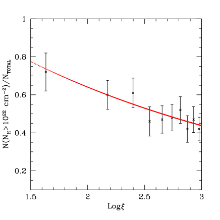
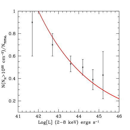
Figure 4: Upper panel: The simulation results for the fraction of obscured AGN as a function of the ionisation parameter (points) together with the best fit power-law model, F$\sim\xi^{-0.16}$ (solid line). Lower panel: The fraction of the obscured AGN as a function of luminosity in the combined XMM-Newton and Chandra data presented in Akylas et al. (2006) (points). The solid line represents the correlation predicted by our simulation model (F$\sim\L^{-0.16}$).

3 Discussion

3.1 The warm absorber

The results presented above demonstrate that the simplest photo-ionisation model can roughly reproduce the decrease in the fraction of obscured AGN at high luminosities. If this model is true it would imply that many luminous QSOs would present evidence for warm absorption. The absorption edges due to OVII and OVIII at 0.74 and 0.87 keV respectively are the strongest signatures of ionised gas at X-ray wavelengths. The high resolution achievable with the grating spectrometers on-board XMM-Newton and Chandra revealed many more absorption features as e.g. the Unresolved Transitional Array between 0.73 and 0.77 keV (Behar, Sako & Kahn 2001). These features are blue-shifted and show distinct velocity components (eg. Kaastra et al. 2000). This strongly suggests that the warm absorbers are associated with outflows. XMM-Newton high sensitivity spectroscopy with RGS (Guainazzi & Bianchi 2006) places tight constrains on the location of the warm absorber. These appear to be associated with the molecular torus. Warm absorbers are found in about 50% of nearby Seyfert galaxies (Reynolds 1997; Crenshaw, Kraemer & George 2003).

The picture was unclear at high (QSO) luminosities. are red-shifted at low energies. In the ASCA QSO samples of Reeves & Turner (2000) and George et al. (2000) there is little evidence for ionised absorption. Because of its high effective area, XMM-Newton routinely produced high signal-to-noise spectra and changed drastically the above picture. Piconcelli et al. (2005) find that about 50% of the 40 QSOs in their PG sample present warm absorbers.

It is interesting to investigate whether there is any evidence for the presence of warm absorber features in the spectra of luminous AGN in deep surveys. Here we examine the luminous AGN in the combined sample of Akylas et al. (2006). There are about 30 QSOs with $L_{X}>10^{44}$ $\rm erg\leavevmode\nobreak\ s^{-1}$ below a redshift of $\sim$1.2 where the oxygen absorption edges should be readily detected. Of these only 10 have a good signal-to-noise ratio with over 200 photons in their spectra. We fit a warm absorber model and find that 3 sources have an equally good fit with an ionised $\xi>100$ warm absorber, as compared to the cold absorber. Obviously the limited photon statistics do not allow for a conclusive test in this case.

3.2 The X-ray Baldwin effect

The Fe lines above 6 keV provide a census of the state of circumnuclear material in AGN. It is therefore reasonable to expect a relation between the obscuration fraction and the strength of the Fe lines. Iwasawa & Taniguchi (1993) first find that the equivalent width (EW) of the narrow Fe K$\alpha$ at 6.4 keV line decreases with the 2-10 keV X-ray luminosity in a sample of Seyfert galaxies observed by Ginga (the so called Iwasawa-Taniguchi or X-ray Baldwin effect). The correlations above closely resemble the well known Baldwin effect where the EW of the CIV 1550 Å line decreases with increasing optical luminosity (Baldwin 1977). The optical Baldwin effect has been corroborated by the results of Kinney et al. (1990) and more recently Croom et al. (2002) using 2dF data. The last authors find a relation with a slope of -0.128 $\pm$ 0.015. The Baldwin effect can be explained on the basis of either a diminishing covering factor or alternatively an increasing ionisation parameter (Mushotzky & Ferland 1984) with increasing luminosity.

Page et al. (2004) again find evidence for an X-ray Baldwin effect using Seyfert and QSO data that span more than 5 orders of magnitude in luminosity. They find a correlation between the narrow core of the Fe K_α EW and the 2-10 keV X-ray luminosity in the form of $EW\propto L_{X}^{-0.17\pm 0.08}$. More specifically, the EW obtains values around 150 eV at low luminosities ($\rm L_{X}(2-10keV)<10^{43}$ $\rm erg\leavevmode\nobreak\ s^{-1}$), dropping to less than 50 eV at high luminosities ($L_{X}>10^{46}$ $\rm erg\leavevmode\nobreak\ s^{-1}$). Jiang et al. (2006) confirmed the X-ray Baldwin effect using Chandra data. Recent results by Bianchi et al. (2007) shed more light to the above issues. They find a highly significant anti-correlation of narrow Fe K_α line EW with respect to the Eddington ratio while no dependence on the black hole mass is apparent. Moreover they find a correlation between the ratio of highly ionised to neutral FeK line flux with luminosity that supports our photo-ionisation scenario. Note however that according to their claims this is a rather weak result ($\rm Log(R)=(0.12\pm 0.06)+(0.09\pm 0.06)Log(L_{X_{44}}$) to explain the observed X-ray Baldwin effect.

It is interesting to note that the X-ray Baldwin effect is also present in the broad component of the FeK line. Nandra et al. (1997) find an anti-correlation of the broad Fe line EW with the 2-10 keV luminosity in a sample of 18 Seyfert galaxies observed by ASCA. The broad FeK line most likely originates in the accretion disk. Nandra et al. (1997) assert that the most obvious explanation for the X-ray Baldwin effect observed is the photo-ionisation of the accretion disk.

4 Conclusions

We employ X-ray spectral simulations to determine the effect of photo-ionisation on the obscuring torus in AGN. In particular, our goal is to explore whether photo-ionisation can explain the steep decrease in the fraction of obscured AGN with increasing luminosity as witnessed in X-ray surveys. Our conclusions can be summarised as follows:

• Photo-ionisation can reproduce the observed decrease in the absorbed AGN fraction as a function of luminosity. We find that the fraction of absorbed AGN should fall with luminosity as $L^{-0.16\pm 0.03}$ in rough agreement with the observations.

• The observed decrease in the obscuring material covering factor is roughly consistent with the dependence of the Fe K_α line equivalent width on luminosity, the X-ray Baldwin effect.

• A simple prediction of the photo-ionised model is that a high fraction of luminous QSOs should present warm absorption features in their X-ray spectra. Future, high effective area mission, such as XEUS will be able to quantitatively assess this scenario.

References

- (1) Akylas, A., Georgantopoulos, I., Georgakakis, A., Kitsionas, S., Hatziminaoglou, E., 2006, A&A, 459, 693
- (2) Alexander, D. M., Bauer, F. E., Brandt, W. N., et al. 2003, AJ, 126, 539
- (3) Arnaud, K. A., 1996, ASPC, 101, 17
- (4) Baldwin, J. A., 1977, ApJ, 214, 679
- (5) Behar, E., Sako, M., Kahn, S. M., 2001, ApJ, 563, 497
- (6) Bianchi, S., Guainazzi, M., Matt, G., Fonseca Bonilla, N., 2007, A&A, 467, 19
- (7) Caccianiga, A., Severgnini, P., Braito, V., et al. 2004, A&A, 416, 901
- (8) Cash, W., 1979, ApJ, 228, 939
- (9) Comastri, A., Setti, G. Zamorani, G., & Hasinger, G. 1995, A&A, 296, 1
- (10) Comastri, A., Fiore, F., Vignali, C., Matt, G., Perola, G. C., La Franca, F., 2001, MNRAS, 327, 781
- (11) Crenshaw, D. M., Kraemer, S. B., & George, I. M., 2003, ARA&A
- (12) Croom, S. M., Rhook, K., Corbett, E. A., Boyle, B. J., et al. 2002, MNRAS, 337, 275
- (13) Done, C., Mulchaey, J. S., Mushotzky, R. F., Arnaud, K. A., 1992, ApJ, 395, 275
- (14) Georgantopoulos, I., Georgakakis, A., Akylas, A., Stewart, G. C., Giannakis, O., Shanks, T., Kitsionas, S., 2004, MNRAS, 352, 91
- (15) George, I. M., Turner, T. J., Yaqoob, T., Netzer, H., Laor, A., Mushotzky, R. F., Nandra, K., Takahashi, T., 2000 ApJ, 531, 52
- (16) Giacconi, R., Zirm, A., Wang, J. et al. 2002, ApJS, 139, 369
- (17) Gilli, R., Comastri, A., Hasinger, G, 2007, A&A, 463, 79
- (18) Guainazzi, M., Bianchi, S., 2006, astro.ph/0612488
- (19) Iwasawa, K., Taniguchi, Y., 1993, ApJ, 413, 15L
- (20) Jaffe, W., Meisenheimer, K., Röttgering, H. J. A., 2004, Nature, 429, 47
- (21) Jiang, P., Wang, J. X., Wang, T. G., 2006, ApJ, 644, 725
- (22) Kaastra, J. S., Mewe, R., Liedahl, D. A., Komossa, S., Brinkman, A. C., 2000, A&A, 354, 83L
- (23) Kinney, A. L., Rivolo, A. R., Koratkar, A. P., 1990, ApJ, 357, 338
- (24) Köningl, A. & Kartje, J.F., 1994, ApJ, 434, 446
- (25) Lawrence, A., 1991, MNRAS, 252, 586L
- (26) La Franca, F., Fiore, F., Comastri, A., et al. 2005, AJ, 635, 864
- (27) Mushotzky, R. F., & Ferland, G. J., 1984, ApJ, 278, 558
- (28) Nandra, K., & Pounds, K. A., 1994, MNRAS, 268, 405
- (29) Nandra, K., George, I. M., Mushotzky, R. F., Turner, T. J., Yaqoob, T., 1997, ApJ, 488, 91
- (30) Page, K. L., O’Brien, P. T., Reeves, J. N., Turner, M. J. L., 2004, MNRAS, 347, 316
- (31) Perola, G. C., Puccetti, S., Fiore, F., et al. 2004, A&A, 421, 491
- (32) Peterson, B. M., 2006, LNP, 693, 77
- (33) Piconcelli, E., Cappi, M., Bassani, L., Fiore, F., Di Cocco, G., Stephen, J. B. 2002, A&A, 394, 835
- (34) Piconcelli, E.; Jimenez-Bailn, E., Guainazzi, M., Schartel, N., Rodriguez-Pascual, P. M., Santos-Lle, M., 2005, A&A, 432, 15
- (35) Prieto, M. A., Meisenheimer, K.,Marco, O., 2004, ApJ, 614, 135
- (36) Reeves, J. N., Turner, M. J. L., 2000, MNRAS, 316, 234
- (37) Reynolds, C. S., 1997, MNRAS, 286, 513
- (38) Risaliti, G., Elvis, M., Nicastro, F.,2002, ApJ, 571, 234
- (39) Simpson, C. 2005, MNRAS, 360, 565
- (40) Steffen, A. T., Barger, A. J., Cowie, L. L., Mushotzky, R. F., Yang, Y., 2003, ApJ, 596, 23
- (41) Tozzi, P., Gilli, R., Mainieri, V., et al. 2006, A&A, 451, 457
- (42) Ueda, Y., Akiyama, M., Ohta, K., & Miyaji, T. 2003, ApJ, 598, 886