Microlensing of the X-ray, UV and optical emission regions of quasars: Simulations of the time-scales and amplitude variations of microlensing events

Abstract

We consider the influence of microlensing on different spectral bands of lensed QSOs. We assumed that the emitting X-ray, UV and optical regions are different in size, but that the continuum emission in these spectral bands is originating from an accretion disc. Estimations of the time scales for microlensing and flux amplification in different bands are given. We found that the microlensing duration should be shorter in the X-ray (several months) than in UV/optical emitting region (several years). This result indicates that monitoring of the X-ray variations in lensed QSOs that show a ’flux anomaly’ can clarify the source of this anomaly.

1 Introduction

Recent observational and theoretical studies suggest that gravitational microlensing can induce variability not only in optical light, but also in the X-ray emission of lensed QSOs (Chartas et al., 2002, 2004; Dai et al., 2003, 2004; Jovanović, 2006; Popović et al., 2001, 2003a, 2003b, 2006a, 2006b). Variability studies of QSOs indicate that the size of the X-ray emitting region is significantly smaller ($\sim$ several light hours), than the optical and UV emitting regions ($\sim$ several light days).

Gravitational lensing is achromatic (the deflection angle of a light ray does not depend on its wavelength), but it is clear that if the geometries of the emitting regions at different wavelengths are different then chromatic effects could occur. For example, if the microlens is a binary star or if the microlensed source is extended (Griest & Hu, 1992, 1993; Bogdanov and Cherepashchuk, 1995a, b; Zakharov, 1997; Zakharov & Sazhin, 1998; Popović & Chartas, 2005) different amplifications in different spectral bands can be present. Studies aiming to determine the influence of microlensing on the spectra of lensed QSOs need to take into account the complex structure of the QSO central emitting region (Popović & Chartas, 2005). Since the sizes of the emitting regions are wavelength dependent, microlensing by stars in the lens galaxy may lead to a wavelength dependent magnification. For example, Blackburne et al. (2006) reported such a ’flux anomaly’ in quadruply imaged quasar 1RXS J1131-1231. In particular, they found discrepancies between the X-ray and optical flux ratio anomalies. Such anomalies in the different spectral band flux ratios can be attributed to micro- or milli-lensing in the massive lensing halo. In the case of milli-lensing one can infer the nature of substructure in the lensing galaxy, which can be connected to Cold Dark Matter (CDM) structures (see e.g. Dobler & Keeton 2006). Besides microlensing, there are several mechanisms which can produce flux anomalies, such as extinction and intrinsic variability. These anomalies were discussed in Popović & Chartas (2005) where the authors gave a method that can aid in distinguishing between variations produced by microlensing from ones resulting from other effects. In this paper we discuss consequences of variations due to gravitational microlensing, in which the different geometries and dimensions of emitting regions of different spectral bands are considered.

The influence of microlensing on QSO spectra emitted from their accretion discs in the range from the X-ray to the optical spectral band is analyzed. Moreover, assuming different sizes of the emitting regions, we investigate the microlensing time scales for those regions, as well as a time dependent response in amplification of different spectral bands due to microlensing. Also, we give the estimates of microlensing time scales for a sample of lensed QSOs.

In Section 2, we describe our model of the quasar emitting regions and a model of the micro-lens. In Section 3 we discuss the time scales of microlensing and in Section 4 we present our results. Finally, in Section 5, we draw our conclusions.

2 A model of QSO emitting regions and microlens

2.1 A model of the QSO emitting regions

In our models we adopt a disc geometry for the emitting regions of Active Galactic Nuclei (AGN) since the most widely accepted paradigm for AGN includes a supermassive black hole fed by an accretion disc. Fabian et al. (1989) calculated spectral line profiles for radiation emitted from the inner parts of accretion discs and later on such features of Fe $K\alpha$ lines were discovered by Tanaka et al. (1995) in Japanese ASCA satellite data for Seyfert galaxy MGC-6-30-15. Moreover, the assumption of a disc geometry for the distribution of the emitters in the central part is supported by the spectral shape of the Fe K$\alpha$ line in AGN (e.g. Nandra et al. (1997), see also results of simulations (Zakharov & Repin, 1999, 2002; Zakharov et al., 2003; Zakharov & Repin, 2003a, b, c, 2004; Zakharov & Repin, 2005, 2006; Zakharov, 2004, 2007)). On the other hand, very often a bump in the UV band is present in the spectra of AGN, that indicates that the UV and optical continuum originates in an accretion disk.

We should note here that probably most of the X-ray emission in the 1–10 keV energy range originates from inverse Compton scattering of photons from the disc by electrons in a tenuous hot corona. Proposed geometries of the hot corona of AGN include a spherical corona sandwiching the disc and a patchy corona made of a few compact regions covering a small fraction of the disc (see e.g. Malzac (2007)). On the other hand, it is known that part of the accretion disc that emits in the 1–10 keV rest-frame band (e.g. the region that emits the continuum Compton reflection component and the fluorescent emission lines) is very compact and may contribute to X-ray variability in this energy range. In order to study the microlensing time scales, one should consider the dimensions of the X-ray emitting region which are very important for the integral flux variations due to microlensing. The geometry of the emitting regions adopted in microlensing models will affect the simulated spectra of the continuum and spectral line emission (Popović & Chartas, 2005; Jovanović, 2006). In this paper we assume that the AGN emission from the optical to the X-ray band originates from different parts of the accretion disc.

Also we assume that we have a stratification in the disc, where the innermost part emits the X-ray radiation and outer parts the UV and optical continuum emission. To study the effects of microlensing on a compact accretion disc we use the ray-tracing method, considering only those photon trajectories that reach the sky plane at a given observer angle (see, e.g. Popović et al. 2003a,b and references therein). The amplified brightness with amplification $A(X,Y)$ for the continuum is given by

$$I_{C}(X,Y;E_{obs})={{I_{P}}}(E_{obs},T(X,Y))\cdot A(X,Y),$$ (1)

where $T(X,Y)$ is the temperature, $X$ and $Y$ are the impact parameters which describe the apparent position of each point of the accretion disc image on the celestial sphere as seen by an observer at infinity, $E_{\rm obs}$ is the observed energy, $I_{P}$ is an emissivity function.

In the standard Shakura-Sunyaev disc model (1973), accretion occurs via an optically thick and geometrically thin disc. The effective optical depth in the disc is very high and photons are close to the thermal equilibrium with electrons. The surface temperature is a function of disc parameters and results in the multicolor black body spectrum. This component is thought to explain the ’blue bump’ in AGN and the soft X-ray emission in galactic black holes. Although the standard Shakura-Sunyaev disc model does not predict the power-law X-ray emission observed in all sub-Eddington accreting black holes, the power law for the X-ray emissivity in AGN is usually adopted (see e.g. Nandra et al. (1999)). But one can not exclude other approximations for emissivity laws, such as black-body or modified black-body emissivity laws. Moreover, we will assume that the emissivity law is the same through the whole disc. Therefore we used the black-body radiation law. The disc emissivity is given as (e.g. Jaroszynski (1992)):

$$I_{P}(X,Y;E)=B[E,T_{s}(X,Y)],$$

where

$$B\left({E,T_{s}(X,Y)}\right)={\frac{{2E^{3}}}{{h^{2}c^{2}}}}{\frac{{1}}{{e^{{{E}\mathord{\left/{\vphantom{{h\nu}{kT}}}\right.\kern-1.2pt}{kT_{s}(X,Y)}}}-1}}},$$ (2)

where $c$ is the speed of light, $h$ is the Planck constant, $k$ is the Boltzmann constant and $T_{s}(X,Y)$ is the surface temperature. Concerning the standard accretion disc (Shakura & Sunayev, 1973), here we assumed that (see Popović et al. (2006a)):

$$T_{s}(X,Y)\sim r^{-3/2}(X,Y)(1-r^{-1/2}(X,Y))^{4/5}\,{\rm K},$$ (3)

taking that an effective temperature in the innermost part (where X-ray is originated) is in an interval from 10⁷ K to 10⁸ K.

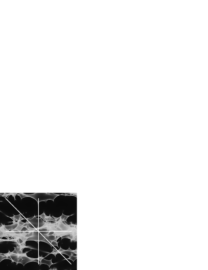
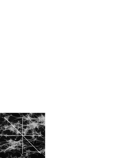
Figure 1: Magnification map of the QSO 2237+0305A image (left) and of a ”typical” lens system (right). The white solid lines represent three analyzed paths of an accretion disc center: horizontal ($y=0$), diagonal ($y=-x$) and vertical ($x=0$).

2.2 A model for microlensing

To explain the observed microlensing events in quasars, one can use different microlensing models. The simplest approximation is a point-like microlens, where microlensing is caused by some compact isolated object (e.g. by a star). Such a microlens is characterized by its Einstein Ring Radius in the lens plane: $ERR=\sqrt{\dfrac{4Gm}{c^{2}}\dfrac{D_{l}D_{ls}}{D_{s}}}$ or by the corresponding projection in the source plane: $R_{E}=\dfrac{D_{s}}{D_{l}}ERR=\sqrt{\dfrac{4Gm}{c^{2}}\dfrac{D_{s}D_{ls}}{D_{l}}}$, where $G$ is the gravitational constant, $c$ is the speed of light, $m$ is the microlens mass and $D_{l}$, $D_{s}$ and $D_{ls}$ are the cosmological angular distances between observer-lens, observer-source and lens-source, respectively. In most cases we can not simply consider that microlensing is caused by an isolated compact object but we must take into account that the micro-deflector is located in an extended object (typically, the lens galaxy). Therefore, when the size of the Einstein ring radius projection $R_{E}$ of the microlens is larger than the size of the accretion disc and when a number of microlenses form a caustic net, one can describe the microlensing in terms of the crossing of the disc by a straight fold caustic (Schneider et al. 1992). The amplification at a point of an extended source (accretion disc) close to the caustic is given by Chang & Refsdal (1984) (a more general expression for a magnification near a cusp type singularity is given by Schneider & Weiss (1992); Zakharov (1995)):

$$A(X,Y)=A_{0}+K\sqrt{\frac{r_{\rm caustic}}{\kappa(\xi-\xi_{c})}}\cdot H(\kappa(\xi-\xi_{c})),$$ (4)

where $A_{0}$ is the amplification outside the caustic and $K=A_{0}\beta$ is the caustic amplification factor, where $\beta$ is constant of order of unity (e.g. Witt et al. 1993). The ”caustic size” $r_{\rm caustic}$ is the distance in a direction perpendicular to the caustic for which the caustic amplification is 1, and therefore this parameter defines a typical linear scale for the caustic in the direction perpendicular to the caustic. $\xi$ is the distance perpendicular to the caustic in gravitational radii units and $\xi_{c}$ is the minimum distance from the disc center to the caustic. Thus,

$$\xi_{c}={\sqrt{X_{c}^{2}+Y_{c}^{2}}},$$ (5)

$${\rm tg}\alpha=\frac{Y_{c}}{X_{c}},$$ (6)

and

$$\xi=\xi_{c}+\frac{(X-X_{c}){\rm tg}\phi+Y_{c}-Y}{\sqrt{{\rm tg}^{2}\phi+1}},$$ (7)

where $\phi=\alpha+{\pi/2}$. $H(\kappa(\xi-\xi_{c}))$ is the Heaviside function, $H(\kappa(\xi-\xi_{c}))=1$, for $\kappa(\xi-\xi_{c})>0$, otherwise it is 0. $\kappa$ is $\pm 1$, it depends on the direction of caustic motion; if the direction of the caustic motion is from approaching side of the disc $\kappa=-1$, otherwise it is +1. Also, in the special case of caustic crossing perpendicular to the rotating axis $\kappa=+1$ for direction of caustic motion from $-Y$ to $+Y$, otherwise it is $-1$. A microlensing event where a caustic crosses over an emission region can be described in the following way: before the caustic reaches the emission region, the amplification is equal to $A_{0}$ because the Heavisied function of equation (4) is zero. Just as the caustic begins to cross the emitting region the amplification rises rapidly and then decays gradually towards $A_{0}$ as the source moves away from the caustic-fold.

Moreover, for the specific event one can model the caustic shape to obtain different parameters (see e.g. Abajas et al. 2005, Kochanek 2004 for the case of Q2237+0305). In order to apply an appropriate microlens model, additionally we will consider a standard microlensing magnification pattern for the Q2237+0305A image (Fig. 1 left). For generating this map we used the ray-shooting method (Kayser et al., 1986; Schneider & Weiss, 1986, 1987; Wambsganss et al., 1990a, b). In this method the input parameters are the average surface mass density $\sigma$, shear $\gamma$ and width of the microlensing magnification map expressed in units of the Einstein ring radius (defined for one solar mass in the lens plane).

First, we generate a random star field in the lens plane with use of the parameter $\sigma$. After that, we solve the Poisson equation $\nabla^{2}\psi=2\sigma$ in the lens plane numerically, so we can determine the lens potential $\psi$ in every point of the grid in the lens plane. To solve the Poisson equation numerically one has to write its finite difference form:

$$\psi_{i+1,j}+\psi_{i-1,j}+\psi_{i,j+1}+\psi_{i,j-1}-4\psi_{i,j}=2\sigma_{i,j}.$$ (8)

Here we used the standard 5-point formula for the two-dimensional Laplacian. Next step is inversion of the equation (8) using Fourier transform. After some transformations we obtain:

$$\hat{\psi}=\frac{\hat{\sigma}_{mn}}{2(\cos{\frac{m\pi}{N_{1}}}+\cos{\frac{n\pi}{N_{2}}}-2)},$$ (9)

where $N_{1}$ and $N_{2}$ are dimensions of the grid in the lens plane. Now, using the finite difference technique, we can compute the deflection angle $\vec{\alpha}=\nabla\psi$ in each point of the grid in the lens plane. After computing deflection angle, we can map the regular grid of points in the lens plane, via lens equation, onto the source plane. These light rays are then collected in pixels in the source plane, and the number of rays in one pixel is proportional to the magnification due to microlensing at this point in the source plane.

Typically, for calculations of microlensing in gravitationally lensed systems one can consider cases where dimensionless surface mass density $\sigma$ is some fraction of 1 e.g. 0.2, 0.4, 0.6, 0.8 (Treyer & Wambsganss, 2004), cases without external shear ($\gamma=0$) and cases with $\gamma=\sigma$ for isothermal sphere model for the lensing galaxy. In this article we assume the values of these parameters within the range generally adopted by other authors, in particular by Treyer & Wambsganss (2004).

Microlensing magnification pattern for the Q2237+0305A image (Fig. 1 left) with 16 $R_{E}$ on a side (where $R_{E}\approx 5867\ R_{g}$) is calculated using the following parameters: $\sigma=0.36$ and $\gamma=0.4$ (see Popović et al. (2006a), Fig. 2), the mass of microlens is taken to be 0.3$M_{\odot}$ and we assume a flat cosmological model with $\Omega=0.3$ and $H_{0}=75\ \rm km\ s^{-1}Mpc^{-1}$.

We also calculated microlensing magnification pattern for a ”typical” lens system (Fig. 1 right), where the redshifts of microlens and source are: $z_{l}=0.5$ and $z_{s}=2$. In this case, the microlens parameters are taken arbitrary: $\sigma=0.45$ and $\gamma=0.3$ and the size of obtained microlensing pattern is also $16\ R_{E}\times 16\ R_{E}$, where $R_{E}\approx 3107\ R_{g}$.

3 Typical time scales for microlensing

Typical scales for microlensing are discussed not only in books on gravitational lensing (Schneider, Ehlers & Falco, 1992; Zakharov, 1997; Petters, Levine & Wambsganss, 2001), but in recent papers also (see, for example, Treyer & Wambsganss (2004)). In this paper we discuss microlenses located in gravitational macrolenses (stars in lensing galaxies), since optical depth for microlensing is then the highest (Wyithe & Turner, 2002a; Wyithe & Turner, 2002b; Zakharov, Popović & Jovanović, 2004, 2005) in comparison with other possible locations of gravitational microlenses, as for example stars situated in galactic clusters and extragalactic dark halos (Tadros, Warren & Hewett, 1998; Totani, 2003; Inoue & Chiba, 2003).

Assuming the concordance cosmological model with $\Omega_{\rm tot}=1$, $\Omega_{\rm matter}=0.3$ and $\Omega_{\Lambda}=0.7$ we recall that typical length scale for microlensing is (Treyer & Wambsganss, 2004):

$$R_{E}=\sqrt{2r_{s}\cdot\frac{D_{s}D_{ls}}{D_{l}}}\approx 3.2\cdot 10^{16}\sqrt{\frac{m}{M_{\odot}}}h_{75}^{-0.5}\mathrm{~{}cm},$$ (10)

where ”typical” microlens and sources redshifts are assumed to be $z_{l}=0.5,z_{s}=2.$ (similar to Treyer & Wambsganss (2004)), $r_{s}=\dfrac{2Gm}{c^{2}}$ is the Schwarzschild radius corresponding to microlens mass $m$, $h_{75}=H_{0}/((75{\rm~{}km/sec})/{\rm Mpc})$ is dimensionless Hubble constant.

The corresponding angular scale is (Treyer & Wambsganss, 2004)

$$\theta_{0}=\frac{R_{E}}{D_{s}}\approx 2.2\cdot 10^{-6}\sqrt{\frac{m}{M_{\odot}}}h_{75}^{-0.5}{\rm~{}arcsec},$$ (11)

Using the length scale (10) and velocity scale (say $v_{\bot}\sim$ 600 km/sec as Treyer & Wambsganss (2004) did), one could calculate the standard time scale corresponding to the scale to cross the projected Einstein radius

$$t_{E}=(1+z_{l})\frac{R_{E}}{v_{\bot}}\approx 25\sqrt{\frac{m}{M_{\odot}}}v_{600}^{-1}h_{75}^{-0.5}{\rm~{}years},$$ (12)

where a relative transverse velocity $v_{600}=v_{\bot}/(600$ km/sec). The time scale $t_{E}$, corresponding to a point-mass lens and to a small source (compared to the projected Einstein radius of the lens), could be used if microlenses are distributed freely at cosmological distances and if each Einstein angle is located far enough from another one. However, the estimation (12) gives long and most likely overestimated time scales especially for gravitationally lensed systems. Thus we must apply another microlens model to estimate time scales.

For a simple caustic model, such as one that considers a straight fold caustic, there are two time scales depending either on the ”caustic size” ($r_{\rm caustic}$) or the source radius ($R_{\rm source}$). In the case when source radius is larger or at least close to the ”caustic size” ($R_{\rm source}\gtrsim r_{\rm caustic}$), the relevant time scale is the ”crossing time” (Treyer & Wambsganss, 2004):

$$t_{\rm cross} = (1+z_{l})\frac{R_{\rm source}}{v_{\bot}(D_{s}/D_{l})}$$

$$\approx 0.69\ R_{15}\ v_{600}^{-1}\left(\frac{D_{s}}{D_{l}}\right)^{-1}h_{75}^{-0.5}{\rm~{}years}$$

$$\approx 251\ R_{15}\ v_{600}^{-1}\ h_{75}^{-0.5}{\rm~{}days},$$

where $D_{l}$ and $D_{s}$ correspond to $z_{l}=0.5$ and $z_{s}=2$, respectively and $R_{15}=R_{\rm source}/10^{15}$ cm. As a matter of fact, the velocity perpendicular to the straight fold caustic characterizes the time scale and it is equal to $v_{\bot}\sin\beta$ where $\beta$ is the angle between the caustic and the velocity $v_{\bot}$ in the lens plane, but in our rough estimates we can omit factor $\sin\beta$ which is about unity. However, if the source radius $R_{\rm source}$ is much smaller than the ”caustic size” $r_{\rm caustic}$ ($R_{\rm source}\ll r_{\rm caustic}$), one could use the ”caustic time”, i.e. the time when the source is located in the area near the caustic:

$$t_{\rm caustic} = (1+z_{l})\frac{r_{\rm caustic}}{v_{\bot}(D_{s}/D_{l})}$$

$$\approx 0.69\ r_{15}\ v_{600}^{-1}\left(\frac{D_{s}}{D_{l}}\right)^{-1}h_{75}^{-0.5}{\rm~{}years}$$

$$\approx 251\ r_{15}\ v_{600}^{-1}\ h_{75}^{-0.5}{\rm~{}days},$$

where $r_{15}=r_{\rm caustic}/10^{15}$ cm.

Therefore, $t_{\rm cross}$ could be used as a lower limit for typical time scales in the case of a simple caustic microlens model. From equations (3) and (3) it is clear that one cannot unambiguously infer the source size $R_{\rm source}$ from variability measurements alone, without making some further assumptions. In general, however, we expect that $t_{\rm cross}$ corresponds to smaller amplitude variations than $t_{\rm caustic}$, since in the first case only a fraction of a source is significantly amplified by a caustic (due to assumption that $R_{\rm source}\gtrsim r_{\rm caustic}$), while in the second case it is likely that the entire source could be strongly affected by caustic amplification (due to assumption that $R_{\rm source}\ll r_{\rm caustic}$).

Figure 2: The variations of normalized total continuum flux in optical (3500–7000 Å), UV (1000–3500 Å) and X (1.24–12.4 Å i.e. 1–10 KeV) band due to microlensing by a caustic crossing along $y=-x$ direction in the case of Schwarzschild metric. Time scale corresponds to ”typical” redshifts of microlens and source: $z_{l}=0.5$ and $z_{s}=2$. The parameters of the caustic are: $A_{0}$=1, $\beta$=1, $\kappa=+1$ and its ”size” is 9000 $R_{g}$. Negative distances and times correspond to the approaching side, and positive to the receding side of accretion disc. In this case, due to $\kappa=+1$, caustic motion is from the receding towards the approaching side (i.e. from the right to the left). The source mass is $10^{8}\ M_{\odot}$. The radii of optical emitting region are: $R_{in}=100\ R_{g}$, $R_{out}=2000\ R_{g}$, for UV emitting region: $R_{in}=100\ R_{g}$, $R_{out}=1000\ R_{g}$ and for X emitting region: $R_{in}=R_{ms}$, $R_{out}=80\ R_{g}$.

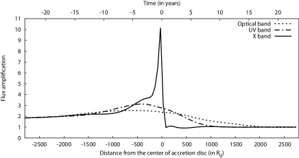
Figure 3: The same as in Fig. 2. but for $r_{\rm caustic}=2000\ R_{g}$.

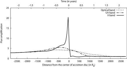
Figure 4: The same as in Fig. 2. in the case when time scale corresponds to $z_{l}=0.04$, $z_{s}=1.69$ (i.e. to Q2237+0305 lens system).

In this paper, we estimated the microlensing time scales for the X-ray, UV and optical emitting regions of the accretion disc using the following three methods:

1. by converting the distance scales of microlensing events to the corresponding time scales according to the formula (13) in which $R_{\rm source}$ is replaced by the distance from the center of accretion disc. Caustic rise times ($t_{HME}$) are then derived from the simulated variations of the normalized total flux in the X-ray, UV and optical spectral bands (see Figs. 2-4) by measuring the time from the beginning to the peak of the magnification event

2. by calculating the caustic times ($t_{\rm caustic}$) according to equation (14)

3. using light curves (see Figs. 5 and 6) produced when the source crosses over a magnification pattern. Rise times of high magnification events ($t_{HME}$) are then measured as the time intervals between the beginning and the maximum of the corresponding microlensing events (for more details, see the next section).

4 Results and discussion

In order to explore different cases of microlensing and evaluate time scales for different spectral bands, first we numerically simulate the crossing of a straight-fold caustic with parameters $A_{0}=1,\ \beta=1$, $\kappa=+1$ and $r_{\rm caustic}=9000$ $R_{g}$ over an accretion disc with an inclination angle 35^∘, that is stratified into three parts:

(i) The innermost part that emits X-ray continuum (1.24 Å – 12.4 Å or 1–10 keV). The inner radius is taken to be $R_{inn}=R_{ms}$ (where $R_{ms}$ is the radius of the marginally stable orbit: $R_{ms}=6\ R_{g}$ in the Schwarzschild metric) and outer radius is $R_{out}=80$ $R_{g}$ (where $R_{g}=GM/c^{2}$ is the gravitational radius for a black hole with mass $M$).

(ii) An UV emitting part of the disc (contribute to the emission from 1000 Å – 3500Å), with $R_{inn}=100$ $R_{g}$ and $R_{out}=1000$ $R_{g}$.

(iii) An outer optical part of the disc with $R_{inn}=100$ $R_{g}$ and $R_{out}=2000$ $R_{g}$ that emits in the wavelength band from 3500 Å until 7000 Å.

Table 1: The estimated time scales (in years) for microlensing of the X-ray, UV and optical emission region for lensed QSOs observed by Chandra X-ray Observatory (Dai et al., 2004). The calculated caustic times $t_{\rm caustic}$ are obtained according to formula (14) for the following values of the cosmological constants: $H_{0}=75\rm\ km\ s^{-1}Mpc^{-1}$ and $\Omega_{0}=0.3$. The caustic rise times $t_{HME}$ are derived from caustic crossing simulations (see Figs 2 – 4). The black hole mass is assumed to be 10${}^{8}\rm M_{\odot}$.

Object	$z_{s}$	$z_{l}$	X-ray		UV		optical
			$t_{\rm caustic}$	$t_{HME}$	$t_{\rm caustic}$	$t_{HME}$	$t_{\rm caustic}$	$t_{HME}$
HS 0818+1227	3.115	0.39	0.572	0.660	7.147	7.070	14.293	15.160
RXJ 0911.4+0551	2.800	0.77	0.976	1.120	12.200	12.080	24.399	25.880
LBQS 1009-0252	2.740	0.88	1.077	1.240	13.468	13.330	26.935	28.570
HE 1104-1805	2.303	0.73	0.918	1.050	11.479	11.370	22.957	24.350
PG 1115+080	1.720	0.31	0.451	0.520	5.634	5.570	11.269	11.950
HE 2149-2745	2.033	0.50	0.675	0.780	8.436	8.350	16.871	17.890
Q 2237+0305	1.695	0.04	0.066	0.080	0.828	0.820	1.655	1.760

Table 2: Average rise times ($<t_{HME}>$) of high magnification events, their average number ($<N_{\rm caustic}>_{0}$) per unit length ($R_{E}$) and their average number ($<N_{\rm caustic}>_{y}$) per year in the light curves of Q2237+0305A (Fig. 5) and ”typical” lens system (Fig. 6).

		Q2237+0305			”Typical” lens
Disc path	Sp. band	$<t_{HME}>$	$<N_{\rm caustic}>_{0}$	$<N_{\rm caustic}>_{y}$	$<t_{HME}>$	$<N_{\rm caustic}>_{0}$	$<N_{\rm caustic}>_{y}$
	X	0.37	0.95	0.20	3.94	1.63	0.06
$y=0$	UV	1.29	0.59	0.12	10.96	0.78	0.03
	Optical	2.96	0.51	0.10	15.81	0.62	0.02
	X	0.57	0.52	0.11	2.77	1.65	0.06
$y=-x$	UV	1.92	0.36	0.07	6.62	0.49	0.02
	Optical	3.98	0.26	0.05	17.04	0.38	0.01
	X	0.68	1.61	0.33	4.52	1.40	0.05
$x=0$	UV	1.38	0.88	0.18	13.25	0.54	0.02
	Optical	2.96	0.44	0.09	31.62	0.31	0.01

Having in mind that the aims of this investigation are to study the microlensing time scales for different emitting regions and time dependent response of amplification in different spectral bands, we considered microlensing magnification patterns only for image A of Q2237+0305 and for a ”typical” lens system. Our intention was not to create a complete microlensing model for a specific lens system, and therefore we did not analyze the differences between images (as for instance the time delay between them). The variations in the total flux in the different spectral bands are given in Figs. 2–6. In Figs. 2 and 3 the simulations for a typical lens system with $z_{l}=0.5$ and $z_{s}=2$ and for two different ”caustic sizes” are given. As one can see from Figs. 2 and 3, the microlensing time scales are different for different regions, and the durations of variations in the X-ray are on order of several months to a few years, but in the UV/optical emission regions they are on order of several years. Also, as one can see in Figs. 2 and 3, the time scales do not depend on ”caustic size” which, on the other hand, affects only the maximal amplifications in all three spectral bands. The results corresponding to the lens system of QSO 2237+0305 ($z_{l}=0.04$, $z_{s}=1.69$) are given in Figs. 4 and 5. We considered the straight-fold caustic (Fig. 4) and a microlensing pattern for the image A of QSO 2237+0305 (Fig. 5). As one can see from Figs. 4 and 5, a higher amplification in the X-ray continuum than in the UV/optical is expected. In this case, the corresponding time scales are much shorter and they are from a few days up to a few months for X-ray and a few years for UV/optical spectral bands. The similar conclusion arises when we compare the latter results with those for a ”typical” lens system in the case of microlensing pattern (Fig. 6).

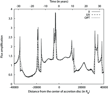
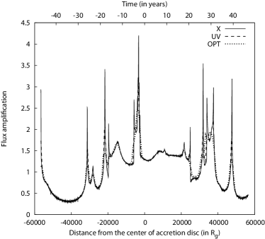
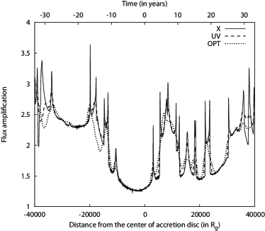
Figure 5: Variations in the X-ray (solid), UV (dashed) and optical (dotted) spectral bands corresponding to the horizontal (top left), diagonal (top right) and vertical (bottom) path in the magnification map of the QSO 2237+0305A (Fig. 1 left).

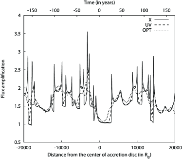
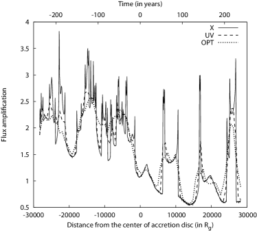
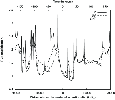
Figure 6: The same as in Fig. 5 but for the magnification map of a ”typical” lens system (Fig. 1 right).

We also estimated time scales for seven lensed QSOs which have been observed in the X-ray band (Dai et al., 2004). For each spectral band two estimates are made: caustic time ($t_{\rm caustic}$) - obtained from equation (14) and caustic rise time ($t_{HME}$) - obtained from caustic crossing simulations (see Figs. 2 – 4). In the second case, we measured the time from the beginning of the microlensing event until it reaches its maximum (i.e. in the direction from the right to the left in Figs. 2 – 4). The duration of the magnification event beyond the maximum of the amplification could not be accurately determined because of the asymptotic decrease of the magnification curve beyond the peak. Estimated time scales for different spectral bands are given in Table 1. As one can see from Table 1, the microlensing time scales are significantly smaller for the X-ray than for the UV/optical bands.

Unamplified and amplified brightness profiles of the X-ray emitting region, corresponding to the highest peak in Fig. 5 (top right) are presented in Fig. 7. As one can see in Fig. 7, the assumed brightness profile of the source is very complex due to applied ray tracing method, which allows us to obtain an image of the entire disc, not only its one dimensional profile. Therefore, we could not use a simple source profile for the calculation of microlensing time scales (as it was done by Witt et al. (1995)). Instead, we estimated the frequency of high amplification events (HMEs), i.e. the number of such events per unit length, directly from the light curves presented in Figs 5 and 6. For models with non-zero shear, this frequency depends on the direction of motion and for both calculated maps (Q2237+0305A and ”typical” lens) we counted the number of high magnification events along the following paths (see Fig. 1): i) horizontal ($y=0$) in the direction from $-x$ to $x$, ii) diagonal ($y=-x$) in direction from $-x$ to $x$ and iii) vertical ($x=0$) in direction from $y$ to $-y$. For each map the lengths of the horizontal and vertical paths in the source plane are the same (13.636 $R_{E}$ for Q2237+0305A and 12.875 $R_{E}$ for ”typical” lens), as well as are the corresponding crossing times (66.22 years for Q2237+0305A and 337.32 years for ”typical” lens). For Q2237+0305A the length of the diagonal path in source plane is 19.284 $R_{E}$ and the crossing time is 93.62 years, while the corresponding length in the ”typical” case is 18.208 $R_{E}$ and the crossing time is 477.04 years.

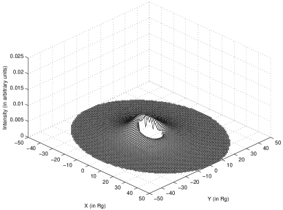
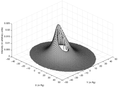
Figure 7: Unamplified (left) and amplified (right) brightness profile of the X-ray emitting region, corresponding to the highest peak in Fig. 5 (top right). The profiles are obtained using the ray tracing method (see, e.g., Popović et al. 2003a,b and references therein).

HMEs are asymmetric peaks in the light curves which depend not only on microlens parameters but also on the sizes of emitting regions in the following sense: the larger emitting regions are expected to produce smoother light curves and more symmetric peaks (Witt et al., 1995). Consequently, it can be expected that the majority of HMEs should be detected in X-ray light curves, less of them in UV and the smallest number in optical light curves. Therefore, we isolated only clearly asymmetric peaks in all light curves and measured their rise times $t_{HME}$ as the intervals between the beginning and the maximum of the corresponding microlensing events. In the case of Q2237+0305A we found the following number of HMEs: i) horizontal path: 13 in X-ray, 8 in UV and 7 in optical band, ii) diagonal path: 10 in X-ray, 7 in UV and 5 in optical band and iii) vertical path: 22 in X-ray, 12 in UV and 6 in optical band. In case of ”typical” lens these numbers are: i) horizontal path: 21 in X-ray, 10 in UV and 8 in optical band, ii) diagonal path: 30 in X-ray, 9 in UV and 7 in optical band and iii) vertical path: 18 in X-ray, 7 in UV and 4 in optical band.

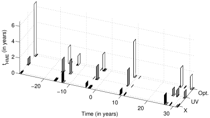
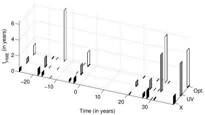
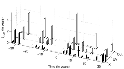
Figure 8: Rise times ($t_{HME}$) of high magnification events for all three spectral bands in the light curves of Q2237+0305A (Fig. 5). Top left panel corresponds to the horizontal, top right to the diagonal and bottom to the vertical path of accretion disc.

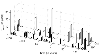
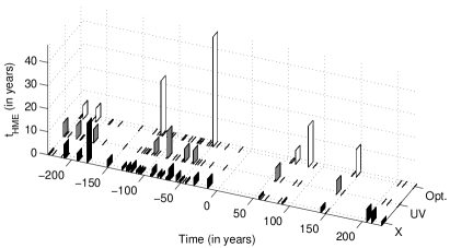
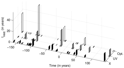
Figure 9: The same as in Fig 8. but for the light curves of ”typical” lens system (Fig. 6)

The average number of caustic crossings per unit length ($<N_{\rm caustic}>_{0}$) and per year ($<N_{\rm caustic}>_{y}$) are given in Table 2. This table also contains the average rise times ($<t_{HME}>$) in all three spectral bands, derived from the rise times ($t_{HME}$) of individual HMEs which are presented in Figs. 8 and 9 in the form of histograms. These results, as expected, show that the rise times are the shortest and the frequency of caustic crossings is the highest in the X-ray spectral band in comparison to the other two spectral bands. One can also see from Tables 1 and 2 that in the case of Q2237+0305A, the average rise times of HMEs for all three spectral bands (obtained from microlens magnification pattern simulations) are longer than both, caustic rise times (obtained from caustic simulations) and caustic times (calculated from equation (14)).

Microlensing can result in flux anomalies in the sense that different image flux ratios are observed in different spectral bands (Popović & Chartas, 2005; Popović et al., 2006b). As shown in Figs 2–6. the amplification in the X-ray band is larger and lasts shorter than it does in the UV and optical bands. Consequently, monitoring of lensed QSOs in the X-ray and UV/optical bands can clarify whether the flux anomaly is produced by CDM clouds, massive black holes or globular clusters (millilensing) or stars in foreground galaxy (microlensing).

5 Conclusion

In this paper we calculated microlensing time scales of different emitting regions. Using a model of an accretion disc (in the center of lensed QSOs) that emits in the X-ray and UV/optical spectral bands, we calculated the variations in the continuum flux caused by a straight-fold caustic crossing an accretion disc. We also simulated crossings of accretion discs over microlensing magnification patterns for the case of image A of Q2237+0305 and for a ”typical” lens system. From these simulations we concluded the following:

(i) one can expect that the X-ray radiation is more amplified than UV/optical radiation due to microlensing which can induce the so called ’flux anomaly’ of lensed QSOs.

(ii) the typical microlensing time scales for the X-ray band are on order of several months, while for the UV/optical they are on order of several years (although the time scales obtained from microlensing magnification pattern simulations are longer in comparison to those obtained from caustic simulations).

(iii) monitoring of the X-ray emission of lensed QSOs can reveal the nature of ’flux anomaly’ observed in some lensed QSOs.

All results obtained in this work indicate that monitoring the X-ray emission of lensed QSOs is useful not only to discuss the nature of the ’flux anomaly’, but also can be used for constraining the size of the emitting region.

References

- Bogdanov and Cherepashchuk (1995a) Bogdanov, M.B. and Cherepashchuk, A.M. 1995a, Astron. Lett., 21, 505
- Bogdanov and Cherepashchuk (1995b) Bogdanov, M.B. and Cherepashchuk, A.M. 1995b, Astron. Rep., 39, 779
- Chang & Refsdal (1984) Chang, K., Refsdal, S. 1984, A&A, 132, 168
- Chartas et al. (2002) Chartas, G., Agol, E., Eracleous, M., Garmire, G., Bautz, M. W., Morgan, N. D. 2002, ApJ, 568, 509
- Chartas et al. (2004) Chartas, G., Eracleous, M., Agol, E., Gallagher, S. C. 2004, ApJ, 606, 78
- Dai et al. (2003) Dai, X., Chartas, G., Agol, E., Bautz, M. W. & Garmire, G.P. 2003, ApJ, 589, 100
- Dai et al. (2004) Dai, X., Chartas, G., Eracleous, M., Garmire, G. P. 2004, ApJ, 605, 45
- Dobler & Keeton (2006) Dobler, G. and Keeton, C.R. 2006, MNRAS, 365, 1243
- Fabian et al. (1989) Fabian, A. C., Rees, M. J., Stella, L. & White, N. E. 1989, MNRAS, 238, 729
- Griest & Hu (1992) Griest, K. & Hu, W. 1992, ApJ, 397, 362
- Griest & Hu (1993) Griest, K. & Hu, W. 1993, ApJ, 407, 440
- Inoue & Chiba (2003) Inoue K.T. & Chiba M. 2003, ApJ, 591, L83
- Jovanović (2006) Jovanović, P. 2006, PASP, 118, 656
- Jaroszynski (1992) Jaroszyński, M., Wambsganss, J.W., Paczyński, B. 1992, ApJ, 396, L65.
- Kayser et al. (1986) Kayser, R., Refsdal, S. & Stabell, R. 1986, A&A, 166, 36
- Malzac (2007) Malzac, J. 2007, Mem. S.A.It. 78, 382
- Nandra et al. (1997) Nandra, K., George, I.M., Mushotzky, R.F., Turner, T.J. & Yaqoob, T. 1997, ApJ, 477, 602.
- Nandra et al. (1999) Nandra, K., George, I. M., Mushotzky, R. F., Turner, T. J., Yaqoob, T. 1999, ApJ 523, 17
- Oshima et al. (2001) Oshima, T., Mitsuda, K., Fujimoto R., Iyomoto N., Futamoto K., et al. 2001, ApJ, 563, L103
- Petters, Levine & Wambsganss (2001) Petters, A.O. Levine, H. & Wambsganss, J. 2001, Singular Theory and Gravitational Lensing, (Boston, Birkhäuser)
- Popović & Chartas (2005) Popović, L. Č., Chartas, G. 2005, MNRAS, 357, 135
- Popović et al. (2006a) Popović, L.Č., Jovanović, P., Mediavilla, E.G., Zakharov, A.F., Abajas, C., Muñoz, J.A. & Chartas, G. 2006a, ApJ, 637, 620
- Popović et al. (2006b) Popović, L.Č., Jovanović, P., Petrović, T., Shalyapin, V. N. 2006b, AN, 10, 981
- Popović et al. (2003a) Popović, L.Č., Mediavilla, E.G., Jovanović, P. & Muñoz, J.A. 2003, A&A, 398, 975
- Popović et al. (2003b) Popović, L.Č., Jovanović, P., Mediavilla, E.G. & Muñoz, J.A. 2003b, Astron. Astrophys. Transactions, 22, 719
- Popović et al. (2001) Popović, L., Č., Mediavilla, E.G., Muñoz J., Dimitrijević, M.S. & Jovanović, P. 2001, SerAJ, 164, 73
- Shakura & Sunayev (1973) Shakura, N.I. & Sunayev, R.A. 1973, A&A, 24, 337
- Schneider, Ehlers & Falco (1992) Schneider, P., Ehlers, J., Falco, E.E. 1992, Gravitational Lenses, (Springer, Berlin)
- Schneider & Weiss (1986) Schneider, P. & Weiss, A. 1986, A&A, 164, 237
- Schneider & Weiss (1987) Schneider, P. & Weiss, A. 1987, A&A, 171, 49
- Schneider & Weiss (1992) Schneider, P. & Weiss, A. 1992, A&A, 260, 1
- Totani (2003) Totani, T. 2003, ApJ, 586, 735
- Tadros, Warren & Hewett (1998) Tadros, H., Warren S. & Hewett, P. 1998, New Rev., 42, 115
- Tanaka et al. (1995) Tanaka, Y., Nandra, K., Fabian, A. C., Inoue, H., Otani, C., Dotani, T., Hayashida, K., Iwasawa, K., Kii, T., Kunieda, H., Makino, F., Matsuoka, M. 1995, Nat, 375, 659
- Treyer & Wambsganss (2004) Treyer, M. & Wambsganss, J. 2004, A&A, 416, 19
- Wambsganss et al. (1990a) Wambsganss, J., Paczyński, B. & Katz, N. 1990a, ApJ, 352, 407
- Wambsganss et al. (1990b) Wambsganss, J., Schneider, P. & Paczyński, B. 1990b, ApJ, 358, L33
- Witt et al. (1993) Witt, H.J., Kayser, R., Refsdal, S. 1993, A&A 268, 501
- Witt et al. (1995) Witt, H.J., Mao, S., Schechter, P. 1995, ApJ, 443, 18
- Wyithe & Turner (2002a) Wyithe, J.S.B. & Turner, E.L. 2002a, ApJ, 567, 18
- Wyithe & Turner (2002b) Wyithe, J.S.B. & Turner, E.L. 2002b, ApJ, 575, 650
- Zakharov (1994) Zakharov, A.F. 1994, MNRAS, 269, 283
- Zakharov (1995) Zakharov, A.F. 1995, A&A, 293, 1
- Zakharov (1997) Zakharov, A.F. 1997, Gravitational lenses and microlensing, (Janus-K, Moscow)
- Zakharov (2004) Zakharov, A.F. 2004, in Proc. of the 22nd Summer School and International Symposium on ”The Physics of Ionized Gases” ed. by L. Hadzievski, T. Gvozdanov, N. Bibic, AIP Conference Proceedings, 740, p. 398; astro-ph/0411611
- Zakharov (2007) Zakharov, A.F. 2007, Physics of Atomic Nuclei and Part., 70, 159
- Zakharov et al. (2003) Zakharov, A.F., Kardashev, N.S., Lukash, V.N. & Repin, S.V. 2003, MNRAS, 342, 1325
- Zakharov, Popović & Jovanović (2004) Zakharov, A.F., Popović L. Č. & Jovanović, P. 2004, A&A, 420, 881
- Zakharov, Popović & Jovanović (2005) Zakharov, A.F., Popović L. Č. & Jovanović, P. 2005, in Proc. of the IAU Symposium, eds. Y. Mellier and G. Meylan, 225, (Cambridge, UK, Cambridge University Press) p. 363
- Zakharov & Repin (1999) Zakharov, A.F. & Repin, S.V. 1999, Astronomy Reports, 43, 705
- Zakharov & Repin (2002) Zakharov, A.F. & Repin, S.V. 2002, Astronomy Reports, 46, 360
- Zakharov & Repin (2003a) Zakharov, A.F. & Repin, S.V. 2003a, A & A, 406, 7
- Zakharov & Repin (2003b) Zakharov, A.F. & Repin, S.V. 2003b, Astronomy Reports, 47, 733
- Zakharov & Repin (2003c) Zakharov, A.F. & Repin, S.V. 2003c, Nuovo Cimento, 118B, 1193
- Zakharov & Repin (2004) Zakharov, A.F. & Repin, S.V. 2004, Advances in Space Res., 34, 2544
- Zakharov & Repin (2005) Zakharov, A.F., Repin, S.V. 2005, Mem. S. A. It. della Supplementi, 7, 60
- Zakharov & Repin (2006) Zakharov A.F & Repin, S.V. 2006, New Astronomy, 11, 405
- Zakharov & Sazhin (1998) Zakharov, A.F. & Sazhin, M.V. 1998, Physics-Uspekhi, 41, 941