Ground-state reference systems for expanding correlated fermions in one dimension

Abstract

We study the sudden expansion of strongly correlated fermions in a one-dimensional lattice, utilizing the time-dependent density-matrix renormalization group method. Our focus is on the behavior of experimental observables such as the density, the momentum distribution function, and the density and spin structure factors. As our main result, we show that correlations in the transient regime can be accurately described by equilibrium reference systems. In addition, we find that the expansion from a Mott insulator produces distinctive peaks in the momentum distribution function at $k\approx\pm\pi/2$, accompanied by the onset of power-law correlations.

I Introduction

The nonequilibrium properties of strongly correlated electron systems are a challenging subject in need of a better understanding. While experimental studies in this area face difficulties in the solid state context, ultracold quantum gases provide a controlled way to address this difficult issue. For this reason, recent experiments employing out-of-equilibrium cold atom gases in optical lattices, which allows the realization of model Hamiltonians for strongly correlated particles (for a review, see, e.g., Ref. reviews ), have attracted considerable attention kinoshita06 ; greiner02 ; transport .

Among the fundamental questions recently addressed in these experiments is the issue of thermalization in isolated quantum systems kinoshita06 ; rigol07 ; cazalilla06 ; calabrese06 ; calabrese07 ; kollath07 ; eisler ; manmana07 ; cramer08 ; eckstein08 ; barthel08 . In the transient regime, quantum quenches have been shown to induce a collapse and revival of coherence properties greiner02 , and transport measurements in different lattice systems have unveiled the intriguing consequences of strong correlations transport . The important effects of interactions have been observed in the expansion of bosons in one-dimensional (1D) lattices as well emergence ; fermionization ; impurity ; disorder ; gangardt08 . In the expansion from a Mott insulator (MI) state, quasi-condensates at finite momenta emerge emergence , while in the hard-core regime, the expansion from a superfluid state leads to the dynamical fermionization of the bosonic momentum distribution function (MDF) fermionization . The latter is a generic feature of the expansion of harmonically trapped hard-core bosons in the absence of a lattice minguzzi05 . In addition, it has been shown in Ref. buljan08 that, independently of the initial interaction strength, a freely expanding Lieb-Liniger gas always enters a strongly correlated (hard-core like) regime. The expansion dynamics of strongly correlated fermions, which due to the spin-degree of freedom is expected to be richer, has not yet been addressed, and it is the objective of this work.

Concretely, we study the expansion of two-component interacting fermions in a 1D lattice. The ground state physics of these systems is characterized by a Tomonaga-Luttinger (TL) state with power-law decaying correlations at any incommensurate filling. At half-filling, a charge gap opens and the system exhibits quasi long-range antiferromagnetic correlations giamarchi . Here, we wish to elucidate how the initial state of the system, being either MI or TL, affects the expansion process. Identifying distinctive features for the MI is of much interest to experimentalists in the search for the fermionic MI state. However, our main objective is to shed light on the relation, if any, between these out-of-equilibrium systems and their equilibrium counterparts. As the main result of this work, we provide evidence that correlations measured in nonequilibrium are quantitatively described by appropriately chosen equilibrium reference systems.

The outline of the paper is the following. First, we describe the model and the numerical procedure in Sec. II. Section III contains our results on the time-evolution of density profiles and the momentum distribution function for both TL and MI initial states. In Sec. IV, we investigate what the possible relation to equilibrium system is, and we present a comparative analysis of spin and charge correlation functions. We also comment on the validity of our findings in other models, such as the Hubbard chain with a nearest-neighbor repulsion, which renders the model nonintegrable. We conclude with a summary of our results contained in Sec. V.

II Model and numerical method

The nonequilibrium dynamics is analyzed using the adaptive time-dependent density-matrix renormalization group method (tDMRG) white04 . We consider the 1D Hubbard model with nearest-neighbor hopping $t$ and an on-site Coulomb repulsion $U$:

$$H_{0}=-t\sum_{l=1}^{N-1}(c_{l+1,\sigma}^{\dagger}c_{l,\sigma}+\mathrm{h.c.})+U\sum_{l=1}^{N}n_{l,\uparrow}n_{l,\downarrow}\,.$$ (1)

$c_{l,\sigma}^{\dagger}$($c_{l,\sigma}$) is a fermion creation(annihilation) operator acting on site $l$, with (pseudo-)spin index $\sigma=\uparrow,\downarrow$, $n_{l,\sigma}=c_{l,\sigma}^{\dagger}c_{l,\sigma}$ is the corresponding density operator, and we define $n_{l}=\sum_{\sigma}n_{l,\sigma}$. $N$ denotes the number of sites, $a$ is the lattice constant, and open boundary conditions are imposed. We prepare an initial state with a filling $n_{\mathrm{init}}$ that is non-vanishing in only a portion of the system by applying a confining box-potential $H_{\mathrm{conf}}=\sum_{l=1}^{N}\epsilon_{l}n_{l}$. Hence, we have $H=H_{0}+H_{\mathrm{conf}}$, with $\epsilon_{l}=10^{6}t$ for $l\not\in[l_{0},l_{1}]$ and $\epsilon_{l}=0$ otherwise. At time $\tau=0$, we turn off $H_{\mathrm{conf}}$. $\tau$ is given in units of $1/t$, we set $\hbar$ to unity.

In our tDMRG runs we use a third-order Trotter-Suzuki time-evolution scheme with a time step of $\Delta\tau=0.005$. The discarded weight during the time-evolution is kept below $10^{-8}$. To simulate the longest time scales possible on a given system size before the particles are reflected at the boundaries, we select an asymmetric set-up and, hence, particles can only expand into one direction. We have checked that the same overall picture is observed in symmetric set-ups (see also Ref. emergence ).

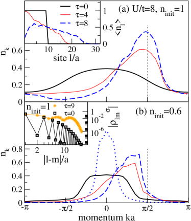
Figure 1: Expansion from a: (a) MI ($n_{\mathrm{init}}$=$1$; main panel: MDF; inset: density); (b) TL ($n_{\mathrm{init}}$=$0.6$); both at $U=8t$ and plotted at times $\tau=0,4,8$. Note that at $\tau\gtrsim 8$ and before the right boundary is reached, the MDF exhibits only small changes. Dotted line in (b): MDF of a reference system (see text in Sec. IV A for details) with $\langle n_{l}\rangle_{\mathrm{ref},\tau}=\langle n_{l}(\tau=8)\rangle$. Inset in (b): Decay of one-particle correlations during the expansion of the MI. The $\tau$=$0$ curve is for a $N$=$50$ system at half-filling. Dotted vertical lines in (a) and (b) denote $k=\pi/2$.

III The momentum distribution function

We first discuss the properties of the MDF $n_{k}$, computed from $n_{k}=(1/N)\sum_{l,m,\sigma}\exp[-ik(l-m)]\rho^{\sigma}_{lm}$, where $\rho^{\sigma}_{lm}=\langle c^{\dagger}_{l,\sigma}c_{m,\sigma}\rangle$ is the one-particle density matrix. In Fig. 1(a), we show the evolution of $n_{k}$ (main panel) and the density $\langle n_{l}\rangle$ (inset) for an initial MI state. The main panel reveals a peculiar behavior of $n_{k}$: as the Mott insulator melts, a peak develops at a finite momentum $k_{p}$. We further find that, for $U$ larger than the band-width $W=4t$, $k_{p}$ closely approaches $\pi/2$. This behavior resembles that of hard- and soft-core bosons emergence . Qualitatively, we understand this in terms of an energy argument: in the MI state with $U\gg W$, the total kinetic energy is close to zero. Hence, particles emitted into an empty lattice have a small average kinetic energy corresponding to a momentum $\pi/2$. As the Fermi statistics prohibits quasi-condensation into a single momentum state, $n_{k}$ becomes a broad function around $k_{p}\approx\pi/2$.

While the initial MI state is characterized by an exponential decay of one-particle correlations, i.e., $|\rho_{lm}^{\sigma}|$$\sim$$\exp(-|l-m|/\xi)$, $\xi$=const, we find that during the expansion, the system develops power-law correlations. In the inset of Fig. 1(b), we compare the $|\rho_{lm}^{\sigma}|$ of a MI in equilibrium with the correlations that emerge during its expansion, measured within the moving cloud. The inset reveals the weak decay of correlations during the expansion, consistent with a power law. One may associate the dynamical emergence of this power law with a metallization of the moving cloud, which, after the melting of the MI, starts behaving as an inhomogeneous metal. As of now, our numerical analysis is restricted to a small number of particles and time scales of $\tau\sim 15$ only, which prevents us from extracting, e.g., exponents of the power laws. Note, though, that in the case of free fermions expanding from an insulating state with $n_{\mathrm{init}}=1$, i.e., a state with no off-diagonal correlations, the emergence of power laws has been established for a large number of particles and hence over substantially larger distances than in the present work rigol05 .

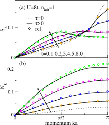
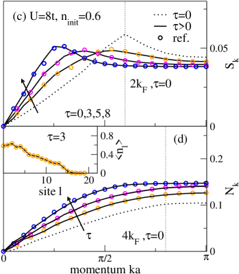
Figure 2: (Color online) Time evolution of (a) the kinetic energy $T_{\mathrm{kin}}$ and (b) the potential energy $E_{\mathrm{init}}$ for the expansion from an initial TL state with $U=8t$, $n_{\mathrm{init}}=0.6$ (dashed lines) and the corresponding reference systems (squares). Panel (a) further shows the kinetic energy of the cloud and of the reference systems as estimated from Eq. (5) (thick dotted line and stars, respectively) as well as our approximate results for the kinetic energy $T_{\mathrm{kin}}^{\mathrm{Gal}}$ associated with the center-of-mass motion of the cloud [solid line in (a)]. See the text in Sec. IV C for definitions and details.

In the main panel of Fig. 1(b), we show the evolution of the MDF starting from a TL state with $n_{\mathrm{init}}<1$. In this case, the initial state has a well-defined Fermi momentum and a power-law decay of correlations giamarchi . Such decay is preserved during the expansion. Moreover, $n_{k}$ also exhibits a peak, but at a momentum $k_{p}<\pi/2$ ($k_{p}$ increases as $n_{\mathrm{init}}\to 1$). Another property of this peak, distinguishing it from the peak formed after the melting of the MI, is that it exhibits a much sharper edge at the large momentum side, reminiscent of a Fermi edge.

From the previous analysis, we conclude that if $n_{k}$ could be experimentally studied during the expansion in the strongly correlated regime, then the emergence of peaks at $k=\pm\pi/2$ in the fermionic MDF would serve to identify the presence of a Mott insulator in the initial state. The experimental challenge is to independently control the trapping potential and the lattice kinoshita04 ; clement05 ; fort05 . This has been achieved in the experimental study of disordered ultracold Bose gases in both 1D optical lattices clement05 and homogeneous 1D systems fort05 .

At this point we would like to emphasize that the physics of our expanding system is different from the one found in theoretical studies of strongly correlated systems in 1D lattices undergoing a relaxation following a quantum quench rigol07 ; kollath07 ; manmana07 . In the latter, correlations have been found to decay faster than with a power law (sometimes clearly exponentially) calabrese06 ; rigol07 ; kollath07 ; manmana07 , while in our moving clouds we find power-law decaying correlations [inset of Fig. 1(b)]. In addition, after the relaxation to a steady state, one can ask the question of what statistical ensemble may best describe physical observables, but here we are solely concerned with the transient regime, i.e., a regime in which statistical ensembles do not provide us with insights into the behavior of physical observables.

IV Ground-state reference systems

IV.1 Construction of reference systems

Our results thus far have singled out a noticeable property of these systems during their expansion: independently of the initial ground state, power laws are observed in the nonequilibrium dynamics. In 1D systems in equilibrium, power-law correlations are only seen in the ground state, as finite temperatures introduce a cut-off at large distances, followed by an exponential decay giamarchi . Hence, one may wonder whether a system out of equilibrium can in some way resemble the ground state of a system in equilibrium. A natural choice for such a reference state is the ground state of a system that has exactly the same density distribution as the time evolving state, i.e.,

$$\langle n_{l}\rangle_{\textrm{ref},\tau}=\langle n_{l}(\tau)\rangle\,,$$ (2)

for all sites $l$. Hence, a reference system has to be determined at each given time. We construct such reference states by self-consistently computing a set of onsite energies $\epsilon_{l}$ in

$$H_{\mathrm{ref}}=H_{0}+\sum_{l=1}^{N}\epsilon_{l}n_{l}$$ (3)

with $H_{0}$ from Eq. (1) such that at a desired time, the density profile $\langle n_{l}(\tau)\rangle$ is reproduced, while keeping $t$ and $U$ fixed. Once the density has converged within an error of

$$\delta n_{\tau}=\sum_{l}|\langle n_{l}(\tau)\rangle-\langle n_{l}\rangle_{\textrm{ref},\tau}|/\sum_{l}\langle n_{l}(\tau)\rangle<10^{-3}\,,$$ (4)

we compare quantities of interest in both systems.

IV.2 Spin and charge structure factor

We now turn to the comparative analysis of correlation functions. We compute the spin-spin ($S_{k}$) and density-density ($N_{k}$) structure factors, which are the Fourier transforms of the spin-spin ($S_{lm}=\langle S_{l}^{z}S_{m}^{z}\rangle$) and density-density ($N_{lm}=\langle{n}_{l}{n}_{m}\rangle-\langle{n}_{l}\rangle\langle{n}_{m}\rangle$) correlations, respectively. The spin operator is defined as $S_{l}^{z}=(n_{l,\uparrow}-n_{l,\downarrow})/2$. In equilibrium and for a homogeneous system, $S_{k}$ peaks at $2k_{F}$ while $N_{k}$ exhibits a kink at $4k_{F}$ giamarchi , where $k_{F}=\pi n/2$ is the Fermi momentum. Consistently, for the two cases $n_{\mathrm{init}}=1$ and $n_{\mathrm{init}}=0.6$ shown in Figs. 2(a) and 2(c), respectively, $S_{k}(\tau=0)$ [dotted lines] peaks at $k=\pi$ and $k=\pi\,0.6$, while $N_{k}$ in the case of $n_{\mathrm{init}}=0.6$ has a weak kink at $k=2\pi\,0.6$ [dotted line in Fig. 2(d)]. During the expansion, the peak in $S_{k}$ shifts to smaller momenta and the maximum is less sharp, as shown in Figs. 2(a) and 2(c) [solid lines]. Qualitatively, we understand this behavior in terms of the decrease of the average density during the expansion into the initially empty lattice, giving rise to a shift of the $2k_{F}$ peak in $S_{k}$ and a broadening due to the inhomogeneity. Further, we propose an operational definition of a Fermi-momentum $k_{F}^{\tau}$ in the expanding clouds by taking the position of the peak in $S_{k}$, yielding $2k_{F}^{\tau}$. This supports the use of the term “metallization” for the process that fermions escaping from a MI undergo.

The density correlation $N_{k}$ does not show any particular features during the time-evolution, as the kink is washed out due to the inhomogeneity. $N_{k}$ increases monotonously with time, reflecting an increase of the overall charge fluctuations, due to the closing of the charge gap as the MI melts.

Our most remarkable finding, and thus the key result of this work, is the excellent agreement seen in Fig. 2 for $S_{k}$ and $N_{k}$ between the expanding cloud – a genuine nonequilibrium situation – and the inhomogeneous reference systems, which are in their ground state (circles in Fig. 2). We are therefore led to conclude that, during the expansion, spin and charge correlations out of equilibrium are, to a very good approximation, the same functionals of the density as the ones in equilibrium systems in the ground state.

IV.3 Time-evolution of kinetic and potential energy

Intuitively, we expect that our way of preparing the reference systems must yield properties similar to those of the moving clouds on short time scales. However, the agreement between the clouds and the equilibrium systems exists both at short and long times, and is thus preserved during the expansion into the empty lattice. A noticeable difference exists between $n_{k}$ of the moving clouds and $n_{k}$ of the corresponding reference systems. As discussed before, $n_{k}$ of the expanding cloud has a finite-momentum maximum, which is also present in the symmetric expansion, while $n_{k}$ of the reference system in its ground state is symmetric around $k=0$ [see dotted line in Fig. 1(b)]. Hence, observables related to $n_{k}$ cannot be accounted for with this procedure.

Our previous findings on the spin and density structure factors may seem puzzling: at any given time, the sum of the kinetic, $T_{\mathrm{kin}}$, and interaction energy $E_{\mathrm{int}}$ of the time-evolving state is much higher than the energy of the reference system, which, having the same density profile, is in its ground state. This difference grows with time. In the case of $n_{\mathrm{init}}=0.6$ and $U=8t$, we have $E_{0}=T_{\mathrm{kin}}+E_{\mathrm{int}}=-6.86t$, which of course is a constant in time. At $\tau=8$, this splits into $T_{\mathrm{kin}}=-t\sum_{l,\sigma}\langle c_{l+1,\sigma}^{\dagger}c_{l,\sigma}+h.c.\rangle=-6.97t$ and $E_{\mathrm{int}}=U\sum_{l}\langle n_{l,\uparrow}n_{l,\downarrow}\rangle=0.11t$. In contrast, for the reference system, we find $T_{\mathrm{kin}}^{\mathrm{ref}}=-10.93t$, and $E_{\mathrm{int}}^{\mathrm{ref}}=0.18t$, adding up to $E_{0}^{\mathrm{ref}}=-10.75t$. Thus, the main difference is due to the kinetic energies.

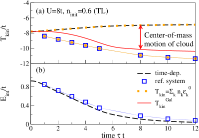
Figure 3: (Color online) Time evolution of (a) the kinetic energy $T_{\mathrm{kin}}$ and (b) the potential energy $E_{\mathrm{init}}$ for the expansion from an initial TL state with $U=8t$, $n_{\mathrm{init}}=0.6$ (dashed lines) and the corresponding reference systems (squares). The plot further shows the kinetic energy of the cloud as estimated from Eq. (5) [thick dotted line and stars] as well as our approximate results for the kinetic energy $T_{\mathrm{kin}}^{\mathrm{Gal}}$ associated with the center-of-mass motion of the cloud (solid line). See text in Sec. IV.3 for definitions and details.

We argue that both systems can be related by a Galilean transformation and, thus, understand why their structure factors are similar. This means that the difference between the kinetic energies $T_{\mathrm{kin}}$ and $T_{\mathrm{kin}}^{\mathrm{ref}}$ is mainly due to the average momentum of the moving cloud [$k_{0}=\sum_{k}kn_{k}/\sum_{k}n_{k}$], i.e., that $T_{\mathrm{kin}}^{\mathrm{ref}}\approx T_{\mathrm{kin}}^{\mathrm{Gal}}$, the latter being the kinetic energy of the particles in a reference frame moving with the cloud. To prove this, we first notice that, using the MDF, the kinetic energy can be estimated as

$$T_{\mathrm{kin}}=\sum_{k}n_{k}\epsilon_{k}^{0}\,,$$ (5)

where $\epsilon_{k}^{0}=-2t\cos k$ is the dispersion relation in the noninteracting case. This assumption leads to $T_{\mathrm{kin}}\approx-6.97t$ and $T_{\mathrm{kin}}^{\mathrm{ref}}\approx-10.93t$, as estimates for the kinetic energy of the expanding and reference systems at $\tau=8$ ($n_{\mathrm{init}}=0.6$, $U=8t$), respectively. Both values are very close to the exact results presented before. We then compute $T_{\mathrm{kin}}^{\mathrm{Gal}}=\sum_{k}n_{k}\epsilon_{k-k_{0}}^{0}=-10.15t\approx T_{\mathrm{kin}}^{\mathrm{ref}}$ at $\tau=8$, which corroborates our interpretation: the energy difference is mostly due to the finite momentum of the cloud, and not due to contributions of the internal kinetic or interaction energy. This picture is further supported by Fig. 3 that contains the time-evolution for $T_{\mathrm{kin}}$, $E_{\mathrm{int}}$, $T_{\mathrm{kin}}^{\mathrm{ref}}$, and $T_{\mathrm{kin}}^{\mathrm{Gal}}$ for the parameters discussed in this section.

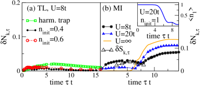
Figure 4: (Color online) Relative deviation of the density structure factor vs. time [see Eq. (6)], for: (a) $n_{\mathrm{init}}$=$0.4,0.6$ and a harmonic trap (8 fermions, $V_{\mathrm{trap}}$=$0.02t$, $U$=$8t$) and (b) $n_{\mathrm{init}}$=$1$ ($U/t$=$8,20,\infty$). We estimate our calculation of $\delta N_{k,\tau}$ to have an accuracy of $\pm 0.01$ in the worst case. Inset in (b): density in the leftmost site vs. time for $U=20t$.

IV.4 Breakdown of the ground-state reference system description

It is next important to identify conditions for a breakdown of the reference-system description. To this end, we study the relative difference between the time-dependent and the reference systems’ density structure factors,

$$\delta N_{k,\tau}={\sum_{k}|N_{k}(\tau)-N_{k,\tau}^{\mathrm{ref}}|}/{\sum_{k}N_{k}(\tau)}.$$ (6)

The corresponding errors in $S_{k}$ are smaller than those in $N_{k}$, and we thus concentrate on the latter. Let us start with the initial TL. We consider two cases: first, $n_{\mathrm{init}}<1$ in a box trap [see Fig. 2(d)]. Second, as such a set-up is more realistic to account for experiments, we follow the evolution of fermions escaping from a harmonic trap $V_{\mathrm{trap}}\sum_{l}(l)^{2}n_{l}$. From the results displayed in Fig. 4(a), our key observation is that $\delta N_{k,\tau}\lesssim 0.02$ remains very small in both cases. Hence, for an initial TL state and for both $N_{k}$ and $S_{k}$, the description given by the equilibrium systems is very good up to the largest times simulated.

We next turn to the case of an initial MI region, and present results in Fig. 4(b) for $U=8t,20t,\infty$. The $U=\infty$ case is treated with exact diagonalization, after mapping the charge sector of our two-component fermion system to spinless fermions giamarchi . A behavior similar to the TL case is found at times $\tau\lesssim 5$, with $\delta N_{k,\tau}\lesssim 0.04$. However, for times after the melting of the MI region [$\tau\gtrsim 5$, see the inset in Fig. 4(b)], a substantial increase of $\delta N_{k,\tau}$ becomes evident, as shown in Fig. 4(b). Thus, for the MI expansion, reference systems work well only up to the point at which the Mott insulator totally melts.

This deviation of the time-dependent data from the reference systems is associated to the appearance of particular coherence properties in the portion left behind by the moving cloud after the melting of the MI, a feature that is not captured by the reference systems. To substantiate this interpretation, we present results for the decay of $N_{ij}$ in the $U=\infty$ limit in Fig. 5. In that limit, we are able to exactly treat arbitrary time scales for both large number of particles and a large system size. The data displayed in Fig. 5 are for 500 spinless fermions expanding from a MI region into a lattice of 2000 sites.

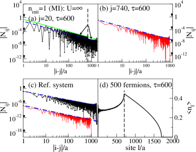
Figure 5: (Color online) $U=\infty$, 500 particles, $n_{\mathrm{init}}=1$. (a) Decay of $|N_{ij}|$ at time $\tau=600$ for $j=20$ (solid line with squares). The dashed lines are fits to the envelope of $|N_{ij}|$ using $f(|i-j|)=\alpha|i-j|^{-\beta}$. Note that two regions appear that are described by the same exponent $\beta$, but a different prefactor $\alpha$. (b) The same as in (a), but for $j=740$ (solid line). Note that we plot correlations for $i>j$ only. (c) Density-density correlations measured in the reference system for $\tau=600$, with $j=20$ (solid line with squares) and $j=740$ (solid lines). The latter curve has been offset for clarity. The dashed-dotted lines are the fits from panels (a) and (b). (d) Density profile at time $\tau=600$. Vertical, dashed lines in (a) and (d) mark $i=705$, separating the regions with different prefactors in the power-law decay of $|N_{ij}|$ at the time $\tau=600$ considered in this plot.

In Fig. 5, we measure the density-density correlations at a time $\tau=600$, at which the initial Fock state has already completely melted. Figure 5(d) shows the density profile at this time and from that plot, we see that at time $\tau=600,$ $i\approx 705$ separates the front of fast particles from slower ones, as indicated by the vertical dashed line in the figure. Panels (a) and (b) show $|N_{ij}|$ for $i>j$, and $j=20$ and $j=740$, respectively, i.e., measured from behind and from inside the moving front [Fig. 5(d)]. While in the latter case, clearly a unique power-law decay of $|N_{ij}|$ is observed, the former case is more involved. There, the envelope of the correlator also decays according to $|N_{ij}|=\alpha\,|i-j|^{\beta}$, yet for $i\lesssim 705$ and $i\gtrsim 705$, a different prefactor $\alpha$ is found. These are the two regions in Fig. 5(a) indicated by the arrows. The exponent $\beta=2K$ is universal and expected to be $\beta=2$ since the Luttinger parameter $K$ of spinless fermions is $K=1$, but the prefactor – in the ground-state – is essentially a function of the average density, or the Fermi momentum, respectively giamarchi . The density-density correlations therefore exhibit a distinctly different behavior comparing the moving front of fast particles ($i\gtrsim 705$) and those left behind ($i\lesssim 705$). It is exactly this step-like feature, i.e., the sudden change in the prefactor of the power law followed by $|N_{ij}|$, that is not captured by the reference systems. This is revealed in Fig. 5(c), which shows the $|N_{ij}^{\mathrm{ref}}|$ as measured in the reference system constructed for time $\tau=600$, for both $j=20$ and $j=740$. The plot includes the fits to $|N_{ij}|$ from panels (a) and (b) [dot-dashed lines]. While for $j=740$, $|N_{ij}|$ is well described by the reference systems, $|N_{ij}^{\mathrm{ref}}|$ with $j=20$ does not show the step like feature observed in the moving cloud, as the reference systems fail to account for the separation of particles moving at different velocities.

For this reasoning to apply, it is important to realize that such a separation of velocities as reflected in the two prefactors to the power-law decay is not observed in the expansion from a TL state. There, a power-law with a single pair of exponent and prefactor governs the decay of one-particle and density-density correlations fermionization .

IV.5 Nonintegrable systems

Beyond the case of the Hubbard model Eq. (1), the question arises whether non-stationary states of other model Hamiltonians may as well be described by ground-state reference systems. Conceptually, one may wonder whether integrability plays a role or not.

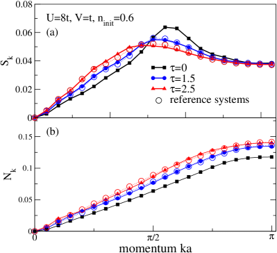
Figure 6: (Color online) Structure factor for (a) spin and (b) density correlations for the extended Hubbard model with $U=8t$, $V=t$. The results are for the expansion from an initial state with $n_{\mathrm{init}}=0.6$ and 6 particles. Time-dependent data are represented with solid lines and solid symbols, the corresponding ground state reference system ones are displayed with open circles.

While a full account of these interesting issues is beyond the scope of the present work, we wish to at least comment on one additional model, the extended Hubbard model. In addition to the terms given in Eq. (1), this model incorporates a nearest-neighbor repulsion $H_{\mathrm{2}}$:

$$H_{2}=V\sum_{l=1}^{N-1}n_{l}n_{l+1}\,.$$ (7)

The nearest-neighbor interaction both renders the system nonintegrable and induces additional phases at half-filling. For $V<U/2$, the system is a Mott insulator, while a large $V$ drives the system into a charge-density wave phase jeckelmann02 . Here we focus on the numerically less demanding case of the expansion from an initial state with an incommensurate filling of $n_{\mathrm{init}}=0.6$. We postpone the discussion of the MDF to a future publication, but rather compute the spin and charge structure factors for both the expanding system and the reference systems constructed according to the prescription of Sec. IV.1. The results for $U=8t$ and $V=t$ are collected in Fig. 6, and we note that in this case, we consider the expansion from a box trap only.

Our observation is that the reference systems still provide a very good approximation to the time-dependent correlations. Moreover, the agreement remains to be much better for the spin structure factor than for the charge structure factor. Future work will have to clarify whether the reference system description breaks down as $V$ is increased. In conclusion, we find that the reference system description does not seem to be crucially dependent on integrability, and we expect a similar picture to emerge in other models.

IV.6 Discussion: Relation to density functional theory

Our main results have shown that starting from a Mott-insulator, the temporal evolution of spin and density correlation functions are very accurately described by the ground-state of reference systems defined at each instant of time so that they have the same density distribution as the time evolving system. Such a description deteriorates after the Mott insulating region has totally melted. On the other hand, for systems starting with densities $n_{\mathrm{init}}<1$, the description with reference systems remains valid up to the largest times reached in our simulations. These results explicitely show that the correlation functions studied here are functionals of the density, a fact that is in accordance with density functional theory (DFT) for time-dependent systems dft ; tdft .

DFT considers, both for the ground state and time-dependent situations, this kind of Hamiltonian dft ; tdft :

$$H=H_{\mathrm{kin}}+H_{\mathrm{Coulomb}}+H_{\mathrm{ext}}\,\,,$$ (8)

i.e., one separates the Hamiltonian into kinetic energy, the interaction energy due to Coulomb interactions, and an external potential. We should here remark that in our case, the time-dependent external potential is discontinuous at time $\tau=0$, as we use $H_{\mathrm{ext}}=H_{\mathrm{conf}}$ at time $\tau=0$ and $H_{\mathrm{ext}}=0$ for $\tau>0$. Therefore, it does not strictly comply with the assumptions needed to prove the Runge-Gross theorem runge84 , i.e., the external potential needs to be analytical around $\tau=0$.

However, and most importantly, the reference systems explicitely provide the required functionals, namely the correlation functions in the respective ground-states. This is, to our opinion, a rather surprising and nontrivial fact that the correlations of a genuinely non-stationary state can be quantitatively described by equilibrium systems. Moreover, since they are in their ground-state, this suggests that a minimum principle is at work here. As shown in Sec. IV.5, these conclusions are not restricted to the pure Hubbard-model, i.e., they are not a consequence of integrability. Therefore, we expect that they hold in general.

V Summary

In this work, we have identified several remarkable and unexpected properties of fermions expanding into an empty lattice. These include the emergence of coherence as well as well as an accumulation of particles at momentum $\pi/2$ in the expansion of particles coming from a MI region. In particular, we have shown that correlation functions of expanding, interacting fermions can be accurately described by equilibrium reference systems in their ground state. These results are expected to qualitatively carry over to other models as well, and certainly also apply to the case of hard-core bosons.

- (1) I. Bloch, J. Dalibard, and W. Zwerger, arXiv:0704.3011.
- (2) T. Kinoshita, T. Wenger, and D. S. Weiss, Nature (London) 440, 900 (2006); S. Hofferberth, I. Lesanovsky, B. Fischer, T. Schumm, and J. Schmiedmayer, Nature (London) 449, 324 (2007).
- (3) M. Greiner, O. Mandel, T. W. Hänsch, and I. Bloch, Nature (London) 419, 51 (2002).
- (4) H. Moritz, T. Stöferle, M. Köhl, and T. Esslinger, Phys. Rev. Lett. 91, 250402 (2003); H. Ott, E. de Mirandes, F. Ferlaino, G. Roati, G. Modugno, and M. Inguscio, ibid. 92, 160601 (2004); C. D. Fertig, K. M. O’Hara, J. H. Huckans, S. L. Rolston, W. D. Phillips, and J. V. Porto, ibid. 94, 120403 (2005); J. Mun, P. Medley, G.K. Campbell, L. G. Marcassa, D.E. Pritchard, and W. Ketterle, ibid. 99, 150604 (2007); N. Strohmaier, Y. Takasu, K. Günter, R. Jördens, M. Köhl, H. Moritz, and T. Esslinger, ibid. 99, 220601 (2007).
- (5) M. Rigol, V. Dunjko, V. Yurovsky, and M. Olshanii, Phys. Rev. Lett. 98, 050405 (2007); M. Rigol, A. Muramatsu, and M. Olshanii, Phys. Rev. A 74, 053616 (2006).
- (6) M. A. Cazalilla, Phys. Rev. Lett. 97, 156403 (2006).
- (7) P. Calabrese and J. Cardy, Phys. Rev. Lett. 96, 136801 (2006).
- (8) P. Calabrese and J. Cardy, J. Stat. Mech.: Theory Exp., P06008 (2007).
- (9) C. Kollath, A. M. Läuchli, and E. Altman, Phys. Rev. Lett. 98, 180601 (2007).
- (10) S. R. Manmana, S. Wessel, R. M. Noack, and A. Muramatsu, Phys. Rev. Lett. 98, 210405 (2007).
- (11) V. Eisler and I. Peschel, J. Stat. Mech., P06005 (2007); V. Eisler, D. Karevski, T. Platini, and I. Peschel ,J. Stat. Mech., P01023 (2008).
- (12) M. Cramer, C. M. Dawson, J. Eisert, and T. J. Osborne, Phys. Rev. Lett. 100, 030602 (2008).
- (13) M. Eckstein and M. Kollar, Phys. Rev. Lett. 100, 120404 (2008).
- (14) T. Barthel and U. Schollwöck, Phys. Rev. Lett. 100, 100601 (2008).
- (15) M. Rigol and A. Muramatsu, Phys. Rev. Lett. 93, 230404 (2004); K. Rodriguez, S.R. Manmana, M. Rigol, R.M. Noack, A. Muramatsu, New J. Phys. 8, 169 (2006).
- (16) M. Rigol and A. Muramatsu, Phys. Rev. Lett. 94, 240403 (2005); Mod. Phys. Lett. B 19, 861 (2005).
- (17) A. Micheli, A. J. Daley, D. Jaksch, and P. Zoller, Phys. Rev. Lett. 93, 140408 (2004); A. Micheli and P. Zoller, Phys. Rev. A 73, 043613 (2006).
- (18) B. Horstmann, J. I. Cirac, and T. Roscilde, Phys. Rev. A 76, 043625 (2007).
- (19) D.M. Gangardt and M. Pustilnik, Phys. Rev. A 77, 041604(R) (2008).
- (20) A. Minguzzi and D. M. Gangardt, Phys. Rev. Lett. 94, 240404 (2005).
- (21) H. Buljan, R. Pezer, and T. Gasenzer, Phys. Rev. Lett. 100, 080406 (2008).
- (22) See, e.g.: T. Giamarchi, Quantum physics in one dimension, Clarendon Press, Oxford, 2004.
- (23) S. R. White and A. E. Feiguin, Phys. Rev. Lett. 93, 076401 (2004); A. Daley, C. Kollath, U. Schollwöck, and G. Vidal, J. Stat. Mech.: Theory Exp., P04005 (2004).
- (24) M. Rigol and A. Muramatsu, J. Low Temp. Phys. 138, 645 (2005).
- (25) T. Kinoshita, T. Wenger, and D. S. Weiss, Science 305, 1125 (2004).
- (26) D. Clément, A. F. Varón, M. Hugbart, J. A. Retter, P. Bouyer, L. Sanchez-Palencia, D. M. Gangardt, G. V. Shlyapnikov, and A. Aspect, Phys. Rev. Lett. 95, 170409 (2005).
- (27) C. Fort, L. Fallani, V. Guarrera, J. E. Lye, M. Modugno, D. S. Wiersma, and M. Inguscio, Phys. Rev. Lett. 95, 170410 (2005).
- (28) See, e.g., E. Jeckelmann, Phys. Rev. Lett. 89, 236401 (2002).
- (29) R. M. Dreizler and E.K. Gross, Density Functional Theory (Springer, Berlin, 1990).
- (30) E.K.U Gross and K. Burke, Lect. Notes. Phys. 706, 1 (2006).
- (31) E. Runge and E.K.U. Gross, Phys. Rev. Lett. 52, 997 (1984).