Gravitation model for spatial network based on the heterogeneous node

Abstract

In this paper we consider nodes in network are heterogeneous and the link between nodes is caused by the potential dynamical demand of the nodes. Such demand can be measured by gravitation which increases with the heterogeneous strength of node and decreases with the geographical distance. Based on this, we propose a new model for spatial network from the view of gravitation. The model is to maximize the potential dynamical demand of the whole network, indicating the possible maximal efficiency of the network and the highest profits that operators may gain. The model can vary its topology by changing two parameters. A simulation for the Chinese city airline network is completed. In the end of this article we discuss the significance and advantage of the heterogeneous nodes.

I Introduction

Since the initial studies on the small-world phenomenon were presented by Watts and Strogatz WS and the scale-free property by Barabasi and Albert BA , a lot of achievements on complex network have been gotten. And our research group have also studied some features on network hdd . Most previous works focus on the topological properties of the network. However many networks are those embedded in the real space whose nodes occupy a precise position in Euclidean space and whose links are constrained by the geographic distance. Some typical examples are communication networks RA ; VM ,electric power grids RIG , transportation systems ranging from river Pitts to airport Amaral ; Barrat ; Smith , street Crucitti , railway and subway Latora . In these spatial networks, geographical factor is demonstrated to play an important role on the network’s topology. Very recently a few models for the spatial network have been proposed. Some models consider both the topological and spatially preferential attachment Waxman ; Yook ; xie while others take some optimal mechanism Carlson ; Gastner1 ; Gastner2 . These works provide some guidelines in network design. On the other hand, the geographic effects on the efficiency or traffic of the network are paid less attention. However traffic on network is very important since it represents the efficiency of the network. Therefore, if the traffic between nodes can be predicted in some way, it is likely to construct the network efficiently. Inspired by this idea and its significance, we proposed a new spatial network model. The model is to maximize the whole expected traffic of the network, indicating the highest efficiency that the network may gain. The expected traffic is measured by the gravitation. Especially, we propose the heterogeneity of nodes and argue its significance on the network’s topology and dynamics.

II Heterogeneous nodes and gravitation

In the previous studies on complex networks, nodes are usually identical. However in the real network, situations are very different. In the city airline network, each node (city) has different population or economic level and such difference can be very obvious. As is shown in Fig. 1, the population of the Chinese city follows approximately a two-regime power-law distribution, indicating a large variance of the grade of the city. The population can be considered as the own attribute of node which is distinguished from others and indicates its own grade. Such phenomenon also exists in the Internet and World Wide Web-routers with different capacity and webs with heterogeneous resources. Thus a node usually has its own attribute, grade or energy indicating the heterogeneity. We define heterogeneous strength to describe this heterogeneity, denoted by M. In addition, we found the heterogeneous strength(i.e.the population of city node) have positive correlation with the degree of city node, as is shown in Fig. 2.

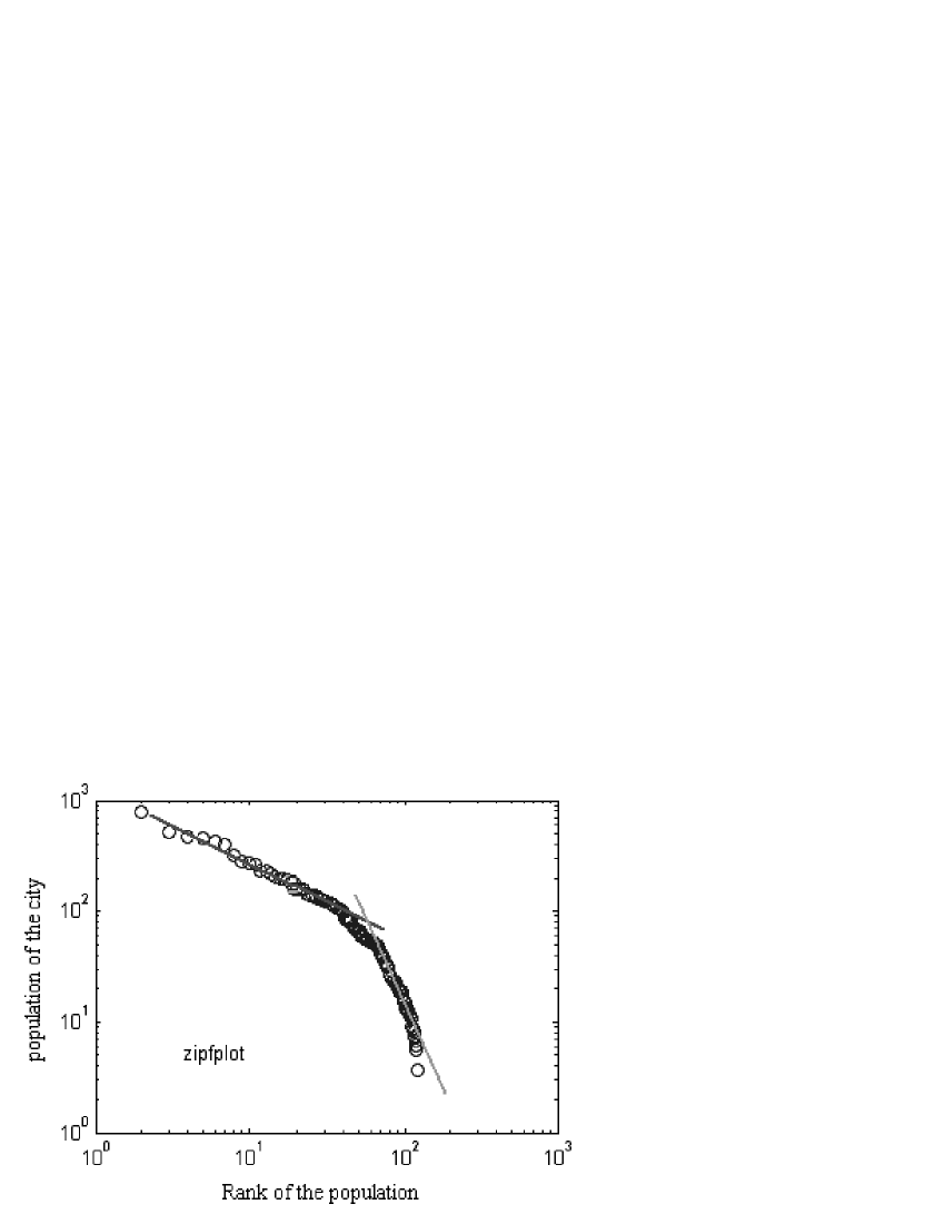
Figure 1: The Zipf-type plot distribution of the population of Chinese cities. It approximately follows a two-regime power-law distribution indicating the large variance of the heterogeneous strength. The population information is obtained from Ref. China City

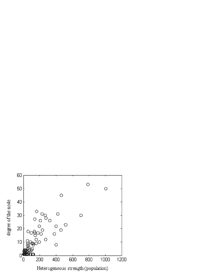
Figure 2: The correlation of the degree and the population of the city in Chinese city airline network. It shows the heterogeneous strength has a positive correlation with the node’s degree.The degree information is obtained from URL: http://www.caac.gov.cn.

Now we consider a network is composed of a group of nodes and links. Links connect every node and realize the dynamics among them. If two nodes with no dynamics between them, the link of the two vertices can be thought unwanted. In a circuit network, for example, a lead equals to disconnection if its current is 0. In other words, it is the dynamical demand between nodes that causes the link. Such demand is fulfilled when nodes are connected and can be measured by the weight. However, the demand still exists even though the vertices are not connected.

Consider a network with n nodes and 0 edges. Every two nodes have their demand for some information exchange. What we care is which of these demands are the most exigent. If such information is obtained in advance, the network will be constructed efficiently by preferentially investing those pairs of nodes with great demand. To measure such demand, some of its properties should be discussed first: (1) In a spatial network, links are constrained by the geographic factors and the travel cost among the nodes increases with the distance Gastner2 . So for the spatial network, the demand of nodes is assumed to decrease with the distance between them. (2)Since such demand can be measured by weight after nodes are connected, we hope it has some similar features with the real weight. In some kinds of network, such as the airline network, the weight has the form as follows, $<w_{ij}>\sim x_{ij}(k_{i}k_{j})^{\alpha}$ AMRA ; PJM , where $k_{i}$ and $k_{j}$ are the degree of node i and j. Since degree k has a positive correlation to heterogeneous strength M as we mentioned above, it is reasonable to suppose such demand is proportional to $(M_{i}M_{j})^{\alpha}$. The above two points indicate that the potential dynamical demand between two nodes can be described by the following equation,

$$G_{ij}=K\frac{{M_{i}^{\alpha}}{M_{j}^{\alpha}}}{D_{ij}^{\gamma}},$$ (1)

Equation (1) reminds us of the Newton’s gravitation equation. From the gravitation view, the dynamical demands is considered to make the nodes magnetize with each other and get the link when the gravitation $G_{ij}$ is great enough. However such demand is potential, it is a measurement of the expected traffic which is a prediction of the real traffic.

III Gravitation model for spatial network

We use the gravitation equation (1) to measure the potential dynamical demand. Rewrite equation (1),

$$G_{ij}=K\frac{{M_{i}^{\alpha}}{M_{j}^{\alpha}}}{D_{ij}^{\gamma}},$$ (2)

where K is a constant coefficient. $M_{i}$, $M_{j}$ are the heterogeneous strength of node i and node j. Exponents $\alpha$, $\gamma$ determine the impact of $D_{ij}$ and M on the gravitation. If $\gamma$ takes great value, the network is expected to be strongly constrained by the geographic distance. On the other hand, larger value of $\alpha$ means the dominant impact of the heterogeneous strength on the topology of the network. The topology of the simulated network is changed by varying parameters $\alpha$ and $\gamma$. The cost of constructing the network is defined as the total number of the network’s edges. It is reasonable for the airline networks whose cost and expense are related to the total hops. But for road network whose expense depends on the Euclidean distance, such definition seems unconvinced. However, later discussion will be revealed that such definition is still reasonable. Now suppose there are n nodes distributed on a two-dimension plane. The heterogeneous strength and coordinates of each node are known. By equation (2), the gravitation $G_{ij}$ of any two nodes can be calculated. We connected preferentially those pairs of nodes with greater gravitation $G_{ij}$ and completed such process when the link comes to the value we preset (namely the cost). Such process can be described as an optimal model,

$$Max:G=\sum_{i<j}G_{ij}k_{ij}=\sum_{i<j}K\frac{{M_{i}^{\alpha}}{M_{j}^{\alpha}}}{D_{ij}^{\gamma}}k_{ij},$$

$$s.t.:\sum_{i<j}k_{ij}=\epsilon,$$ (3)

where $k_{ij}$ is adjacency matrix element of the network. The upper part of the equation means to take the maximum and the bottom part means the maximum process with that constraint. However, the above process may cause some isolated nodes. So two more restrictions are introduced to ensure each node is connected,

$$\sum_{i}k_{ij}\geq 1(j=1,2,3,...,n)$$

$$\sum_{j}k_{ij}\geq 1(i=1,2,3,...,n)$$ (4)

Following the method above, a network of thirty nodes is simulated. The thirty nodes are distributed on the two-dimension plane randomly and each node is assigned a heterogeneous strength. Set the cost $\epsilon$ = 39 and the coefficient K = 1 (actually K makes no difference to the model). By varying the value of $\alpha$ and/or $\gamma$, we got four networks with different topology as is seen in Fig. 3.

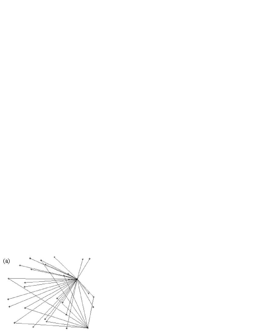
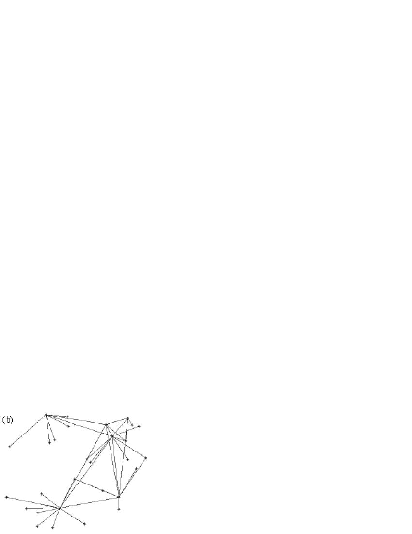
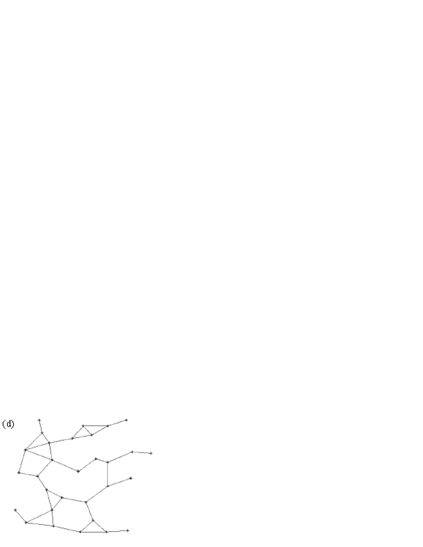
Figure 3: Four networks with different topology are shown which is controlled by the parameters $\alpha$ and $\gamma$. (a) $\alpha$ takes any value and while $\gamma$=0. The network is dominated by two large hubs when $\gamma$=0; (b) $\alpha=1$ and $\gamma=1$. With the increasing of $\gamma$, the hubs become much smaller than figure (a); (c) $\alpha$ = 1 and $\gamma$ = 2; (d) $\alpha$ = 0, $\gamma$ takes any value. The topologies are strongly reminiscent of airlines and roads, respectively.

For Fig.3(a), the value of $\gamma$ = 0 makes the network only rely on the heterogeneous strength of nodes, This causes the topology is dominated by two hubs since the nodes of great heterogeneous strength is easy to magnetize others. Whereas with the $\gamma$ increasing, more effect of the geographic factor makes the node tend to connect to the closer ones and weaken the hub-and -spoke effect. When $\alpha$=1 and $\gamma$=2 (Fig.3(c)), the network exhibits some features similar to the airline network. When $\alpha$=0 (Fig.3(d)), the topology is entirely constrained by the geography, which forms a two-dimensional network strongly reminiscent of roads. As we have defined in the section II, the gravitation $G_{ij}$ describes some dynamical demands or expected traffic. From the view of operator, the significance of the equation (3) is to maximize the whole expected traffic of the network which reflects the efficiency of the network. In other words, our model provides a possible way for operators to gain the highest profit. Even though a link costs much, the operators will still earn the cost and gain profit in short order as long as the traffic within the link is large enough. Thus such a link will be constructed all the time. In summary, the cost is a minor factor compared to the dynamical demand and that is the reason we simplify the cost.

IV Simulation for the Chinese City Airline Network

The gravitation model we proposed is used to simulate the Chinese airline network Liu . The cities are considered as the nodes of the network while the edges reflect the airlines. To reproduce the real network better, we set the number of nodes n=121 and number of links E=689. The position of each node is sited on the two-dimensional plane, as it is shown in Fig. 4. The heterogeneous strength M and the distance $D_{ij}$ are, respectively, defined as the population of the city and the Euclidean distance of city i and j. Selecting $\alpha$=1 and $\gamma\in$[1,2] Chen , they are to describe the interactions of cities. Here we set $\gamma$ = 1.5.

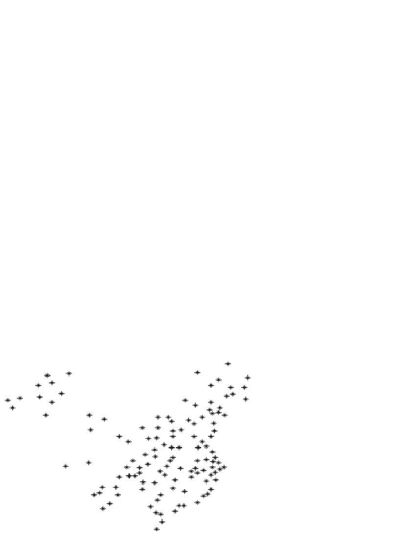
Figure 4: The geographic distribution of the cities with airports. Each city denotes a node. There are totally 121 nodes in our simulation.

Figure 5: The simulation for the Chinese airline network. Each link of two nodes reflects an airline between them. There is totally 689 links. The cities, such as Beijing, Shanghai, Guangzhou, Harbin and Urumchi, exhibit hub-and-spoke phenomenon in our simulation just as they do in the real network.

Fig. 5 shows the simulated network. Obviously, the hubs in the real network such as Beijing, Shanghai, Guangzhou, Harbin and Urumchi exhibit the similar hub-and-spoke phenomenon in our simulation. In real condition, Beijing, Shanghai and Guangzhou are the three cities with the highest degree while in our model they are, respectively, Shanghai, Beijing and Wuhan (Guangzhou is the fourth). The reason for such difference may be that using the population to denote the heterogeneous strength of city is intuitive but not be exact because the economy and the administration factors are also important indexes for the grade of city. In spite of this difference, we still succeed in reproducing the every hub and their hub-and-spoken phenomenon existing in the real network. The average shortest-path length L and degree-degree correlation exponent r of the model network are calculated, where L = 2.302, r = -0.401 while in the real network L = 2.263, r = -0.408. Fig. 6 shows the clustering-degree distribution. It meets $C(k)\sim k^{-1}$ which indicates the model network exhibits the same hierarchy as the real network does.

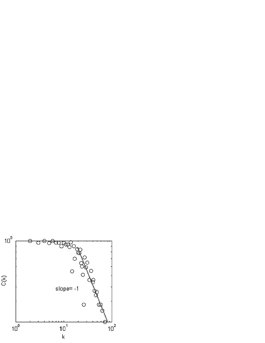
Figure 6: The clustering-degree distribution of the simulation. The distribution satisfies a linear decreasing feature with slope -1 in log-log coordinate, which indicates that the result of simulation reproduces the hierarchy.

Fig. 7 is the degree distribution of the model network.It satisfies the two-regime power-law distribution. This is an interesting result not only to verify the real degree distribution but also to produce the power-law distribution without any preferential attachment mechanism. We are not sure if it is a coincidence or caused by some other internal reasons, but we will still try to offer an explanation in the following discussion.

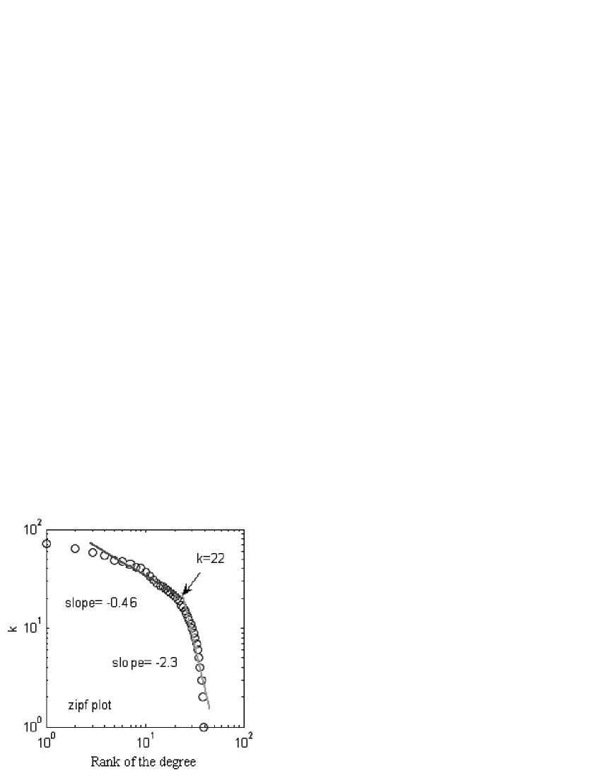
Figure 7: The degree distribution of the simulation. It presents a behavior of two-regime power-law degree distribution with the exponent$\gamma_{1}$ = -0.46 for the first power laws and $\gamma_{2}$ = -2.3 for the second. The turning point happens at degree k = 22. In comparison, $\gamma_{1}$ = -0.53, $\gamma_{2}$ = -2.05 and the turning point at degree k = 20 in the Chinese City Airline network. Both the exponents and the turning point fit the real network well.

Fig. 8 shows the correlation of the degree and node strength of our simulation. Considering the gravitation is an effective prediction of the real traffic, we let the gravitation of the two nodes represent the weight of the link between them and the node strength is the sum of such gravitation among all the links to it. As is shown in Fig. 8, the node strength increases with the degree, but does quicker than linearly, as 1.45 power, namely satisfies $S(k)\sim k^{1.45}$. This result reflected the real network well. In the Austrian airline network hdd3 and in the Chinese city airline network it indicates that node strength increases with the degree in a non-linearly manner.

Figure 8: The correlation of the degree and node strength follows $S(k)\sim k^{1.45}$, indicating the non-linearly correlation.

V More discussions about the heterogeneous nodes

As we have discussed in section II, the nodes of many real networks are usually heterogeneous. But one may ask if it is necessary or meaningful to take this factor into consideration. We argue the heterogeneity of nodes may be the key reason causing the topology that we observed in many networks. Some clues are gotten from Fig. 1.The population of the city obeys a two-regime power-law distribution which is similar to the degree distribution of the city airline network. This reminds us if it is the heterogeneous nodes that cause the heterogeneous networks whose degree distribution has a large variance or in other words, homogeneous nodes will hardly produce the hubs or scale-free properties. An indirect evidence is that hubs in the real network are usually those with large heterogeneous strength. If admitting the heterogeneity of nodes, some phenomena such as hubs and preferential attachment can be explained from the view of gravitation. Considering a node with large heterogeneous strength in a spatial network,it produces a larger gravitation field according to the gravitation view. For its extensive area of influence, many nodes are magnetized and connected to it. So the nodes with large heterogeneous strength usually have larger degree, which indicates the emergence of hubs. When a new vertex emerges, it is more possible to be magnetized by the nodes with large heterogeneous strength in the same way, which makes it tend to connect to these nodes (as is mentioned above, these nodes usually have larger degree). And this just causes the phenomenon of the preferential attachment observed in network’s evolvement. Now it may be understood why our model can produce the power-law distribution without the preferential attachment mechanism. Because such mechanism has been produced by gravitation although it is not introduced designedly. Constrained by the geography, nodes with small heterogeneous strength usually connect to the large ones nearby while the latter are able to link with other nodes of even larger heterogeneous strength far away and so on. It can be imagined that the network will exhibit the hierarchy by such organizational manner. Besides heterogeneity of nodes is also related to the dynamics – the traffic. As equation (2) shows, the heterogeneous strength influences the gravitation $G_{ij}$ which is considered as the expected traffic of node i and j. Although it is only a prediction of the real traffic, Fig. 8 shows that such prediction verifies the real condition. This point indicates that the heterogeneous strength of the node is possible a bridge by which we can associate the topology with the dynamics.

VI Conclusion

In this paper, link is caused by the potential dynamical demand among nodes which makes the nodes magnetize with each other and its value can be estimated by gravitation. Based on this, a new model for the spatial network is proposed. It can generate the topology of airline and road network and can behave well in simulating the real Chinese airline network. The gravitation model has its practical meaning that follows a principle of maximizing some expected benefit to construct and optimize the network. We argue that cost is a minor factor despite its impact of restriction compared with the dynamical demand of nodes. Heterogeneous nodes and gravitation view are two ideas indicated by our model. We think they are important in understanding the topology and the dynamics of the network. However, more demonstration studies are essential to support this point of view.

References

- (1) D.J. Watts and S.H. Strogatz, Nature (London) 393, 440 (1998).
- (2) A.-L. Barab si and R.Albert, Science 286, 509 (1999); A.-L. Barab si, R.Albert, and H.Jeong, Physica A 272, 173 (1999)
- (3) Ding-Ding Han, Jin-Gao Liu, Yu-Gang Ma, Xiang-Zhou Cai, Wen-Qing Shen, Chin. Phy. Lett. 21, 1855 (2004); Ding-Ding Han, Jin-Gao Liu, Yu-Gang Ma, Chin. Phy. Lett., in press (2008)
- (4) R. Pastor-Satorras, A. Vespignani, Evolution and Structure of the Internet: A Statistical Physics Approach, Cambridge University Press, Cambridge (2004).
- (5) V. Latora, M. Marchiori, Phys. Rev. E 71, 015103(R) (2005).
- (6) R. Albert, I. Albert, G.L. Nakarado, Phys. Rev. E 69, 025103(R) (2004).
- (7) F. Pitts, The Profess. Geograph. 17, 15 (2004).
- (8) R. Guimer , S. Mossa, A. Turtschi, L.A.N. Amaral, Proc. Natl. Acad. Sci. USA 102, 7794 (2005); R. Guimer , L.A.N. Amaral, Eur. Phys. J. B 38, 381 (2004).
- (9) A. Barrat, M. Barthélemy, R. Pastor-Satorras, A. Vespignani, Proc. Natl. Acad. Sci. USA 101, 3747 (2004).
- (10) D.A. Smith, M. Timberlake, Urban Stud. 32, 287 (1995).
- (11) P. Crucitti, V. Latora, S. Porta, arXiv:physics/0504163
- (12) V. Latora, M. Marchiori, Physica A 314, 109 (2002).
- (13) B. Waxman, Routing of multipoint connections, IEEE J. Selec. Areas Commun. 6, 1617 (1988).
- (14) S.-H. Yook, H. Jeong, A.-L. Barab si, Proc. Natl. Acad. Sci. USA 99, 13382 (2002).
- (15) Yan-Bo Xie, Tao Zhou, Wen-jie Bai, Guangrong Chen, Wei-Ke Xiao, and Bing-Hong Wang, Phys. Rev. E 75, 036106 (2007)
- (16) J.M. Carlson, J. Doyle, Phys. Rev. E 60, 1412 (1999).
- (17) M.T.Gastner, M.E.J Newman, Eur. Phys. J. B 49, 247-252 (2006).
- (18) M.T.Gastner, M.E.J Newman, Phys. Rev. E 74, 016117(2006).
- (19) Zhenhua Wu, Lidia A.Braunstein, Vittoria Colizza, Reuven Cohen, Shlomo Havlin, H.Eugene Stanley Phys. Rev. E 74, 056104 (2006)
- (20) P.J. Macdonald, E. Almaas, A.-L. Barab si, Europhys. Lett. 72, 308 (2005).
- (21) Hong-Kun Liu, Tao Zhou, Acta Phys. Sin. 56, 0106 (2007).
- (22) Liu J S ,Chen Y G, Scintia Geographica Sinica 20, 0528 (2000).
- (23) China City Statistical Yearbook 2003 (Beijing : China Statistics Press) p16
- (24) Ding-Ding Han, Jiang-hai Qian, Jin-Gao Liu, submitted to Physica A