A bijective proof for a theorem of Ehrhart

Abstract

We give a new proof for a theorem of Ehrhart regarding the quasi-polynomiality of the function that counts the number of integer points in the integral dilates of a rational polytope. The proof involves a geometric bijection, inclusion-exclusion, and recurrence relations, and we also prove Ehrhart reciprocity using these methods.

1 Introduction.

Enumerative combinatorics is a rich and vast area of study. Particularly interesting in this subject are families of objects parameterized by the positive integers $\mathbf{Z}_{>0}$ with an associated counting function $f(t)$ that is polynomial; this last statement means that there is some polynomial $p(t)$ such that $p(t)=f(t)$ for all $t\in\mathbf{Z}_{>0}$.

It is a bit mysterious that polynomial sequences arise at all in enumerative combinatorics. Even more so, these polynomials should a priori have no meaning when evaluated at negative values. However, the surprising fact is that they oftentimes do; such occurrences are usually called combinatorial reciprocity theorems. To warm up, we will begin with two examples of combinatorial reciprocity theorems related to finite graphs and partially ordered sets (posets, for short). The main subject of this paper will be a combinatorial reciprocity theorem related to counting lattice points in polytopes. To motivate this topic, we will discuss Pick’s theorem shortly, which is a special case of the reciprocity theorem in dimension 2.

For the first example, let $\Gamma$ be a finite undirected graph with $n$ vertices, and let $V(\Gamma)$ denote its vertex set. For $t\in\mathbf{Z}_{>0}$, a $t$-coloring of $\Gamma$ is a function $c\colon V(\Gamma)\to\{1,\dots,t\}$. A $t$-coloring is proper if $c(v)\neq c(v^{\prime})$ whenever $v$ and $v^{\prime}$ are adjacent vertices. The function $\chi_{\Gamma}(t)$ which counts the number of proper $t$-colorings of $\Gamma$ is a polynomial of degree $n$ called the chromatic polynomial of $\Gamma$. Surprisingly, there is a nice combinatorial interpretation for the number $(-1)^{n}\chi_{\Gamma}(-t)$ for $t\in\mathbf{Z}_{>0}$. First, some more definitions. Given an orientation of the edges of $\Gamma$, a directed cycle is a sequence of vertices $(v_{0},\dots,v_{r})$ such that there is an edge oriented from $v_{i-1}$ to $v_{i}$ for $i=1,\dots,r$ and $v_{0}=v_{r}$. An orientation of $\Gamma$ is acyclic if it has no directed cycles. We say that a $t$-coloring is compatible with an orientation of $\Gamma$ if for every edge oriented from vertex $v_{1}$ to $v_{2}$, $c(v_{1})\leq c(v_{2})$. Then $(-1)^{n}\chi_{\Gamma}(-t)$ is the number of pairs $(\alpha,c)$ where $\alpha$ is an acyclic orientation of $\Gamma$ and $c$ is $t$-coloring compatible with $\alpha$. By convention, if $\Gamma$ has no edges, there is exactly one orientation on the edges of $\Gamma$. In particular, $(-1)^{n}\chi_{\Gamma}(-1)$ counts the number of acyclic orientations of $\Gamma$.

For the next example, let $P$ be a finite poset with $n$ elements. The function $\Omega_{P}(t)$ which counts the number of order-preserving maps $\varphi\colon P\to\{1,\dots,t\}$, i.e., maps with the property that if $x\leq y$ for $x,y\in P$, then $\varphi(x)\leq\varphi(y)$, is a polynomial called the order polynomial of $P$. The combinatorial reciprocity theorem in the example of the order polynomial $\Omega_{P}(t)$ is much simpler: $(-1)^{n}\Omega_{P}(-t)$ is the number of strict order-preserving maps $\varphi\colon P\to\{1,\dots,t\}$, i.e., maps with the property that if $x<y$ for $x,y\in P$, then $\varphi(x)<\varphi(y)$.

These interpretations are indeed a bit unexpected, but in the author’s opinion, this is one of the more attractive features of mathematics.

In this paper we will discuss another instance of combinatorial reciprocity that is related to a famous theorem proven by Georg Pick. Pick led a productive mathematical life and worked in many different fields ranging from functional analysis and linear algebra to complex analysis and differential geometry. His most famous result now is Theorem 1, commonly known as Pick’s theorem. When first published, Pick’s theorem did not receive much attention. It was, however, included in the famous book Mathematical Snapshots [17] which was first published in 1969, and it then attracted much more attention. During World War II, Pick was sent to the Theresienstadt concentration camp in 1942 and died there shortly after that. More information on Pick’s life can be found at http://www-history.mcs.st-and.ac.uk/Biographies/Pick.html.

Before stating Pick’s theorem, we need a bit of notaton. Let ${\mathcal{P}}$ be a connected and simply connected polygon (not necessarily convex, but we do assume our polygons are simple) in the plane whose vertices lie in $\mathbf{Z}^{2}$. For the rest of this paper, elements of $\mathbf{Z}^{2}$, and, more generally, $\mathbf{Z}^{n}$, will be referred to as integer points, integral points, and sometimes lattice points. Let $A$ be the area of ${\mathcal{P}}$, let $B$ be the number of integer points on the boundary of ${\mathcal{P}}$, and let $I$ be the number of integer points in the interior of ${\mathcal{P}}$. Pick’s famous theorem [12] (also see [1, Theorem 2.8] for a modern treatment) relates these quantities:

Theorem 1 (Pick).

Let ${\mathcal{P}}$ be a connected and simply connected polygon in the plane whose vertices lie in $\mathbf{Z}^{2}$. With the notation above,

$$A=I+\frac{B}{2}-1.$$ (1)

Now let $t$ be a positive integer; we consider dilates $t{\mathcal{P}}:=\{tx\mid x\in{\mathcal{P}}\}$. The area of $t{\mathcal{P}}$ is $At^{2}$ and the number of integer points on the boundary of ${\mathcal{P}}$ is $Bt$. If we let $I(t)$ denote the number of integer points in the interior of $t{\mathcal{P}}$, then (1) becomes

$$At^{2}=I(t)+\frac{B}{2}t-1.$$ (2)

We know that the number of integer points of $t{\mathcal{P}}$ is $I(t)+Bt$, so by adding $\frac{B}{2}t+1$ to both sides of (2), we find that the total number of integer points $L_{\mathcal{P}}(t)$ of $t{\mathcal{P}}$ is

$$L_{\mathcal{P}}(t)=At^{2}+\frac{B}{2}t+1.$$

The right-hand side is a quadratic polynomial in $t$. Let $L_{{\mathcal{P}}^{\circ}}(t)$ denote the number of interior integer points of $t{\mathcal{P}}$. The important observation is that

$$L_{{\mathcal{P}}^{\circ}}(t)=At^{2}-\frac{B}{2}t+1,$$

which leads to the functional equation

$$L_{{\mathcal{P}}^{\circ}}(t)=L_{\mathcal{P}}(-t).$$ (3)

All of this can be illustrated by counting integer points in Figure 1.

Figure 1: An example of an integral polygon.

This can, and will, be generalized to higher dimensions. However, a bit should be said about how one might generalize Pick’s theorem. For example, can one compute the volume of a 3-dimensonal polyhedron by counting its integer points? The answer is no, and comes in the form of an example:

Example 2.

Let $T_{h}$ be the tetrahedron whose vertices are the points $(0,0,0)$, $(1,0,0)$, $(0,1,0)$, and $(1,1,h)$ for $h\in\mathbf{Z}_{>0}$; its base is the triangle whose vertices are the first three points mentioned. The volume of $T_{h}$ is $\frac{1}{3}$ times the area of the base times the height, which is $h$. This comes out to $\frac{h}{6}$. It is not hard to see that the only integer points inside of $T_{h}$ are the four points mentioned above: a general point $P\in T_{h}$ looks like

$$P=a(0,0,0)+b(1,0,0)+c(0,1,0)+d(1,1,h)$$

where $a,b,c,d\geq 0$ and $a+b+c+d=1$. Then if $P\in\mathbf{Z}^{3}$, we have to have $b,c,d\in\{0,1\}$. But if any of them is 1, then the other three coefficients must be 0, and if they are all 0, then $P$ is the origin. So we are left with the fact that $T_{h}$ always has 4 integer points but the volume grows arbitrarily large as $h$ tends to infinity. Thus, no higher-dimensional analogue of Pick’s theorem can hold.

It is worth mentioning that this example was first used by John Reeve in 1957 (see [14]) to show that the idea of computing area from counting integer points does not generalize to 3 dimensions. For the reader who comes back to this example, its Ehrhart polynomial is

$$L_{T_{h}}(t)=\frac{h}{6}t^{3}+t^{2}+\left(2-\frac{h}{6}\right)t+1,$$

so $T_{13}$ has negative coefficients in its Ehrhart polynomial.

Nevertheless, there is a theorem (Theorem 4), now called Ehrhart’s theorem, which is, in a vague sense, the correct way to generalize Pick’s theorem to higher dimensions. It was proven by Eugène Ehrhart, who was not a professional mathematician. He spent most of his life teaching mathematics in high schools in France and did his research on the side as a hobby. He proved his eponymous theorem in 1962 [6], and it wasn’t until the age of 60 that he obtained his Ph.D. with his thesis, Sur un problème de géométrie diophantienne linéaire (On a linear problem in Diophantine geometry). Most of his papers concern discrete geometry and Diophantine equations. For more information about Ehrhart, the reader might see the website http://icps.u-strasbg.fr/~clauss/Ehrhart.html.

In this paper, we are interested in the Ehrhart polynomial of an integral polytope. In Section 5, we shall be interested in the Ehrhart quasi-polynomial of a rational polytope. Though we haven’t defined these terms yet, what’s to come should be clear: we will construct a counting function associated to an integral polytope, show that it agrees with a polynomial for positive integers (in fact also for 0), and then derive a combinatorial reciprocity theorem. While the theorems are originally due to Ehrhart [6] and Macdonald [9], our proof is new. In particular, our proof of Ehrhart–Macdonald reciprocity clears up some of the mystery (see Figure 4) of its statement. While the conceptual idea of the proof is simple, verifying the details involves many manipulations of summations, which can be a bit exhausting. To remedy this, we have provided general ideas of how the proofs are to work through examples before each proof.

Before proceeding, we should mention that the first two examples presented in the introduction are special cases of Ehrhart’s theorem, because one can translate problems about counting proper colorings or order preserving maps into counting integer points in some integral polytope (or at least something approximately equal to an integral polytope for which Ehrhart’s theorem is true). For the connection between chromatic polynomials (and more) and counting integer points, the reader is encouraged to read [3], and for the connection with order polynomials, the article [16] is recommended.

2 Statements of results.

We will now give some definitions and explain the general setup. Given points $p_{1},\dots,p_{n}\in\mathbf{R}^{n}$, a convex combination of $p_{1},\dots,p_{n}$ is a linear combination $a_{1}v_{1}+\cdots+a_{n}v_{n}$ where $a_{i}\geq 0$ for $i=1,\dots,n$ and $a_{1}+\cdots+a_{n}=1$. The convex hull of a set $S\subseteq\mathbf{R}^{n}$ is the set of all convex combinations of $S$:

$$\operatorname*{conv}(S):=\{a_{1}x_{1}+\cdots+a_{r}x_{r}\mid a_{i}\geq 0,\ a_{1}+\cdots+a_{r}=1,\ x_{i}\in S\}.$$

Another equivalent definition is that the convex hull of $S$ is the intersection of all convex sets containing $S$; we’ll be more interested in the first definition. An integral (respectively, rational) polytope ${\mathcal{P}}\subset\mathbf{R}^{n}$ is the convex hull of finitely many integral (respectively, rational) points in $\mathbf{R}^{n}$. The dimension of ${\mathcal{P}}$ is the dimension of its affine span (or, equivalently, one could translate some point in ${\mathcal{P}}$ to the origin and compute the dimension of the vector subspace of $\mathbf{R}^{n}$ that its points generate). If $v\in{\mathcal{P}}$ cannot be written as a convex combination of any subset of points in ${\mathcal{P}}$ that does not include $v$, then $v$ is a vertex of ${\mathcal{P}}$. In particular, ${\mathcal{P}}$ is the convex hull of its vertices, and there are only finitely many of them. If the dimension of ${\mathcal{P}}$ is $d$, and ${\mathcal{P}}$ has $d+1$ vertices, we say that ${\mathcal{P}}$ is a simplex. Note that by linear independence, the representation of a point inside of a simplex as a convex combination of its vertices is necessarily unique. Let ${\mathcal{P}}^{\circ}$ denote the relative interior of ${\mathcal{P}}$, i.e., the topological interior of ${\mathcal{P}}$ in its affine span with the subspace topology. It is not hard to see that the relative interior of a simplex with vertices $v_{0},\dots,v_{d}$ is the set of convex combinations $a_{0}v_{0}+\cdots+a_{d}v_{d}$ where $a_{i}>0$ for $i=0,\dots,d$.

Given a polytope ${\mathcal{P}}$, we define a scalar multiplication $t{\mathcal{P}}:=\{tx\mid x\in{\mathcal{P}}\}$ for $t\in\mathbf{R}$, but we shall restrict our attention to $t\in\mathbf{Z}$. Now define $\ell_{\mathcal{P}}\colon\mathbf{Z}\to\mathbf{Z}_{\geq 0}$ by

$$\ell_{\mathcal{P}}(t):=\begin{cases}\#(t{\mathcal{P}}\cap\mathbf{Z}^{n})&\text{if }t>0,\\ 1&\text{if }t=0,\\ (-1)^{\dim{\mathcal{P}}}\#(t{\mathcal{P}}^{\circ}\cap\mathbf{Z}^{n})&\text{if }t<0.\end{cases}$$

Here $\#$ denotes the cardinality of a set. This definition may seem strange, but now the goal of this paper becomes easy to state:

Theorem 3 (Ehrhart, Macdonald).

If ${\mathcal{P}}\subset\mathbf{R}^{n}$ is an integral polytope of dimension $d$, then there exists a polynomial $L_{\mathcal{P}}(t)$ of degree $d$ such that $L_{\mathcal{P}}(t)=\ell_{\mathcal{P}}(t)$ for all $t\in\mathbf{Z}$.

Unfolding this compact statement, we obtain the following two theorems.

Theorem 4 (Ehrhart).

If ${\mathcal{P}}\subset\mathbf{R}^{n}$ is an integral polytope of dimension $d$, then the function $\#(t{\mathcal{P}}\cap\mathbf{Z}^{n})$ agrees with a polynomial $L_{\mathcal{P}}(t)$ of degree $d$ for all nonnegative integers.

The polynomial $L_{\mathcal{P}}(t)$ is called the Ehrhart polynomial of ${\mathcal{P}}$. The combinatorial reciprocity theorem associated with it is the following statement.

Theorem 5 (Ehrhart–Macdonald reciprocity).

If ${\mathcal{P}}\subset\mathbf{R}^{n}$ is an integral polytope of dimension $d$, then for $t\in\mathbf{Z}_{>0}$,

$$(-1)^{d}L_{{\mathcal{P}}}(-t)=\#(t{\mathcal{P}}^{\circ}\cap\mathbf{Z}^{n}).$$

Compare this with (3). Our proof of these theorems uses the following standard result [15, Corollary 4.3.1].

Lemma 6.

For $f\colon\mathbf{Z}_{\geq 0}\to\mathbf{C}$ and $d\in\mathbf{Z}_{\geq 0}$, the following are equivalent:

1. There exists $P(z)\in\mathbf{C}[z]$ with $\deg P\leq d$ such that

   $$\sum_{t\geq 0}f(t)z^{t}=\frac{P(z)}{(1-z)^{d+1}}\,.$$

2. For all $t\geq 0$,

   $$\sum_{k=0}^{d+1}(-1)^{d+1-k}\binom{d+1}{k}f(t+k)=0.$$

3. There is a polynomial of degree $\leq d$ that agrees with $f(t)$ for all nonnegative integers.

The original proof of Theorem 4 by Ehrhart [6] uses the equivalence of items (i) and (iii) from Lemma 6, but we shall make use of the equivalence of items (ii) and (iii). For another account of Ehrhart’s proof, the book [1] is recommended. A completely different approach using the machinery of toric varieties can be found in [11, Chapter 13]. We should mention that though the algebro-geometric proof of Ehrhart’s theorem uses much more machinery than may seem necessary, it does have the nice feature that it does not appeal to triangulations to reduce to the case that the polytope is a simplex. Going back to our proof, since the equivalence of items (ii) and (iii) is so crucial to our approach, we will give a proof.

Proof of equivalence of items (ii) and (iii) of Lemma 6.

The proof is by induction on $d$. If $d=0$, then the equivalence says that $f$ is a constant function if and only if $f(t+1)-f(t)=0$ for all $t$, which is clear. Now suppose that $d>0$, and assume that the equivalence holds for $d-1$.

Suppose that (iii) holds. Then $g(t)=f(t+1)-f(t)$ is a polynomial of degree $\leq d-1$, so by the inductive hypothesis,

$$0 =\sum_{k=0}^{d}(-1)^{d-k}\binom{d}{k}(f(t+1+k)-f(t+k))$$

$$=\sum_{k=1}^{d+1}(-1)^{d-k+1}\binom{d}{k-1}f(t+k)+\sum_{k=0}^{d}(-1)^{d-k+1}\binom{d}{k}f(t+k)$$

$$=f(t+d+1)+(-1)^{d+1}f(t)+\sum_{k=1}^{d}(-1)^{d-k+1}\binom{d+1}{k}f(t+k)$$

$$=\sum_{k=0}^{d+1}(-1)^{d-k+1}\binom{d+1}{k}f(t+k).$$

Now suppose that (ii) holds. Running backwards through the above calculations, we see that the function $g(t)=f(t+1)-f(t)$ satisfies (ii) for $d-1$ instead of $d$, so by the inductive hypothesis, there is a polynomial of degree $\leq d-1$ that agrees with $g(t)$ for all nonnegative integers. Then we can write $f(t+1)=g(t)+f(t)$, and by induction on $t$ this becomes

$$f(t+1)=f(0)+\sum_{k=0}^{t}g(k).$$

So it is enough to check that the sum on the right is a polynomial. By breaking $g$ up into monomials, we can reduce to showing that $\sum_{k=0}^{t}k^{r}$ is a polynomial. This is a well-known fact, but here is a short proof. Since $t^{r}$ is a rational polynomial, it is in the rational vector space with basis $\binom{t}{i}$ for $i\in\mathbf{N}$. So we can make the further reduction of showing that $\sum_{k=0}^{t}\binom{k}{i}$ is a polynomial for fixed $i$. But this is true because of the identity

$$\sum_{k=0}^{t}\binom{k}{i}=\binom{t+1}{i+1}.$$

To see why this identity holds, note that the right-hand side counts $(i+1)$-subsets of $\{1,\dots,t+1\}$, while the left-hand side counts the same thing if we interpret each $\binom{k}{i}$ as counting the number of $(i+1)$-subsets of $\{1,\dots,k+1\}$ which contain $k+1$. ∎

3 The Ehrhart polynomial of an integral polytope.

To get a feel for the geometric idea behind the proof of Theorem 4, we begin by considering the polytope ${\mathcal{P}}$ whose vertices are $(0,0)$, $(2,0)$, and $(2,1)$. The large triangle in Figures 2 and 3 is $3{\mathcal{P}}$, and the shaded subtriangles display the following recurrence relation:

$$\ell_{\mathcal{P}}(3)=3\ell_{\mathcal{P}}(2)-3\ell_{\mathcal{P}}(1)+\ell_{\mathcal{P}}(0).$$

Proof of Theorem 4.

We will show that

$$\ell_{{\mathcal{P}}}(t+d+1)=\sum_{k=0}^{d}(-1)^{d-k}\binom{d+1}{k}\ell_{{\mathcal{P}}}(t+k)$$ (4)

for all $t\geq 0$; then Lemma 6 gives the polynomiality of the sequence $\ell_{{\mathcal{P}}}(t)$. It is sufficient to prove (4) for simplices because any integral polytope ${\mathcal{P}}$ can be triangulated into simplices $\{T_{i}\}$ such that each vertex of each $T_{i}$ is a vertex of ${\mathcal{P}}$ (a proof of this can be found in [1, Appendix B]). Inclusion-exclusion then gives $\ell_{{\mathcal{P}}}(t)$ as a sum of the $\ell_{T_{i}}(t)$ with appropriate signs. So without loss of generality, we may assume that ${\mathcal{P}}$ is a simplex.

Let $\{v_{0},\dots,v_{d}\}$ be the vertices of ${\mathcal{P}}$ and fix an integer $t\geq 0$. For each vertex $v_{i}$ of ${\mathcal{P}}$, define $Q_{i}:=(t+d){\mathcal{P}}+v_{i}$. See Figure 2 for an example where $d=2$, $t=0$, and ${\mathcal{P}}$ is the convex hull of $\{(0,0),(2,0),(2,1)\}$.

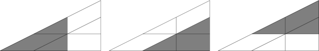
Figure 2: From left to right: $Q_{0},Q_{1},Q_{2}$

We use inclusion-exclusion to compute the number of integer points in $Q:=\bigcup_{i}Q_{i}$. That is, we add the number of integer points that are contained in each $Q_{i}$, subtract those that are contained in each intersection of two $Q_{i}$, etc. By our construction of these simplices, we can describe the $k$-fold intersections explicitly. For our running example, see Figure 3.

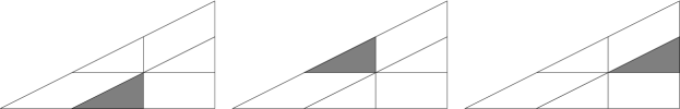
Figure 3: From left to right: $Q_{0}\cap Q_{1},Q_{0}\cap Q_{2},Q_{1}\cap Q_{2}$.

The first observation is that

$$Q_{j} =(t+d){\mathcal{P}}+v_{j}$$

$$=\left\{v_{j}+\sum_{i=0}^{d}(t+d)c_{i}v_{i}\ \middle|\ c_{i}\geq 0,\sum_{i=0}^{d}c_{i}=1\right\}$$

$$=\left\{\sum_{i=0}^{d}a_{i}v_{i}\ \middle|\ a_{j}\geq 1,a_{i}\geq 0\text{ if }i\neq j,\text{ and }\sum_{i=0}^{d}a_{i}=t+d+1\right\},$$

so for any $I\subseteq D:=\{0,\dots,d\}$,

$$\bigcap_{i\in I}Q_{i} =\left\{\sum_{i=0}^{d}a_{i}v_{i}\ \middle|\ a_{i}\geq 1\text{ if }i\in I,a_{i}\geq 0\text{ if }i\notin I,\text{ and }\sum_{i=0}^{d}a_{i}=t+d+1\right\}$$

$$=(t+d+1-\#I){\mathcal{P}}+\sum_{i\in I}v_{i}.$$

For each $k=1,\dots,d+1$, there are $\binom{d+1}{d+1-k}$ $k$-fold intersections, and each contains $\ell_{\mathcal{P}}(t+d+1-k)$ integer points because the sets differ from one another by an integer translate. So inclusion-exclusion gives

$$\#(Q\cap\mathbf{Z}^{n}) =\sum_{k=1}^{d+1}(-1)^{k+1}\sum_{\begin{subarray}{c}I\subseteq D\\ \#I=k\end{subarray}}\#\left(\bigcap_{i\in I}Q_{i}\cap\mathbf{Z}^{n}\right)$$

$$=\sum_{k=1}^{d+1}(-1)^{k+1}\binom{d+1}{d+1-k}\ell_{{\mathcal{P}}}(t+d+1-k)$$

$$=\sum_{k=0}^{d}(-1)^{d-k}\binom{d+1}{k}\ell_{{\mathcal{P}}}(t+k).$$

Note that if $t=k=0$, then our definition $\ell_{\mathcal{P}}(0)=1$ coincides with the fact that the intersection of all the $Q_{j}$ is a single integer point. The right-hand side of this equation coincides with the right-hand side of (4). To finish, we show that $Q=(t+d+1){\mathcal{P}}$. It is clear that $Q\subseteq(t+d+1){\mathcal{P}}$. To prove the other inclusion, first note that

$$(t+d+1){\mathcal{P}}=\left\{\sum_{i=0}^{d}a_{i}v_{i}\ \middle|\ a_{i}\geq 0,\ \sum_{i=0}^{d}a_{i}=t+d+1\right\}.$$

Since $t\geq 0$, it follows that for any point $P=a_{0}v_{0}+\cdots+a_{d}v_{d}\in(t+d+1){\mathcal{P}}$, there must exist some $j$ such that $a_{j}\geq 1$. (This is one of the reasons why it is important that we are assuming that ${\mathcal{P}}$ is a simplex.) Then $P\in Q_{j}$, so $(t+d+1){\mathcal{P}}\subseteq Q$, and we conclude that there exists a polynomial $L_{\mathcal{P}}(t)$ such that $L_{\mathcal{P}}(t)=\#(t{\mathcal{P}}\cap\mathbf{Z}^{n})$ for $t\in\mathbf{Z}_{\geq 0}$.

Finally, we must show that the degree of the polynomial $L_{\mathcal{P}}(t)$ is $d$. The above work shows that $L_{\mathcal{P}}(t)$ is a polynomial of degree at most $d$. By translating ${\mathcal{P}}$ if necessary, we may assume that one of its vertices is the origin. Since ${\mathcal{P}}$ is $d$-dimensional, there are vertices $v_{1},\dots,v_{d}$ that are linearly independent when considered as vectors. For positive integers $k_{1},\dots,k_{d}\leq t$, the point $k_{1}v_{1}+\cdots+k_{d}v_{d}$ lives in $dt{\mathcal{P}}\cap\mathbf{Z}^{n}$, and these points are all distinct for different choices of $k_{i}$ by linear independence of the $v_{i}$. Hence $L_{\mathcal{P}}(dt)\geq t^{d}$, which shows that $L_{\mathcal{P}}(t)$ has degree at least $d$. ∎

4 Ehrhart–Macdonald reciprocity.

As in the case of the proof of Theorem 4, the idea behind the proof of Theorem 5 can be seen in Figure 4: again we are considering the polytope ${\mathcal{P}}$ whose vertices are $(0,0)$, $(2,0)$, and $(2,1)$. The figure depicts $2{\mathcal{P}}$ and illustrates the recurrence relation

$$\ell_{\mathcal{P}}(2)=3\ell_{\mathcal{P}}(1)-3\ell_{\mathcal{P}}(0)+\ell_{\mathcal{P}}(-1).$$

Proof of Theorem 5.

We first handle the case when ${\mathcal{P}}$ is a simplex. Going back to the proof of Lemma 6, it is clear that if $f\colon\mathbf{Z}_{\geq N}\to\mathbf{C}$ for some integer $N$ then the statement that item (ii) of Lemma 6 holds for all $t\geq N$ is equivalent to the statement that there exists a polynomial of degree $\leq d$ that agrees with $f(t)$ for all $t\geq N$. So to prove that there is a polynomial that agrees with $\ell_{\mathcal{P}}(t)$ for all integers, it will be enough to show that (4) holds for all integers $t$.

The content of Theorem 4 is the case $t\geq 0$. For $t\leq-d-1$, the proof is similar to the proof for Theorem 4 because every occurrence of ${\mathcal{P}}$ can be replaced by $-{\mathcal{P}}^{\circ}$, and the statements are valid after replacing weak inequalities (inside of the set descriptions of the $Q_{i}$’s and their intersections) with strict inequalities. So we may assume that $0>t>-d-1$. As before, define $Q_{i}:=(t+d){\mathcal{P}}+v_{i}$ and $Q:=\bigcup_{i}Q_{i}$. Then the equality

$$\#(Q\cap\mathbf{Z}^{n})=\sum_{k=1}^{t+d+1}(-1)^{k+1}\binom{d+1}{d+1-k}\ell_{{\mathcal{P}}}(t+d+1-k)$$ (5)

holds by the same reasoning as in the proof of Theorem 4. However, we cannot say that $(t+d+1){\mathcal{P}}=Q$. Indeed, we can describe this deficiency explicitly:

$$(t+d+1){\mathcal{P}}\setminus Q=\left\{\sum_{i=0}^{d}a_{i}v_{i}\ \middle|\ 0\leq a_{i}<1,\ \sum_{i=0}^{d}a_{i}=t+d+1\right\}.$$

See Figure 4 for an example in which $d=2$, $t=-1$, and ${\mathcal{P}}$ is the convex hull of $\{(0,0),(2,0),(2,1)\}$. In this example, note that the hole is precisely $-{\mathcal{P}}^{\circ}+(4,2)$.

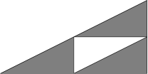
Figure 4: The deficiency $(t+d+1){\mathcal{P}}\setminus Q$.

Now define

$${\mathcal{P}}^{\prime}:=t{\mathcal{P}}^{\circ}+\sum_{i}v_{i}.$$

First note that

$$t{\mathcal{P}}^{\circ}=\left\{\sum_{i=0}^{d}a_{i}v_{i}\ \middle|\ a_{i}<0,\ \sum_{i=0}^{d}a_{i}=t\right\},$$

which implies

$${\mathcal{P}}^{\prime}=t{\mathcal{P}}^{\circ}+\sum_{i=0}^{d}v_{i}=\left\{\sum_{i=0}^{d}a_{i}v_{i}\ \middle|\ a_{i}<1,\ \sum_{i=0}^{d}a_{i}=t+d+1\right\}.$$

If $t=-1$, then ${\mathcal{P}}^{\prime}=(t+d+1){\mathcal{P}}\setminus Q$ because each coefficient $a_{i}$ needs to be nonnegative if they are to sum to $d$. Otherwise, we can try to cover ${\mathcal{P}}^{\prime}$ by simplices of the form

$$Q^{\prime}_{j}:=(t+1){\mathcal{P}}^{\circ}+\sum_{\begin{subarray}{c}i=0\\ i\neq j\end{subarray}}^{d}v_{i}$$

as in Theorem 4. Define $Q^{\prime}:=\bigcup_{i}Q^{\prime}_{i}$ for $t<-1$ and $Q^{\prime}=\varnothing$ for $t=-1$. We shall show that ${\mathcal{P}}^{\prime}\setminus Q^{\prime}=(t+d+1){\mathcal{P}}\setminus Q$. The case $t=-1$ was discussed above, so assume $t<-1$. Then

$$Q^{\prime}_{j} =(t+1){\mathcal{P}}^{\circ}+\sum_{\begin{subarray}{c}i=0\\ i\neq j\end{subarray}}^{d}v_{i}$$

$$=\left\{\sum_{i=0}^{d}a_{i}v_{i}\ \middle|\ a_{j}<0,a_{i}<1\text{ if }i\neq j,\text{ and }\sum_{i=0}^{d}a_{i}=t+d+1\right\},$$

so

$${\mathcal{P}}^{\prime}\setminus Q^{\prime}=\left\{\sum_{i=0}^{d}a_{i}v_{i}\ \middle|\ 0\leq a_{i}<1,\ \sum_{i=0}^{d}a_{i}=t+d+1\right\}=(t+d+1){\mathcal{P}}\setminus Q.$$

Inclusion-exclusion once again gives (remember what $\ell_{\mathcal{P}}(t)$ means when $t$ is negative!)

$$\#(Q^{\prime}\cap\mathbf{Z}^{n}) =\sum_{k=1}^{-(t+1)}(-1)^{k+1}\binom{d+1}{d+1-k}\#((t+k){\mathcal{P}}^{\circ}\cap\mathbf{Z}^{n})$$

$$=\sum_{k=1}^{-(t+1)}(-1)^{k+1}\binom{d+1}{d+1-k}(-1)^{d}\ell_{\mathcal{P}}(t+k).$$

This holds even for $t=-1$ because the sum on the right-hand side is empty in this case. This implies that

$$\#(({\mathcal{P}}^{\prime}\setminus Q^{\prime})\cap\mathbf{Z}^{n}) =\#({\mathcal{P}}^{\prime}\cap\mathbf{Z}^{n})-\#(Q^{\prime}\cap\mathbf{Z}^{n})$$

$$=\sum_{k=0}^{-(t+1)}(-1)^{k+d}\binom{d+1}{d+1-k}\ell_{\mathcal{P}}(t+k).$$ (6)

Finally, since we know that $(t+d+1){\mathcal{P}}\setminus Q={\mathcal{P}}^{\prime}\setminus Q^{\prime}$, we can write $(t+d+1){\mathcal{P}}$ as the disjoint union of $Q$ and ${\mathcal{P}}^{\prime}\setminus Q^{\prime}$. Therefore, combining (5) and (4),

$$\ell_{\mathcal{P}}(t+d+1) =\#((t+d+1){\mathcal{P}}\cap\mathbf{Z}^{n})$$

$$=\#(Q\cap\mathbf{Z}^{n})+\#(({\mathcal{P}}^{\prime}\setminus Q^{\prime})\cap\mathbf{Z}^{n})$$

$$=\sum_{k=1}^{t+d+1}(-1)^{k+1}\binom{d+1}{d+1-k}\ell_{\mathcal{P}}(t+d+1-k)+\sum_{k=0}^{-(t+1)}(-1)^{k+d}\binom{d+1}{d+1-k}\ell_{\mathcal{P}}(t+k)$$

$$=\sum_{k=-t}^{d}(-1)^{d-k}\binom{d+1}{k}\ell_{\mathcal{P}}(t+k)+\sum_{k=0}^{-(t+1)}(-1)^{k+d}\binom{d+1}{k}\ell_{\mathcal{P}}(t+k)$$

$$=\sum_{k=0}^{d}(-1)^{d-k}\binom{d+1}{k}\ell_{\mathcal{P}}(t+k),$$

which finishes the proof for simplices.

For the general case, let ${\mathcal{P}}$ be an integral polytope with more than $d+1$ vertices. Triangulate ${\mathcal{P}}$ using only integral vertices; call this triangulation $\mathcal{T}$. There is a natural poset structure on $\mathcal{T}$, namely $T_{i}\leq T_{j}$ if $T_{i}$ is a face of $T_{j}$. Let $L({\mathcal{P}})$ denote this poset with an additional element $\hat{1}$ such that $\hat{1}\geq T_{i}$ for all $T_{i}\in\mathcal{T}$. We finish the proof for ${\mathcal{P}}$ via the Möbius inversion formula [15, Proposition 3.7.1] on $L({\mathcal{P}})$. Fix some $t\in\mathbf{Z}_{>0}$. Define $f\colon L({\mathcal{P}})\to\mathbf{Z}_{\geq 0}$ by $f(\mathcal{F})=L_{\mathcal{F}}(t)$ where $\mathcal{F}$ is a face of $\mathcal{T}$ and $f(\hat{1})=L_{\mathcal{P}}(t)$. Also, define $g\colon L({\mathcal{P}})\to\mathbf{Z}_{\geq 0}$ by $g(\mathcal{F})=(-1)^{\dim\mathcal{F}}L_{\mathcal{F}}(-t)$ where $\mathcal{F}$ is a face of $\mathcal{T}$ and $g(\hat{1})=0$. Because every point of ${\mathcal{P}}$ lies in the relative interior of a unique face of $\mathcal{T}$, we know that

$$f(\hat{1})=\ell_{\mathcal{P}}(t)=\sum_{\mathcal{F}<\hat{1}}\#(t\mathcal{F}^{\circ}\cap\mathbf{Z}^{n})=\sum_{\mathcal{F}\leq\hat{1}}g(\mathcal{F}),$$

and by the Möbius inversion formula, this is equivalent to

$$0=g(\hat{1})=\sum_{\mathcal{F}\leq\hat{1}}\mu(\mathcal{F},\hat{1})f(\mathcal{F}),$$ (7)

where $\mu$ is the Möbius function on $L({\mathcal{P}})$. Appealing to [15, Proposition 3.8.9],

$$\mu(\mathcal{F},\hat{1})=\begin{cases}0&\text{if }\mathcal{F}\subseteq\partial{\mathcal{P}}\text{ or }\mathcal{F}=\varnothing,\\ 1&\text{if }\mathcal{F}=\hat{1},\\ (-1)^{d-\dim\mathcal{F}+1}&\text{otherwise.}\end{cases}$$

Now (7) becomes

$$0=f(\hat{1})+\sum_{\mathcal{F}\in\mathcal{T}^{\circ}}(-1)^{d-\dim\mathcal{F}+1}f(\mathcal{F}),$$

where $\mathcal{T}^{\circ}$ is the set of faces of $\mathcal{T}$ that do not lie on the boundary of ${\mathcal{P}}$. In a nicer form, this is

$$L_{\mathcal{P}}(t)=(-1)^{d}\sum_{\mathcal{F}\in\mathcal{T}^{\circ}}(-1)^{\dim\mathcal{F}}L_{\mathcal{F}}(t).$$

The functions involved are polynomials, so since they agree at all positive integers, they are equal as functions. The last step is to evaluate at $-t$:

$$L_{\mathcal{P}}(-t) =(-1)^{d}\sum_{\mathcal{F}\in\mathcal{T}^{\circ}}(-1)^{\dim\mathcal{F}}L_{\mathcal{F}}(-t)$$

$$=(-1)^{d}\sum_{\mathcal{F}\in\mathcal{T}^{\circ}}\#(t\mathcal{F}^{\circ}\cap\mathbf{Z}^{n})$$

$$=(-1)^{d}\#(t{\mathcal{P}}^{\circ}\cap\mathbf{Z}^{n}).\qed$$

5 The Ehrhart quasi-polynomial of a rational polytope.

Now that we have obtained our objective, we generalize to rational polytopes. To do so, we need some more definitions. The denominator of a rational polytope ${\mathcal{P}}$ is the smallest positive integer $D$ such that $D{\mathcal{P}}$ is an integral polytope.

A quasi-polynomial $p$ with period $s$ is a piecewise defined function

$$p(t)=p_{i}(t)\quad\text{if }t\equiv i\pmod{s},$$

where the $p_{i}$ are polynomials. The degree of $p$ is the largest degree of the $p_{i}$. Equivalently, a quasi-polynomial is a polynomial whose coefficients are periodic functions with finite period.

Corollary 7 (Ehrhart–Macdonald).

Let ${\mathcal{P}}\subset\mathbf{R}^{n}$ be a rational polytope of dimension $d$ with denominator $s$. Then $L_{{\mathcal{P}}}(t)$ is a quasi-polynomial of degree $d$ with period dividing $s$, and

$$(-1)^{d}L_{{\mathcal{P}}}(-t)=\#(t{\mathcal{P}}^{\circ}\cap\mathbf{Z}^{n})$$

for all $t\in\mathbf{Z}_{>0}$.

Proof.

Again assume ${\mathcal{P}}$ is a simplex. The only place that integrality was required in the proof of Theorem 4 is in describing the $k$-fold intersections of the $Q_{i}$. That is, we translated certain sets by integral points to get the correct set-theoretic arguments. We can do the same thing now, except that now one translates by $sv_{i}$ where $v_{i}$ is a vertex to guarantee preservation of lattice points. Thus, for each $0\leq j<s$, the sequence $(L_{{\mathcal{P}}}(ts+j))_{t\in\mathbf{Z}}$ satisfies the condition for polynomiality. The jump from simplices to polytopes is the same as before. ∎

6 Concluding remarks.

Recalling the example in the introduction on Pick’s theorem, there were interpretations for the coefficients of $L_{\mathcal{P}}(t)$ when $d=2$. A more careful estimate of $L_{\mathcal{P}}(t)$ in the proof of Theorem 4 would show that for general $d$, $L_{\mathcal{P}}(t)$ is asymptotic to $t^{d}\operatorname{vol}({\mathcal{P}})$, where $\operatorname{vol}({\mathcal{P}})$ denotes the relative volume of ${\mathcal{P}}$, which is the volume of ${\mathcal{P}}$ relative to the lattice of its affine span. Thus, the leading coefficient of $L_{\mathcal{P}}(t)$ is $\operatorname{vol}({\mathcal{P}})$. The fact that the constant coefficient is 1 follows from the fact that the Euler characteristic of a polytope is 1, and that Euler characteristic is additive with respect to inclusion-exclusion. To understand the second leading coefficient $c_{d-1}$ of $L_{\mathcal{P}}(t)$, we can use Ehrhart–Macdonald reciprocity to conclude that

$$\#(\partial{\mathcal{P}}\cap\mathbf{Z}^{n})=L_{\mathcal{P}}(1)-(-1)^{d}L_{\mathcal{P}}(-1),$$

and the leading coefficient of the right-hand side is $2c_{d-1}$. This means that $2c_{d-1}$ is the sum of the relative volumes of the facets of ${\mathcal{P}}$. With just the results in this paper, this is where we must stop. Even worse, the coefficients of Ehrhart polynomials may be negative in some cases (see Example 2), so it is not even clear what to guess the other coefficients might be telling us.

If we allow ourselves to pass to the world of algebraic geometry, then the coefficients of the Ehrhart polynomial can be expressed via intersections of Todd classes on the associated toric variety of ${\mathcal{P}}$. For more details, the reader is referred to [7, Section 5.3]. In general, however, these intersection numbers are quite difficult to compute. But with some hard work, one can understand the linear coefficient for $d=3$ in terms of Dedekind sums; this is done in [13]. This work was generalized in [5, Corollary 1], which allows one to obtain the coefficients of the other terms via Fourier analysis.

In general, it is difficult to determine the minimum period of $L_{\mathcal{P}}(t)$. Indeed, there even exist examples of nonintegral polytopes whose Ehrhart quasi-polynomial has period 1. The article [10] constructs examples for all dimensions $\geq 2$ and for arbitrary denominator. For more information, the article [2] constructs simplices whose Ehrhart quasi-polynomial has coefficient functions with prescribed minimum periods, and the article [8] offers some conjectures for why the minimum period of $L_{\mathcal{P}}(t)$ is sometimes strictly smaller than the denominator of ${\mathcal{P}}$.

Consider the following generalization of counting integer points in ${\mathcal{P}}$. Instead of counting each point as 1, we weight the points by their solid angles. Given a polytope ${\mathcal{P}}\subset\mathbf{R}^{n}$ and a point $x\in\mathbf{R}^{n}$, define the solid angle at $x$ with respect to ${\mathcal{P}}$ to be

$$\omega_{\mathcal{P}}(x):=\lim_{r\to 0}\frac{\operatorname{vol}(B_{r}(x)\cap{\mathcal{P}})}{\operatorname{vol}B_{r}(x)},$$

where $B_{r}(x)$ denotes the ball of radius $r$ centered at $x$, and $\operatorname{vol}$ denotes the usual Euclidean volume in $\mathbf{R}^{n}$. We should assume ${\mathcal{P}}$ is $n$-dimensional, otherwise this limit is always 0, which is quite boring. This ratio is eventually constant for sufficiently small $r$, so $\omega_{\mathcal{P}}(x)$ is well-defined, and we can instead ask about the solid angle enumerator

$$a_{\mathcal{P}}(t):=\sum_{x\in\mathbf{Z}^{n}}\omega_{t{\mathcal{P}}}(x).$$

Note that the sum on the right is actually finite because for $x\notin t{\mathcal{P}}$, $\omega_{t{\mathcal{P}}}(x)=0$. Going through the proof of Theorem 4, it is immediate that it generalizes to the sequence for $\{a_{\mathcal{P}}(t)\}_{t\in\mathbf{Z}_{>0}}$, so there is a polynomial $A_{\mathcal{P}}(t)$ that agrees with $a_{\mathcal{P}}(t)$ for all $t\in\mathbf{Z}_{>0}$. We call $A_{\mathcal{P}}(t)$ the solid angle polynomial of ${\mathcal{P}}$. By the way, the right way to extend this sequence to $\mathbf{Z}_{\leq 0}$ can be seen from a careful analysis of Figure 4: define

$$a_{\mathcal{P}}(-t):=(-1)^{n}\sum_{x\in\mathbf{Z}^{n}}\omega_{-t{\mathcal{P}}}(x)$$

for $t\in\mathbf{Z}_{>0}$ and $a_{\mathcal{P}}(0):=0$. We do not take $-t{\mathcal{P}}^{\circ}$ because if two simplices $\Delta_{1}$ and $\Delta_{2}$ meet in a facet of both, and we pick $x\in\Delta_{1}\cap\Delta_{2}$, then

$$\omega_{\Delta_{1}\cup\Delta_{2}}(x)=\omega_{\Delta_{1}}(x)+\omega_{\Delta_{2}}(x).$$

In other words, inclusion-exclusion is easy for solid angles because there are no overlaps! Reciprocity for solid angles tells us simply that $A_{\mathcal{P}}(t)$ is either an even or odd function depending on the parity of $n$. Of course, all of the above discussion can be extended to rational polytopes by replacing polynomials with quasi-polynomials. The theory of solid angles of polytopes is still poorly understood, and the reader is referred to [1, Chapter 11] for some open problems. The recent paper [4] extends the theory of solid angles in rational polytopes and integral dilates to solid angles in arbitrary real polytopes and real dilates using techniques from harmonic analysis.

Acknowledgements.

The author thanks Aaron Dall for helpful discussions. The author also thanks Allen Knutson, Richard Stanley, and Robin Chapman for pointing out corrections and improvements to a previous draft. Finally the author thanks Matthias Beck for help with organizational issues of this paper and two anonymous referees for helpful suggestions.

Steven V Sam
Department of Mathematics
Massachusetts Institute of Technology
Cambridge, MA 02139
ssam@mit.edu
http://www.mit.edu/~ssam

References

- [1] Matthias Beck and Sinai Robins, Computing the Continuous Discretely: Integer-Point Enumeration in Polyhedra, Undergraduate Texts in Mathematics, Springer-Verlag, New York, 2007; also available at http://math.sfsu.edu/beck/ccd.html.
- [2] Matthias Beck, Steven V. Sam, and Kevin M. Woods, Maximal periods of (Ehrhart) quasi-polynomials, J. Combin. Theory Ser. A 115 (2008), 517–525; also available at arXiv:math/0702242.
- [3] Matthias Beck and Thomas Zaslavsky, Inside-out polytopes, Adv. Math. 205 (2006), 134–162; also available at arXiv:math/0309330.
- [4] David DeSario and Sinai Robins, Generalized solid angle theory for real polytopes (to appear); also available at arXiv:0708.0042.
- [5] Ricardo Diaz and Sinai Robins, The Ehrhart polynomial of a lattice polytope, Ann. of Math. (2), 145 (1997), 503–518.
- [6] Eugène Ehrhart, Sur les polyèdres rationnels homothétiques à dimensions, C. R. Acad. Sci. Paris 254 (1962), 616–618.
- [7] William Fulton, Introduction to Toric Varieties, Annals of Mathematics Studies, vol. 31, Princeton University Press, Princeton, NJ, 1997; second printing.
- [8] Christian Haase and Tyrrell B. McAllister, Quasi-period collapse and -scissors congruence in rational polytopes (to appear); also available at arXiv:0709.4070.
- [9] Ian G. Macdonald, Polynomials associated with finite cell-complexes, J. London Math. Soc. (2) 4 (1971), 181–192.
- [10] Tyrrell B. McAllister and Kevin M. Woods, The minimum period of the Ehrhart quasi-polynomial of a rational polytope, J. Combin. Theory Ser. A 109 (2005), 345–352; also available at arXiv:math/0310255.
- [11] Mircea Mustaţă, Lecture notes on toric varieties, updated notes to Introduction to Toric Varieties by William Fulton, available at http://www.math.lsa.umich.edu/~mmustata/toric_var.html.
- [12] Georg Alexander Pick, Geometrisches zur Zahlenlehre, Sitzenber, Lotos (Prague), 19 (1899) 311–319.
- [13] James E. Pommersheim, Toric varieties, lattice points and Dedekind sums, Math. Ann. 295 (1993), 1–24.
- [14] John E. Reeve, On the volume of lattice polyhedra, Proc. London Math. Soc. (3), 7 (1957), 378–395.
- [15] Richard P. Stanley, Enumerative Combinatorics I, Cambridge Studies in Advanced Mathematics, vol. 49, Cambridge University Press, Cambridge, 1997; corrected reprint.
- [16] —, Two poset polytopes, Discrete Comput. Geom. 1 (1986), 9–23.
- [17] Hugo Steinhaus, Mathematical Snapshots, Dover Publications, New York, 1999; reprint of the third edition, Oxford University Press, 1983.