A theoretical and semiemprical correction to the long-range dispersion power law of stretched graphite
Abstract
In recent years intercalated and pillared graphitic systems have come under increasing scrutiny because of their potential for modern energy technologies. While traditional ab initio methods such as the LDA give accurate geometries for graphite they are poorer at predicting physicial properties such as cohesive energies and elastic constants perpendicular to the layers because of the strong dependence on long-range dispersion forces. ‘Stretching’ the layers via pillars or intercalation further highlights these weaknesses. We use the ideas developed by [J. F. Dobson et al, Phys. Rev. Lett. 96, 073201 (2006)] as a starting point to show that the asymptotic dependence of the cohesive energy on layer spacing in bigraphene is universal to all graphitic systems with evenly spaced layers. At spacings appropriate to intercalates, this differs from and begins to dominate the power law for dispersion that has been widely used previously. The corrected power law (and a calculated coefficient) is then unsuccesfully employed in the semiempirical approach of [M. Hasegawa and K. Nishidate, Phys. Rev. B 70, 205431 (2004)] (HN). A modified, physicially motivated semiempirical method including some effects allows the HN method to be used successfully and gives an absolute increase of about to the predicted cohesive energy, while still maintaining the correct asymptotics.
I Introduction
The graphite form of carbon is a discretely layered material. The hybridised orbitals keep the layers in a rigid hexagonal pattern while the orbitals help bind the layers. This weak interlayer binding gives graphite a small elastic constant () perpendicular to the plane which allows graphite to be ‘stretched’ by pillaring (see eg. ref. [Morishige and Hamada, 2005]) and intercalation (see eg. ref. [Boehm et al., 1994]) by other substances with potentially useful applications for Hydrogen storage and other new energy technology.
Standard density functional theory (DFT) DFT based approaches such as the LDA and GGAPerdew et al. (1996) are known (see ref. [Hasegawa and Nishidate, 2004] for a summary) to have problems predicting the interlayer binding energy and interlayer elastic constant of graphite at its experimental layer separation. This is presumed to be caused by the inability of these functionals to accurately include the long-range London dispersion forces (often denoted van der Waals forces in DFT papers, a notation we adopt to maintain consistency with other work). LDA/GGA correspondingly predict an exponentially decreasing binding energy for (where is the interlayer separation distance and is the experimental interlayer separation distance) as opposed to the correct power law behaviour.
Various authors Hasegawa and Nishidate (2004); Girifalco and Hodak (2002); Rydberg et al. (2003); Dappe et al. (2006); Ortmann et al. (2006); Hasegawa et al. (2007); Rydberg et al. (2003) have proposed corrections to the LDA/GGA results that yield an additional long-range attractive layer-layer potential of the form . By contrast Dobson, White and Rubio (DWR)Dobson et al. (2006) have shown that the asymptotic power law behaviour for bigraphene is due to its unusual bandstructure near the pointWallace (1947); Saito et al. (1998), suggesting that even these ab initio and semiempirical corrections to LDA/GGA miss some important physics.
In this work we first show that the power law is universal to many-layered graphitic systems with uniform interlayer separation, including those with an infinite number of layers such as rare gas intercalated 111It can be shown that in the case of an insulating intercalate sitting on each graphene layer that the asymptotic form of the dispersion is with unchanged from the non-intercalated but stretched bulk case. It seems highly likely that this result would be the same for a non-interacting insulating layer situated between the layers. or pillared graphite.
We then use our energy expression to calculate the correct coefficient for bulk graphite and adapt the method of Hasegawa and Nishidate (HN)Hasegawa and Nishidate (2004) to emply a corrected power law, thereby permitting empirical modelling of the non-asymptotic region when . This investigation suggests that the different power-law and coefficient could have effects on semiempirical and other methods which assume a decay of the dispersion potential but that such effect may dominate only in for .
II Asymptotic power law
The success of the random-phase approximation (RPA) in generating a correlation energy functional through the Adiabatic Connection Formula and Fluctuation-Dissipation Theorem (ACFFDT) with the correct power law for long-range dispersion forces is well studiedDob ; Pitarke and Eguiluz (1998); Dobson and Wang (1999); Furche (2001); Fuchs and Gonze (2002); Miyake et al. (2002); Gould (2003); Jung et al. (2004); Marini et al. (2006). For the case of graphene compounds, DWRDobson et al. (2006) used a long-wavelength approximation to the bare density-density response () function of graphene to prove a dispersion potential for bigraphene while also reproducing known results for other materials through the same method.
If we assume (as in DWR) that the in-plane response of a graphene plane can be approximated for low surface-parallel wavenumber () by a homogenous system of similar physics then we can write the RPA equation for the interacting density-density response () as follows:
| (1) |
where the integrals are one-dimensional and is a coupling constant to be used in the adiabatic connection formula. In the case of a layered system where each layer is highly localised in space and separated by a distance so that we may rewrite equation (1) as a tensor equation over layer indices and
| (2) |
where and () so that .
We can use the ACFFDT to write the correlation energy per layer of a two-dimensionally homogeneous system as
| (3) |
Remembering that dispersion comes entirely from inter-layer correlation effects and making use of the delta functions thus lets us calculate the energy per unit area per layer of an -layered system through
| (4) |
where
| (5) |
Due to the high level of symmetry takes the form of a Toeplitz matrix. This allows us to make use of Szegö’s Theorem (ref. [Gray, 1977] contains a good review of Szegö’s Theorem and its applications) to calculate the trace in the limit (these equations can also be obtained by Fourier methods). Defining
| (6) |
as the Fourier transform of the tensor elements of we then find
| (7) |
where .
For stretched graphitic systems the dominant energy contribution of occurs when and are small so that we can approximate the bare response by its small and expansion as calculated by DWR and Eqn. 3 of ref. [González et al., 2001] We can now write where for graphene where .
If we make changes of variables and (so that ) then we can eliminate from inside the integrals222This change of variables can also be made in the energy functional of any finite number of equally spaced graphene layers making the power-law universal for evenly spaced systems. We thus obtain the energy expression
| (8) | ||||
| (9) |
with
| (10) |
and where the second term of equation (8) arises from letting in equation (10)
Equation 8 is independent of aside from the desired term so that depends only on . For the graphitic case where we find
| (11) |
By contrast the coefficient predicted by Girifalco et alGirifalco and Hodak (2002) is which gives a potential approximately four times ( vs ) as large as that of the inverse cubic power law at the experimental interlayer spacing (equivalently this means that for ).
III Non-asymptotic behaviour
While the power law will certainly be the dominant contributor to the dispersion potential for , the intermediate-range (when ) will include a number of other correlation effects. These include the potential from the atomic polarisibilities in the direction in addition to a potential from the metallic electrons promoted from the orbitals due to layer overlap and hopping. As comes entirely from overlap of the orbitals it ought to be derivable from an analysis of the band-structure. It is expected to decay as an inverse exponential in due to localisation of the orbitals. The coefficient should be largely independent of although some electrons will be promoted to metallic and graphitic response.
With such a varied collection of correlation effects it seems unlikely that any simple ab initio method will adequately include the physics in the intermediate-range. Full RPA-ACFFDT calculations would be expected to provide a seamless potential through a wide-range of however these are extremely difficult with current numerical approaches: for example, the van der Waals energetics of the semiconducting layered boron nitride system have been described succesfully using RPA energiesMarini et al. (2006), but graphite gives convergence difficultiesRubio et al. (2007).
IV Semiempirical method
LDA calculations are expected to yield fairly accurate total energies for graphene when the interlayer spacing is compressed from its equilibrium value. Likewise the dispersion potential is expected to be accurate for layer spacing much greater than that of equilibrium. The intermediate range is more difficult to predict with neither method dealing sufficiently with the physics in that region.
The method proposed in HNHasegawa and Nishidate (2004) gives a fairly simple means (with minimal empirical contribution) of connecting the two regimes through the use of a fitting function. It is a semiempirical approach as the fitting function has its parameters chosen by matching experimental values for the lattice spacing and elastic constant . While this method predicts a reasonable value for the cohesion energy of graphite it, as with other methods, does not exhibit the correct behaviour in the tail due to the incorrect use of a type dispersion law. In order to maintain consistency with this earlier work we re-examine the major results of their paper utilising the correct dispersion law. To further maintain consistency we use the parametrisation of the LDA and GGA from the same paper.
IV.1 Semiempirical approach with pure dispersion
For our first new approach we adapt Equation 5 of HN to include the corrected form of the dispersion potential
| (12) |
where . Following HN, we use a Thomas-Fermi damping function
| (13) |
where and are free parameters. The term involving is absent due to our coefficient being sourced from a bulk rather than a sum over pairwise potentials for multiple layers. is the parametrised LDA or GGA potential taken from equation 2 of HN.
As in HN we attempted to determine and by ensuring that and where GPa, and take their experimental values (from ref. [Gauster and Fritz, 1974] for and ref. [Baskin and Meyer, 1955] for and ). Using we find that the HN fitting equations do not have a solution for the LDA or GGA. This lack of solution is not unexpected as the lack of other dispersion terms is expected to underestimate the dispersion for values of .
IV.2 Semiempirical approach with mixed and dispersion
While the term will certainly dominate over for we know that it insufficiently models the physics for , which we believe to be the cause of the fitting problems with the HN method for the semi-empirical method given in (A) above. The coefficient used in HN is derived from a coefficient calculated by Girifalco et alGirifalco and Hodak (2002) and constructed to ensure good Lennard-Jones modelling for a wide variety of graphitic systems. As such we propose to use its presumed accuracy for as a correction to our van der Waals function in order to better include the intermediate range physics.
The simplest way to do this is to assume a correction to our function of the form . The term is introduced firstly to cover the dispersion interaction due to the polarizability of the and electrons in the direction perpendicular to the graphene planes, and polarisability of the electrons parallel to the plane. These contributions to the dispersion interaction do not require long-wavelength collective electronic motions and thereforeDobson et al. (2006) are presumably describable by conventional asymptotics. These interaction are not included in our term, which is solely due to polarizability of the electrons along the graphene planes. The term also has to account for the doped, metallic nature of the graphene planes near due to overlapping of electron bands arising from the hopping of electrons from layer to layer. The corresponding attraction depends on the doping level, which decays exponentially with D. While this is not a law, it does decay faster than and hence is reasonably represented.
Accordingly we now choose so that the total van der Waals potential at the experimental lattice spacing remains the same in the two methods. This implies that
| (14) |
which is true for . This correction ensures we maintain similar behaviour while obtaining a correct power law for . The van der Waals potential now takes the form
| (15) |
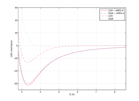
In order to ensure that equations 12-13 correctly match the empirical data we must set , for the LDA and , for the GGA when using the HN fitting function. Figure 1 shows the effect of this combined fit on both the LDA and GGA.
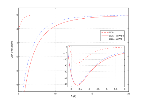
In Figure 2 we show, for the LDA case, a more detailed comparison of three methods (the LDA, that of HN and the second method proposed here). It is quite clear from the graph that the method proposed here with the extra correction closely matches that of HN for but maintains different asymptotes for . This suggests that the approximation, while a somewhat crude model of the true physics in the electron density overlap region, is able to maintain consistency with other methods.
The most ‘measurable’ effect of the semiempirical approach is the interlayer cohesive energy . Table 1 summarises the results from HN with the addition of the new results calculated here. The new power law, used as the sole dispersion term does not give a valid cohesive energy due to the lack of a solution to the fitting function for both the LDA and GGA. The effect of the correction to the van der Waals functional on the cohesive energy is to give a very close cohesive energy to those predicted by HN, differing by only for the LDA and for the GGA or about .
| LDA/GGA | Expta | Exptb | |
|---|---|---|---|
| 26.5/2.3 | |||
| L/G-vdW3 | L/G-vdW4 | L/G-vdW3+4 | |
| -/- | 60.7/57.4 | 62.4/59.7 |
V Conclusions and further work
In this paper we have investigated the asymptotic dispersion potential of ‘stretched’ graphite and found it to obey a type power law as opposed to the commonly employed . This places it in the same class of power law as bigraphene but in a different class to layered insulators ( power laws) and layered metals (). This result has important implications for semiempirical (and otherwise) corrections to the LDA/GGA which have employed an incorrect power law.
Furthermore we have employed the corrected power law in the simple semiempirical method of Hasegawa and NishidateHasegawa and Nishidate (2004) and found that, used as the sole dispersion term, it will not allow a valid solution to the HN fitting function. Reinclusion of a reduced term to include other physics from the non-asymptotic regime allows the method to be employed and gives similar results to HN for whilst ensuring the correct asymptotic behaviour is maintained. Its effect on the cohesive energy is fairly minimal with an absolute increase of the predicted cohesive energy of approximately .
While we believe that this power law (and the semi-empirical correction to it) should be accurate and useful for large layer spacings as in non-metallic intercalates and pillared systems we are not convinced that it will be as accurate in predicting the behaviour in the intermediate range of spacings without correction for other effects. Accurate RPA-ACFFDT calculations would provide a valuable benchmark for this and other methods. Until such time as these are available we hope that semi-emprical techniques like that discussed here should improve the accuracy of LDA and GGA calculations with widely spaced graphene layers.
VI Acknowledgements
The authors would like to thank Evan Gray for fruitful discussions. This research was conducted under a Discovery Grant for the Australian Research Council.
References
- Morishige and Hamada (2005) K. Morishige and T. Hamada, Langmuir 21, 6277 (2005).
- Boehm et al. (1994) H.-P. Boehm, R. Setton, and E. Stumpp, Pure and Appl. Chem. 66, 1983 (1994).
- (3) P. Hohenberg and W. Kohn. Phys. Rev. 136, B864 (1964) and W. Kohn and L. J. Sham, Phys. Rev. 140, A1133 (1965).
- Perdew et al. (1996) J. P. Perdew, K. Burke, and M. Ernzerhof, Phys. Rev. Lett. 77, 3865 (1996).
- Hasegawa and Nishidate (2004) M. Hasegawa and K. Nishidate, Phys. Rev. B 70, 205431 (2004).
- Girifalco and Hodak (2002) L. A. Girifalco and M. Hodak, Phys. Rev. B 65, 125404 (2002).
- Rydberg et al. (2003) H. Rydberg, M. Dion, N. Jacobsen, E. Schröder, P. Hyldgaard, S. I. Simak, D. C. Langreth, and B. I. Lundqvist, Phys. Rev. Lett. 91, 126402 (2003).
- Dappe et al. (2006) Y. J. Dappe, M. A. Basanta, F. Flores, and J. Ortega, Phys. Rev. B 74, 205434 (2006).
- Hasegawa et al. (2007) M. Hasegawa, K. Nishidate, and H. Iyetomi, Phys. Rev. B 76, 115424 (2007).
- Ortmann et al. (2006) F. Ortmann, F. Bechstedt, and W. G. Schmidt, Phys. Rev. B 73, 205101 (2006).
- Dobson et al. (2006) J. F. Dobson, A. White, and A. Rubio, Phys. Rev. Lett. 96, 073201 (2006).
- Wallace (1947) P. R. Wallace, Phys. Rev. B 71, 622 (1947).
- Saito et al. (1998) R. Saito, G. Dresslhaus, and M. S. Dresselhaus, Physical Properties of Carbon Nanotubes (Imperial College Press, 1998).
- Miyake et al. (2002) T. Miyake, F. Aryasetiawan, T. Kotani, M. van Schilfgaarde, M. Usuda, and K. Terakura, Phys. Rev. B 66, 245103 (2002).
- (15) J. F. Dobson, in Topics in Condensed Matter Physics, edited by M. P. Das (Nova, New York, 1994), Chap. 7: see also cond-mat 0311371.
- Pitarke and Eguiluz (1998) J. M. Pitarke and A. G. Eguiluz, Phys. Rev. B 57, 6329 (1998).
- Dobson and Wang (1999) J. F. Dobson and J. Wang, Phys. Rev. Lett. 82, 2123 (1999).
- Furche (2001) F. Furche, Phys. Rev. B 64, 195120 (2001).
- Fuchs and Gonze (2002) M. Fuchs and X. Gonze, Phys. Rev. B 65, 235109 (2002).
- Gould (2003) T. Gould, Ph.D. thesis, Griffith University (2003), URL www4.gu.edu.au:8080/adt-root/public/adt-QGU20030818.125106/in%dex.html.
- Jung et al. (2004) J. Jung, P. García-González, J. F. Dobson, and R. W. Godby, Phys. Rev. B 70, 205107 (pages 11) (2004).
- Marini et al. (2006) A. Marini, P. García-González, and A. Rubio, Phys. Rev. Lett. 96, 136404 (pages 4) (2006).
- Gray (1977) R. Gray, Toeplitz and circulant matrices: A review (1977), URL citeseer.ist.psu.edu/gray01toeplitz.html.
- González et al. (2001) J. González, F. Guinea, and M. A. H. Vozmediano, Phys. Rev. B 63, 134421 (2001).
- Rubio et al. (2007) A. Rubio, T. Miyake, and F. Aryasetiawan, Private communication (2007).
- Gauster and Fritz (1974) W. B. Gauster and I. J. Fritz, J. Appl. Phys. 45, 3309 (1974).
- Baskin and Meyer (1955) Y. Baskin and L. Meyer, Phys. Rev. 100, 544 (1955).
- Zacharia et al. (2004) R. Zacharia, H. Ulbricht, and T. Hertel, Phys. Rev. B 69, 155406 (2004).
- Benedict et al. (1998) L. X. Benedict, N. G. Chopra, M. L. Cohen, A. Zettl, S. G. Louie, and V. H. Crespi, Chem. Phys. Letters 286, 490 (1998).