Spin-Hall effects in a Josephson contact

Abstract

The Josephson tunneling through a 2D normal contact with the spin-orbit split conduction band has been studied in the diffusive regime. Linearized Usadel equations for triplet components of the pairing function revealed a striking similarity to the equations of spin diffusion driven by the electric field in normal metals. Consequently, we predict that the out-of-plane spin-Hall polarization accumulates towards lateral sample edges and the in-plane polarization is finite throughout the entire normal region. At the same time, the spin-Hall current is absent in the considered case of the stationary Josephson effect.

In connection with various spintronic applications, much interest have been attracted recently to spin-orbit interaction (SOI) effects on electron transport in normal metals and semiconductors. This interaction gives rise to fundamental transport phenomena, such as the spin-Hall effect (SHE) (for a review see Engel ) and electric spin orientation Edelstein ; Engel . These effects represent a direct manifestation of the spin-orbit coupling between spin and charge degrees of freedom in electron transport. At the same time, spin-orbit effects were also discussed for superconductors. Some works dealt with SFS junctions sfs (F stands for ferromagnet), others considered SNS sns , SN Edelstein2 systems, or bulk superconductors Edelstein2 ; Gorkov . As was pointed out in Ref. Edelstein2 ; Gorkov , SOI leads to admixture of triplet components to the pairing function. This sort of singlet-triplet coupling looks similar to the spin-charge coupling in normal systems. Therefore, one would expect that phenomena closely related to SHE could manifest themselves in superconductors. At the first sight on this problem it becomes clear that, at least in the case of zero voltage across the junction, the spin-Hall current can not be generated as a linear response to the superconducting current. The reason is that these currents have opposite parities with respect to the time inversion, while they must be equal in the stationary nondissipative superconducting transport. On the other hand, besides the spin currents, in normal systems SHE leads to spin accumulation near sample edges. Therefore, it is interesting to find out, if similar accumulation of magnetization takes place in superconducting systems. It should be noted that, despite formal similarities, such a magnetization is fundamentally distinct from that induced by the normal SHE, since it is not subject to the energy dissipation accompanying spin diffusion and relaxation in normal systems.

We will consider SHE and the electric spin orientation for a Josephson tunneling through a 2D normal contact (see Fig 1). The SOI there is represented by the Hamiltonian $H_{so}=\bm{\sigma}\cdot\mathbf{h}_{\bm{k}}$, where $\bm{\sigma}$ is a vector consisting of Pauli matrices. The spin-orbit field $\mathbf{h}_{\bm{k}}$, which is a function of the electron wave vector $\bm{k}$, can be given, for example, by Rashba RashbaSOI , or Dresselhaus Dresselhaus SOI, as well as by their combination. In this case the vector $\mathbf{h}_{\bm{k}}$ lies in the plane of the 2D system. The electron transport through the contact will be treated within the diffusion approximation, so that the length of the junction $L$, the electron coherence length $L_{c}$ and the spin precession length $L_{so}=v_{F}/h$, where $v_{F}$ is the Fermi velocity and $h$ is the angular averaged spin orbit field, are assumed to be much larger than the electron mean free path $l$. The electric voltage across the junction is set to zero. Hence, the supercurrent is provided by the phase difference between two electrodes. The analysis of such a problem will be performed within a standard semiclassical treatment of Gor’kov’s equations in the diffusion approximation (for a review see Efetov ). Our goal is to derive linearized Usadel type equations and calculate the spin density induced by SHE.

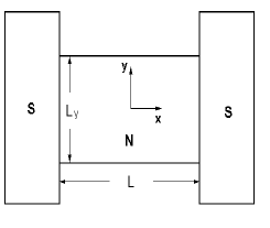
Figure 1: Josephson contact with S and N denoting superconducting and normal regions.

As far as the thermal equilibrium state is considered, all observables of interest can be expressed via retarded and advanced Green functions. The corresponding Gor’kov’s equations in the Nambu representation have the form

$$\left(i\frac{\partial}{\partial t}-\check{H}-\check{\Sigma}^{r/a}\right)\check{G}^{r/a}(X,X^{\prime})=\delta(X-X^{\prime})\,,$$ (1)

where $r$, $a$ denote retarded or advanced functions, $X=t,\mathbf{r}$ and

$$\check{H}=\frac{\tau_{3}}{2m^{*}}\hat{k}^{2}-\tau_{3}\mu+\bm{\sigma}\cdot\mathbf{h}_{\mathbf{\hat{k}}}\,,$$ (2)

with the momentum operator $\mathbf{\hat{k}}=-i\partial/\partial\bm{r}$ and the chemical potential $\mu$. After averaging of initial Green functions over random positions of short-range impurities, the self-energy in (1) takes the form agd

$$\check{\Sigma}^{r/a}(X,X^{\prime})=\frac{\tau_{3}}{2\tau\pi N_{F}}\check{G}^{r/a}(t,t^{\prime},\bm{r},\bm{r})\tau_{3}\delta(\bm{r}-\bm{r}^{\prime})\,,$$ (3)

where $\tau$ is the elastic scattering time. Unperturbed Green functions are easily obtained from Eq.(1). In the momentum representation and after the time Fourier transform they can be written as

$$\check{G}^{0r/a}(\omega,\bm{k})=\left(\omega-\tau_{3}E_{k}-\bm{\sigma}\cdot\mathbf{h}_{\bm{k}}\pm i\Gamma\right)^{-1}\,,$$ (4)

where $E_{k}=(k^{2}/2m^{*})-\mu$. Below we will perform calculations for retarded functions and drop the labels $r,a$.

Proximity to superconducting contacts results in an admixture to the Green functions of anomalous (proportional to $\tau_{1}$ and $\tau_{2}$) components. Also, these functions become inhomogeneous in space. In order to calculate them, we will follow a well known procedure in the framework of the semiclassical approximation Landau . First, we perform the Fourier transform with respect to $X-X^{\prime}$ introducing, accordingly, the frequency and wave vector variables, $\omega$ and $\bm{k}$. The center of mass variables will be remained intact and denoted as $\bm{r}$. Since the problem is stationary, the corresponding center of mass time variable is absent. Taking into account that variations of $G$ in the scale of the Fermi wave-length are small, Eq. (1) should be expanded in terms of gradients $\partial/\partial\bm{r}$. The next step is to simplify the self-energy part of Eq. (1) keeping there only terms linear in the anomalous part. Such a linearization can be done if the transparency of the SN contact is small, or the leads are close to the superconducting critical temperature. Taking the sum of Eq. (1) and its conjugate one, and making use of the fact that $\mathbf{h}_{\bm{k}}$ is an odd function of $\bm{k}$, for the anomalous part $G_{12}$ we obtain the equation

$$(2\omega-\bm{v}\cdot\mathbf{\hat{q}}+\frac{i}{\tau})G_{12} - \{\mathbf{h}_{\bm{k}}\cdot\bm{\sigma},G_{12}\}-$$

$$\frac{1}{2}\left[\delta\mathbf{h}_{\bm{k},\mathbf{\hat{q}}}\cdot\bm{\sigma},G_{12}\right] = I_{sc}\,,$$ (5)

where $\delta\mathbf{h}_{\bm{k},\mathbf{\hat{q}}}=(\mathbf{\hat{q}}\cdot\nabla_{k})\mathbf{h}_{\bm{k}}$ with $\mathbf{\hat{q}}=-i\partial/\partial\mathbf{r}$, and

$$I_{sc}=-\frac{1}{2\tau\pi N_{F}}\left(G^{0}_{11}g_{12}+g_{12}G^{0}_{22}\right)\,.$$ (6)

The lower labels in $G^{0}$ denote the matrix elements in the Nambu space and $g_{12}=\sum_{\bm{k}}G_{12}$. Usually, the quantum kinetic equation, such as (Spin-Hall effects in a Josephson contact), can be reduced to the Eilenberger Eilenberger equation by integration with respect to the electron energy. In our case this procedure is not convenient because of electron energy spin splitting. Instead, within the diffusion approximation, from Eq. (Spin-Hall effects in a Josephson contact) we will express $G_{12}$ in terms of $g_{12}$, and taking its sum over $\bm{k}$ obtain the closed diffusion equation for $g_{12}$. Before doing this, we transform the 2$\times$2 matrix $G_{12,\alpha\beta}$ to the conventional pairing function $F_{\alpha\overline{\beta}}\equiv G_{12,\alpha\beta}$, where $\overline{\beta}$ denotes the spin projection opposite to $\beta$. Further, it is convenient to decompose $F$ into triplet $F_{1},F_{-1},F_{0}$ and singlet $F_{s}$ components as

$$F_{0} = \frac{F_{12}+F_{21}}{\sqrt{2}}\,,\,\,\,\,\,F_{s}=\frac{F_{12}-F_{21}}{\sqrt{2}}$$

$$F_{1} = F_{11}\,,\,\,\,\,\,\,\,\,\,F_{-1}=F_{22}.$$ (7)

The corresponding density function $f=\sum_{\bm{k}}F$ will also be represented in a similar way. After this transformation, it is easy to see that the last term in the l.h.s. of (Spin-Hall effects in a Josephson contact) is responsible for a coupling between the singlet and triplet components of the pairing function. Besides, the singlet-triplet coupling also originates from the spin dependent parts of $G^{0}_{11}$ and $G^{0}_{22}$ in Eq. (6). Due to such coupling, the triplet component of $F$ is generated within the junction between two singlet superconductors.

For simplicity, when deriving the diffusion equation, let us assume that SOI is strong enough, so that $L_{so}\ll L_{c}$. Further, considering $I_{sc}$ together with the last term in the l.h.s. of (Spin-Hall effects in a Josephson contact) as sources, we resolve Eq.(Spin-Hall effects in a Josephson contact) performing expansion in $(\bm{v}\cdot\mathbf{\hat{q}})\tau$ and $\mathbf{h}_{\bm{k}}\tau$ up to the second order. Finally, we obtain the following diffusion equation for the triplet pairing function $f_{m}=(i/\pi N_{F})\sum_{\bm{k}}F_{m}$, $(m=0,1,-1$):

$$2i\omega f=\tau\langle\left(-i\bm{v}\cdot\frac{\partial}{\partial\bm{r}}+2\mathbf{J}\cdot\mathbf{h}_{\bm{k}}\right)^{2}\rangle f+\mathrm{M}f_{s}\,,$$ (8)

where $\mathbf{J}$ is the vector of 3$\times$3 angular moment operators and $\langle...\rangle$ denotes the angular averaging over the Fermi surface. The triplet-singlet coupling is given by

$$\mathrm{M}_{0}=0\,\,,\mathrm{M}_{\pm 1}=\frac{4\tau^{2}}{\sqrt{2}}\langle\mathrm{h}^{\mp}_{\bm{k}}(\mathbf{h}_{\bm{k}}\times\delta\mathbf{h}_{\bm{k},\mathbf{\hat{q}}})\rangle f_{s}\,,$$ (9)

with $\mathrm{h}^{\mp}_{\bm{k}}=\mathrm{h}^{x}_{\bm{k}}\mp i\mathrm{h}^{y}_{\bm{k}}$. The singlet $f_{s}$ satisfies the usual Usadel equation sfs with an additional term which is Hermitian conjugate to $M$. Since this term is small, we will neglect a corresponding correction to $f_{s}$ in Eq.(8). Hence, $f_{s}$ is given by the well known unperturbed solution in the SNS contact. Since it varies within the scale $L_{c}\gg L_{so}$, we neglected all contributions to $\mathrm{M}$ with higher powers of gradients, as well as terms proportional to $\omega\sim D/L^{2}_{c}$, where $D$ is the diffusion constant.

Without the last term in the r.h.s., Eq.(8) formally coincides with the spin diffusion equation for 2DEG in a zero electric field MalshDiff . The spin diffusion equation in the presence of the electric field has been derived in Ref. Misch for the case of the Rashba SOI, and for a general SOI in MalshAccumulation . After a linear transformation MalshDiff to spin density variables Eq.(8) will also coincide with these equations, if, apart from a constant factor, $f_{s}$ is formally identified with the electric field potential. Hence, a coupling of the spin to the electric field in normal spin transport appears to be very similar to the singlet-triplet coupling in Eq.(8).

Let us consider an example of the Rashba SOI. In this case $h^{x}_{\bm{k}}=\alpha k_{y}$ and $h^{y}_{\bm{k}}=-\alpha k_{x}$. For a homogeneous in $y$-direction case all functions depend only on $x$ and we get $f_{0}=0,f_{1}=f_{-1}$, with $f_{1}$ satisfying the equation

$$D\frac{\partial^{2}}{\partial x^{2}}f_{1}-\Gamma_{so}f_{1}=i\frac{\alpha\tau\Gamma_{so}}{\sqrt{2}}\frac{\partial}{\partial x}f_{s}\,,$$ (10)

where $\Gamma_{so}=2\tau\alpha^{2}k_{F}^{2}$ is the D’yakonov-Perel’ spin relaxation time dp . The small l.h.s. of Eq.(8) has been neglected in (10). Boundary conditions at $x=\pm L/2$ can be written in a way similar to a singlet SN interface boundary . At least in the linearized approximation the boundary conditions contain only characteristics of one-particle transmission. Therefore, they can be easily generalized to the case of a triplet pairing. Following calculations of Ref. boundary we obtain

$$(f_{1S}-gf_{1N})\big{|}_{x=\mp L/2}=\pm b\frac{\partial f_{1N}}{\partial x}\big{|}_{x=\mp L/2}\,,$$ (11)

where the labels $S$ and $N$ denote superconductor and normal sides of SN contacts at $x=\pm L/2$, and $g=|\omega|/\sqrt{(\omega+i0^{+})^{2}-|\Delta|^{2}}$ is a DOS factor for a superconductor. The characteristic length $b$ depends on the SN barrier transmittance. For our choice of parameters $b\gg L_{so}$. The same equation (11) takes place for $f_{s}$. At the low SN barrier transmission one may use the so called rigid boundary conditions and set $f_{1S}=0$. At the same time, the singlet paring function $f_{sS}|_{\mp L/2}=g\Delta\exp(\pm i\phi)/\omega$. Neglecting the third derivative of $f_{s}$, the solution of Eq. (10) can be written as

$$f_{1}=-i\frac{\alpha\tau}{\sqrt{2}}\frac{\partial}{\partial x}f_{s}+\psi(x)\,,$$ (12)

where $\psi(x)$ is a linear combination of $\exp(\pm kx)$, with $k=\sqrt{D/\Gamma}\equiv 1/L_{so}$. It is easy to see from (11) that at $kb\gg 1$ the first term dominates in Eq.(12). Therefore, $\psi$ will be neglected below.

Our next step is to calculate the spin polarization density associated with triplet components of the pairing function. This polarization is given by

$$S^{i}(\bm{r}) = \frac{i}{2}\sum_{\bm{k}}\int\frac{d\omega}{2\pi}n_{F}(\omega)\times$$ (13)

$$Tr[\sigma^{i}(G^{r}_{\bm{k}11}(\omega,\bm{r})-G^{a}_{\bm{k}11}(\omega,\bm{r})]\,,$$

where $n_{F}$ is the equilibrium Fermi distribution function. It is easy to see that the nonzero value of Eq. (13) is provided by triplet components of anomalous Green functions which contribute to $G_{11}$ with a correction term $\propto f^{2}$. Up to the leading second order with respect to $f_{s}$ and keeping only the linear terms of the triplet $f_{m}$ $(m=1,-1,0)$, for the retarded function we obtain from Eqs. (1-4)

$$\sum_{\bm{k}}Tr[\sigma^{i}G_{\bm{k}11}^{r/a}] = \frac{\mp 1}{\pi N_{F}}[\frac{i\delta^{iz}}{2}(f_{0}^{r/a}f^{+r/a}_{s}-f_{s}^{r/a}f_{0}^{+r/a})+$$ (14)

$$\frac{1}{\sqrt{2}}(f_{i}^{r/a}f^{+r/a}_{s}+f_{s}^{r/a}f_{i}^{+r/a})]\,,$$

where $f_{y}=(f_{1}+f_{-1})/2$ and $f_{x}=-i(f_{1}-f_{-1})/2$. The conjugate functions $f^{+}(\omega)=-f^{*}(-\omega)$.

In the case of Rashba SOI $f_{x}=f_{0}=0$ and $f_{y}=f_{1}$. The latter is given by Eq. (12). Then, from (14) it immediately follows that only the $y$-projection of the spin density is finite. Using the relations $f^{a}_{s}(\omega)=f^{r}_{s}(-\omega)$ and $f^{a}_{m}(\omega)=-f^{r}_{m}(-\omega)$ $(m=1,-1,0)$, we arrive to the spin polarization

$$S^{y}(x)=eN_{F}\alpha\tau\frac{J(x)}{\sigma_{dc}}\,,$$ (15)

where $\sigma_{dc}$ is the dc conductivity of the normal metal and $J$ is the Josephson current density

$$J=\frac{eD}{4\pi^{2}N_{F}}\int d\omega n_{F}(\omega)[(f_{s}^{r}\frac{\partial f^{+r}_{s}}{\partial x}-\frac{\partial f^{r}_{s}}{\partial x}f_{s}^{+r})-(r\rightleftarrows a)]\,.$$ (16)

The spin polarization (15) coincides with polarization induced in normal metals by the electric field $E$ Edelstein , if the Josephson current is substituted for the normal dissipative dc current $J_{dc}=\sigma_{dc}E$. It is easy to check that this analogy takes place also for the Dresselhaus SOI, with a little more complicated expression for $S^{i}(x)$ MalshAccumulation . An important distinction from the electric spin orientation in normal metals is that due to the charge neutrality, $J_{dc}=const$ in the $x$ direction, while the supercurrent varies inside the contact. Similar effect has been predicted by Edelstein Edelstein2 for bulk superconductors and at NS boundary, providing the supercurrent flows along the SN interface.

Let us now check, if the analogy with the electric spin orientation extends to the spin-Hall effect. Hence, our goal is to calculate $J^{z}_{y}$, which is the $y$ projection of a spin flux polarized in the $z$-direction. The corresponding spin current operator can be written as $\mathrm{J}^{z}_{y}=\{\sigma_{z},\mathrm{v}_{y}\}/2$, where the velocity $\mathrm{v}_{y}=k_{y}/m^{*}+\partial(\bm{\sigma}\cdot\bm{h}_{\bm{k}})/\partial k_{y}$. Since it has been assumed that $h_{z}=0$, one gets $\mathrm{J}^{z}_{y}=\sigma_{z}k_{y}/m^{*}$. The spin-Hall current $J_{sH}$, in its turn, can be derived from Eq.(13), with $\sigma^{i}$ substituted for $\mathrm{J}^{z}_{y}$. Keeping the same leading terms as in calculation of the spin density, we arrive to $J_{sH}=0$. This result does not depend on whether $\bm{h}_{\bm{k}}$ is given by the Rashba or Dresselhaus interactions. That is very distinct from the normal spin-Hall effect, where in the diffusive regime the spin-Hall conductance is zero for the Rashba SOI, but finite for the cubic Dresselhaus interaction MalshDress . In general, as it was discussed above, the zero value of $J_{sH}$ in superconducting transport follows from the time inversion symmetry.

Besides $J_{sH}$, in normal systems the DC current together with SOI gives rise to accumulation of the $z$-component of spin at the lateral edges of the sample MalshAccumulation ; accumulation ; Bleibaum . In the case of the Josephson junction the $z$-projection of the spin density is given by Eq.(13) and the first term in Eq. (14). Hence, it is proportional to the $f_{0}$ component of the pairing function which, in its turn, can be found from Eq.(8). For simplicity, let us consider hard wall boundaries of 2DEG at $y=\pm L_{y}/2$. In this case one can borrow the boundary conditions for Eq. (8) from Ref. MalshAccumulation ; Bleibaum . In normal systems these conditions correspond to the vanishing spin current at $y=\pm L_{y}/2$. In our case similar equations can be written for triplet ”currents” $\bm{j}=\sum_{k}\bm{v}F$. We thus have $j^{y}|_{y=\pm L_{y}/2}=0$, where the 0 triplet component is given by

$$j^{y}_{0}=-D\frac{\partial f_{0}}{\partial y}-2i\tau\langle(v_{y}[\mathbf{h}_{\bm{k}}\times(\sqrt{2}\bm{f}+\tau\delta\mathbf{h}_{\bm{k},\mathbf{\hat{q}}}f_{s})]\rangle\,.$$ (17)

The first term in this equation is the diffusive current, the first term in the brackets is determined by the spin precession in the effective spin-orbit field, and the last term looks as the spin-Hall current in the normal spin transport. As far as $f_{s}$ is treated a slowly varying function of $x$, thus allowing one to ignore its higher gradients together with edge terms like $\psi$ in (12), the analysis of Eq. (8) with the above boundary conditions is the same, as for SHE in normal systems. Henceforth, following Ref.MalshAccumulation ; Bleibaum one may conclude that $f_{0}=0$ for Rashba SOI, but $f_{0}$ is finite in the case of the cubic Dresselhaus interaction. From Eqs.(13) and (14) it is immediately seen that in the former case $S^{z}=0$. For the Dresselhaus SOI the solution of Eq. (8) has the form $f_{0}=\chi(y)(\partial f_{s}/\partial x)$, where $\chi$ is a real odd function of $y$. Then, Eqs.(13),(14) and (16) give $S^{z}=-eN_{F}\chi(y)(J/\sigma_{dc})$. The function $\chi$, in its turn, have been calculated in Ref. MalshAccumulation .

In conclusion, the spin-Hall effect induced by a supercurrent across an SNS junction has been studied in the diffusive regime for a relatively strong ($L_{so}\gg L_{c}$) SOI in the 2D junction and for low conducting SN barriers. We found out that, although the spin-Hall current is forbidden by the time inversion symmetry, in the case of cubic Dresselhaus SOI the out-of-plane magnetization is accumulated near sample edges at $y=\pm L_{y}/2$, in a very close analogy to SHE in normal systems. Also, similar to the electric spin orientation, the spin polarization parallel to 2DEG is finite throughout the entire N-region.

This work was supported by Russian RFBR, No 060216699, and Taiwan NSC, No 96-2811-M-009-038.

References

- (1) H.-A. Engel, E. I. Rashba, and B. I. Halperin, in Handbook of Magnetism and Advanced Magnetic Materials, ed. by H. Kronmüller and S. Parkin (Wiley, Chichester, UK, 2007).
- (2) V.M. Edelstein, Solid State Commun., 73, 233 (1990); J. I. Inoue, G. E. W. Bauer, and L.W. Molenkamp, Phys. Rev. B 67, 033104 (2003)
- (3) E. V. Bezuglyi, A. S. Rozhavsky, I. D. Vagner, and P. Wyder, Phys. Rev. B 66, 052508 (2002); E. A. Demler, G. B. Arnold, and M. R. Beasley, Phys. Rev. B 55, 15174 (1997); S. Oh, Y. H. Kim, D. Youm, M. R. Beasley, Phys. Rev. B 63, 052501 (2000); F.S. Bergeret, A.F. Volkov, and K.B.Efetov, Phys. Rev. B 75, 184510 (2007).
- (4) L. Dell Anna, A. Zazunov, R. Egger, and T. Martin Phys. Rev. B 75, 085305 (2007); O. V. Dimitrova and M. V. Feigel man, JETP 102, 652 (2006);
- (5) L. P. Gor’kov and E. I. Rashba, Phys. Rev. Lett. 87, 037004 (2001)
- (6) V. M. Edelstein, Phys. Rev. B 67, 020505 (2003), Phys. Rev. Lett. 75, 2004 (1995).
- (7) Yu. A. Bychkov and E. I. Rashba, J. Phys. C 17, 6039 (1984)
- (8) G. Dresselhaus, Phys. Rev. 100, 580 (1955)
- (9) F. S. Bergeret, A. F. Volkov, K. B. Efetov, Rev. Mod. Phys. 77, 1321 (2005); A. A. Golubov, M. Yu. Kupriyanov, E. Il ichev, Rev. Mod. Phys. 76, 411 (2004)
- (10) A.A. Abrikosov, L.P. Gor’kov, and I.E. Dzyaloshinskii, Methods of Quantum Field Theory in Statistical Physics, (Dover, New York, 1975)
- (11) E. M. Lifshitz and L. P. Pitaevskii, Physical Kinetics (Pergamon, New York, 1981).
- (12) G. Eilenberger, Z. Phys. 214, 195 (1968)
- (13) A. G. Mal shukov and K. A. Chao, Phys. Rev. B 61, R2413 (2000).
- (14) E. G. Mishchenko, A. V. Shytov, and B. I. Halperin, Phys. Rev. Lett. 93, 226602 (2004); A. A. Burkov, A. S. Nunez, and A. H. MacDonald, Phys. Rev. B 70, 155308 (2004).
- (15) A. G. Mal’shukov, L. Y. Wang, C. S. Chu and K. A. Chao, Phys. Rev. Lett. 95, 146601 (2005)
- (16) M. I. D’yakonov and V. I. Perel’, Sov. Phys. JETP 33, 1053 (1971) [Zh. Eksp. Teor. Fiz. 60, 1954 (1971)].
- (17) M. Yu. Kupriyanov and V. F. Lukichev, Zh. Eksp. Teor. Fiz. 94, 139 (1988) [Sov. Phys. JETP 67, 1163 (1988).
- (18) A. G. Mal’shukov and K. A. Chao, Phys. Rev. B 71, 121308(R) (2005)
- (19) V. M. Galitski, A. A. Burkov, and S. Das Sarma, Phys. Rev. B 74, 115331 (2006); G. Usaj and C. Balsiero, cond-mat/0405065; İ. Adagideli and G.E.W. Bauer, Phys. Rev. Lett. 95, 256602 (2005); A. Brataas, A. G. Mal’shukov and Ya. Tserkovnyak, New J. Phys. 9, 345 (2007); R. Raimondi, C. Gorini, P. Schwab, and M. Dzierzawa, Phys. Rev. B 74, 035340 (2006).
- (20) O. Bleibaum, Phys. Rev. B 74, 113309 (2006)