Type I planetary migration in a self-gravitating disk

Abstract

We investigate the tidal interaction between a low-mass planet and a self-gravitating protoplanetary disk, by means of two-dimensional hydrodynamic simulations. We first show that considering a planet freely migrating in a disk without self-gravity leads to a significant overestimate of the migration rate. The overestimate can reach a factor of two for a disk having three times the surface density of the minimum mass solar nebula. Unbiased drift rates may be obtained only by considering a planet and a disk orbiting within the same gravitational potential. In a second part, the disk self-gravity is taken into account. We confirm that the disk gravity enhances the differential Lindblad torque with respect to the situation where neither the planet nor the disk feels the disk gravity. This enhancement only depends on the Toomre parameter at the planet location. It is typically one order of magnitude smaller than the spurious one induced by assuming a planet migrating in a disk without self-gravity. We confirm that the torque enhancement due to the disk gravity can be entirely accounted for by a shift of Lindblad resonances, and can be reproduced by the use of an anisotropic pressure tensor. We do not find any significant impact of the disk gravity on the corotation torque.

1 Introduction

Since the discovery of the first exoplanet (Mayor & Queloz, 1995), theories of planet-disk interaction have received renewed attention. Using the analytic torque expression of Goldreich & Tremaine (1979) at Lindblad and corotation resonances, Ward (see Ward, 1997, and refs. therein) has elaborated a theory of planet-disk tidal interaction which shows that a planet embedded in a protoplanetary disk should experience an orbital decay toward the central object. For low-mass protoplanets, the timescale of this inward migration (usually known as type I planetary migration) is much smaller than the disk lifetime, by typically one or two orders of magnitude (Ward, 1997). It puzzles current theories of planetary formation since it seems very unlikely that a giant planet can be built up before its protoplanetary core has reached the vicinity of the central star.

Most of recent works dealing with planet-disk interactions have therefore proposed mechanisms that could slow down or stop type I migration. Menou & Goodman (2004) considered realistic models of T Tauri $\alpha$-disks instead of the customary power law models, and found that type I migration can be significantly slowed down at opacity transitions in the disk. Masset et al. (2006b) showed that surface density jumps in the disk can trap low-mass protoplanets, thereby reducing the type I migration rate to the disk’s accretion rate. Paardekooper & Mellema (2006) found that the migration may even be reversed in disks of large opacity. More recently, Baruteau & Masset (2008) have shown that, in a radiatively inefficient disk, there is an excess of corotation torque that scales with the initial entropy gradient at corotation. If the latter is sufficiently negative, the excess of corotation torque can be positive enough to reverse type I migration.

A common challenge is in any case to yield precise estimates of the migration timescale. Nevertheless, a very common simplification of numerical algorithms consists in discarding the disk self-gravity. Apart from a considerable gain in computational cost, this is justified by the fact that protoplanetary disks have large Toomre parameters, so that the disk self-gravity should be unimportant. Even in disks that are not subject to the gravitational instability, neglecting the self-gravity may have important consequences on planetary migration, as we shall see.

Thus far, a very limited number of works has taken the disk self-gravity into account in numerical simulations of planet-disk interactions. Boss (2005) performed a large number of disk simulations in which the self-gravity induces giant planet formation by gravitational instability. His calculations are therefore short, running for a few dynamical times, and involve only very massive objects. The planets formed in these simulations excite a strongly non-linear response of the disk, and any migration effects are probably marginal or negligible. Furthermore, Nelson & Benz (2003a, b) included the disk self-gravity in their two-dimensional simulations of planet-disk interactions. The authors find that the migration rate of a planet that does not open a gap is slowed down by at least a factor of two in a self-gravitating disk. Nonetheless, Pierens & Huré (2005) (hereafter PH05) reported an analytical expression for the shifts of Lindblad resonances due to the disk gravity, and find that the disk gravity accelerates type I planetary migration. The apparent contradiction between these findings motivated our investigation.

This work is the first part of a series of studies dedicated to the role of self-gravity on planetary migration. In the present paper, we focus on the impact of self-gravity on the migration of low-mass objects, that is on type I migration. This study will be extended beyond the linear regime in a future publication.

The paper is organized as follows. The numerical setup used in our calculations is described in section 2. We study in section 3 the dependence of the differential Lindblad torque on the disk surface density, without and with disk self-gravity. We confirm in this section that the disk gravity accelerates type I migration, and check that this acceleration can be exclusively accounted for by a shift of Lindblad resonances. In section 4, we show that the increase of the differential Lindblad torque due to the disk gravity can be reproduced with an anisotropic pressure tensor. We investigate in section 5 the impact of the disk self-gravity on the corotation torque. We sum up our results in section 6.

2 Numerical setup

We study the impact of the disk self-gravity on the planet-disk tidal interaction by performing a large number of two-dimensional hydrodynamic simulations. Notwithstanding the need for a gravitational softening length, the two-dimensional restriction provides a direct comparison with the analytical findings of PH05 and enables us to achieve a wide exploration of the parameter space (mainly in terms of disk surface density, disk thickness and planet mass).

2.1 Units

As usual in numerical simulations of planet-disk interactions, we adopt the initial orbital radius $r_{p}$ of the planet as the length unit, the mass of the central object $M_{*}$ as the mass unit and $(GM_{*}/{r_{p}}^{3})^{-1/2}$ as the time unit, $G$ being the gravitational constant ($G=1$ in our unit system). We note $M_{p}$ the planet mass and $q$ the planet to primary mass ratio.

2.2 A Poisson equation solver for the code FARGO

Our numerical simulations are performed with the code FARGO. It is a staggered mesh hydrocode that solves the Navier-Stokes and continuity equations on a polar grid. It uses an upwind transport scheme with a harmonic, second-order slope limiter (van Leer, 1977). Its particularity is to use a change of rotating frame on each ring of the polar grid, which increases the timestep significantly (Masset, 2000a, b), thereby lowering the computational cost of a given calculation.

2.2.1 Implementation

We implemented a Poisson equation solver in FARGO as follows. Using the variables ($u=\log r$, $\varphi$), where $r$ and $\varphi$ denote the polar coordinates, the potential $V$ of the disk, as well as the radial and azimuthal accelerations $g_{r}$ and $g_{\varphi}$ derived from it, involve convolution products (Binney & Tremaine, 1987). They can therefore be calculated at low-computational cost using Fast Fourier Transforms (FFTs), provided that a grid with a logarithmic radial spacing is used. Our Poisson equation solver calculates $g_{r}$ and $g_{\varphi}$ with FFTs.

To avoid the well-known alias issue, the calculation of the FFTs is done on a grid whose radial zones number is twice that of the hydrodynamics grid, the additional cells being left empty of mass. Thus, the mass distribution of the hydrodynamics mesh can not interact tidally with its adjacent replications in Fourier space (Sellwood, 1987), and it remains isolated. Because of the the $2\pi-$periodicity, such a precaution is not required in the azimuthal direction.

Furthermore, a softening parameter $\varepsilon_{\rm sg}$ is adopted to avoid numerical divergences, the same way as the planet potential is smoothed. We point out that $\varepsilon_{\rm sg}$ must scale with $r$ so that the expressions of $g_{r}$ and $g_{\varphi}$, smoothed over the softening length $\varepsilon_{\rm sg}$, involve indeed convolution products. The expressions of $g_{r}$ and $g_{\varphi}$ are given in Appendix A.

We finally present a test problem. For a two-dimensional disk with a uniform surface density $\Sigma$, $g_{r}$ reads

$$g_{r}(r)=4G\Sigma\left[\frac{E(v_{\rm max})-K(v_{\rm max})}{v_{\rm max}}+K(u_{\rm min})-E(u_{\rm min})\right],$$ (1)

where $K$ and $E$ denote the complete elliptic integrals of the first and second kinds, respectively, where $u_{\rm min}=r_{\rm min}/r$ and $v_{\rm max}=r/r_{\rm max}$, $r_{\rm min}$ ($r_{\rm max}$) denoting the disk inner (outer) edge (see PH05). We performed a self-gravitating calculation with $\Sigma=2\times 10^{-3}$, $r_{\rm min}=0.4\,r_{p}$ and $r_{\rm max}=2.5\,r_{p}$. The radial zones number is $N_{r}=512$, and we took a very small softening length ($\varepsilon_{\rm sg}(r_{p})$ is $100$ times smaller than the grid radial spacing at $r=r_{p}$). Fig. 1 shows the agreement between the result of our calculation and the analytical expression of Eq. (1). The close-up displays $g_{r}$ around $r=r_{p}$, for different softening length to mesh resolution ratios, $\varepsilon/\delta r$, at $r=r_{p}$. This shows the good convergence of our numerical calculation toward the analytical expectation when the softening length tends to zero.

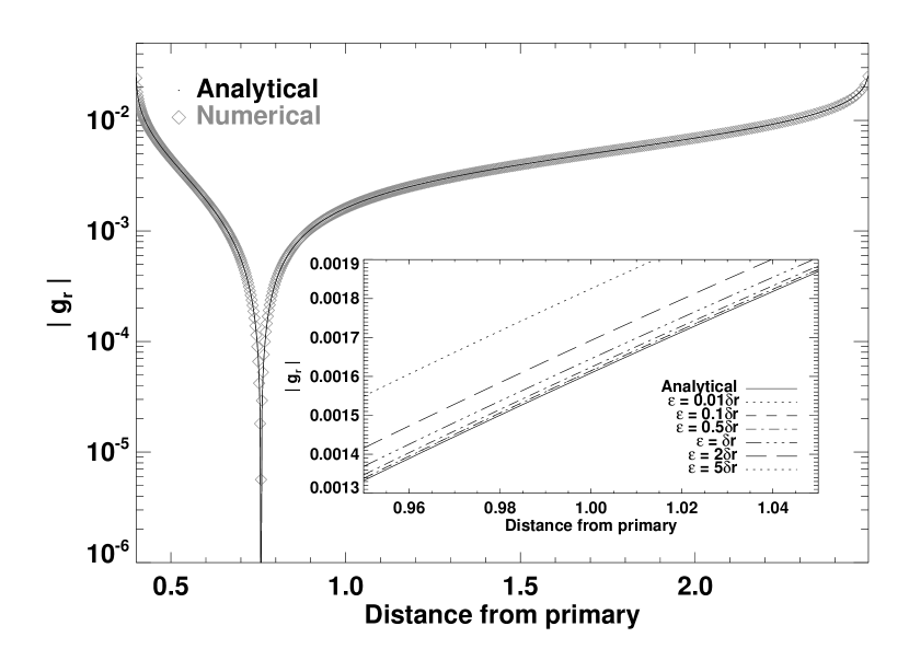
Figure 1: Radial self-gravitating acceleration $g_{r}(r)$, in absolute value, for a uniform surface density field. The analytical expression of $g_{r}$ [see Eq. (1)] is compared with the result of a self-gravitating calculation with a small softening length (see text). We point out that $g_{r}(r)$ is positive at the inner edge, then it becomes negative (here from $r\gtrsim 0.75$). The close-up reveals the influence of the softening length on the agreement between the numerical calculation and the analytical expectation (see text).

2.2.2 Numerical issues

The implementation of the disk self-gravity addresses two issues. The first one concerns the convergence properties of our results. We performed preliminary runs to check the torque convergence, without and with self-gravity. The computational domain is covered with $N_{r}$ zones radially between $r_{\rm min}=0.4r_{p}$ and $r_{\rm max}=2.5r_{p}$, and $N_{\varphi}$ zones azimuthally between $\varphi=0$ and $\varphi=2\pi$. For a comparative purpose, a logarithmic radial spacing is also used for the calculations without self-gravity. We adopted disk parameters and a planet mass that are representative of our study, namely a $Q=8$ Toomre parameter at the planet location, and a $M_{p}=5\times 10^{-6}M_{*}$ planet mass. A complete description of our model parameters is deferred to section 2.3. We evaluate the torque obtained without self-gravity ($\Gamma_{\rm nog}$) and with self-gravity ($\Gamma_{\rm fsg}$) for several pairs ($N_{r},N_{\varphi}$). The relative difference of these torques is displayed in Fig. 2a. We see in particular that the torque convergence is already achieved for $N_{r}=512$ and $N_{\varphi}=1536$, values that we adopted for all the calculations of this paper.

Furthermore, since the softening length $\varepsilon_{\rm sg}$ varies from one ring to another, the FFT algorithm does not ensure an exact action-reaction reciprocity. Thus, the disk self-gravity may worsen the conservation of the total angular momentum (that of the system {gas+planet}). To investigate this issue, we performed calculations with a planet migrating in a disk without and with self-gravity. For these calculations only, the disk is inviscid, and reflecting boundaries are adopted. As for the above convergence study, we adopted a $M_{p}=5\times 10^{-6}M_{*}$ planet mass, and a $Q=8$ Toomre parameter at the planet location. The value of $\varepsilon_{\rm sg}(r_{p})$ is the one used in our calculations hereafter (see section 2.3). We display in Fig. 2b the torques on the planet ($\Gamma_{\rm planet}$) and on the whole system ($\Gamma_{\rm planet+gas}$), for both calculations. If the code were perfectly conservative, the ratio $\Gamma_{\rm planet+gas}/\Gamma_{\rm planet}$ would cancel out, to within the machine precision. This ratio is typically $\sim 0.5$ % without self-gravity, and $\sim 3$ % with self-gravity. Although, as expected, the conservation of the total angular momentum is worse with self-gravity, it remains highly satisfactory.

Figure 2: Left: Relative difference of the torques obtained without self-gravity ($\Gamma_{\rm nog}$), and with self-gravity ($\Gamma_{\rm fsg}$), for different grid resolutions (see text). Right: Torque exerted on a $M_{p}=5\times 10^{-6}$ planet mass, and on the system {gas+planet}. Torques are depicted for a calculation without self-gravity (long-dashed and dash-dotted curves), and with self-gravity (solid and dotted curves).

2.3 Model parameters

In the runs presented hereafter, the disk surface density $\Sigma$ is initially axisymmetric with a power-law profile, $\Sigma(r)=\Sigma_{p}(r/r_{p})^{-\sigma}$, where $\Sigma_{p}$ is the surface density at the planet’s orbital radius. The reference value of $\sigma$ is $3/2$. We therefore expect the corotation torque, which scales with the gradient of (the inverse of) the disk vortensity, to cancel out for a non self-gravitating disk (Ward, 1991; Masset, 2001).

The vertically integrated pressure $p$ and $\Sigma$ are connected by an isothermal equation of state, $p=\Sigma{c_{s}}^{2}$, where $c_{s}$ is the local isothermal sound speed. The disk aspect ratio is $h(r)=H(r)/r=c_{s}(r)/r\Omega_{K}(r)$, where $H(r)$ is the disk scale height at radius $r$, and $\Omega_{K}$ denotes the Keplerian angular velocity. We take $h$ uniform, ranging from $h=0.03$ to $h=0.05$, depending on the calculations. We use a uniform kinematic viscosity $\nu$, which is $10^{-5}$ in our unit system.

The gravitational forces exerted on the disk include:

• The gravity of the central star.

• The gravity of an embedded planet, whose potential is a Plummer one with softening parameter $\varepsilon=0.3H(r_{p})$.

• The disk self-gravity, whenever it is mentioned. The self-gravity softening length $\varepsilon_{\rm sg}$ is chosen to scale with $r$, and to be equal to $\varepsilon$ at the planet’s orbital radius, which yields $\varepsilon_{\rm sg}(r)=\varepsilon\,r/r_{p}$. Since $h$ is taken uniform, $H(r)$ scales with $r$, and $\varepsilon_{\rm sg}(r)=0.3H(r)$. We comment that $\varepsilon_{\rm sg}(r_{p})$ is very close to the recent prescription of Huré & Pierens (2006) for the softening length of a flat, axisymmetric self-gravitating disk. From now on, whenever we mention the softening length, we will refer to $\varepsilon$.

The disk’s initial rotation profile $\Omega(r)$ is slightly sub-Keplerian, the pressure gradient being accounted for in the centrifugal balance. When the disk self-gravity is taken into account, it reads

$$\Omega(r)=\left(\Omega_{K}^{2}(r)\left[1-(1+\sigma)h^{2}\right]-\frac{g_{r}(r)}{r}\right)^{1/2}.$$ (2)

We comment that $g_{r}(r)$ is not necessarily a negative quantity. When it is so, the disk rotates slightly faster with self-gravity than without. In a two-dimensional truncated disk, $g_{r}$ is positive at the inner edge and becomes negative at a distance from the inner edge that depends on $\sigma$. We checked that, whatever the values of $\sigma$ used in this paper, $g_{r}$ is always negative in a radial range around the planet’s orbital radius that is large enough to embrace all Lindblad resonances (except the inner Lindblad resonance of $m=1$ for $\sigma=0$, as can be inferred from Fig. 1).

As stated in section 2.2.2, our calculations are performed on a grid with a logarithmic radial spacing, even when the disk self-gravity is not taken into account. The resolution is therefore the same in all our calculations. The computational domain is covered with $N_{r}=512$ zones radially between $r_{\rm min}=0.4r_{p}$ and $r_{\rm max}=2.5r_{p}$, and $N_{\varphi}=1536$ zones azimuthally between $\varphi=0$ and $\varphi=2\pi$.

3 Dependence of the differential Lindblad torque on the disk surface density

Our study is restricted to the linear regime, which enables us to compare the results of our calculations with analytical predictions. For this purpose, we consider a $q=5\times 10^{-6}$ planet to primary mass ratio. According to Masset et al. (2006a), for a two-dimensional calculation, the flow in the planet vicinity remains linear as long as

$$r_{\rm B}\ll\varepsilon,$$ (3)

where $r_{\rm B}=GM_{p}/c_{s}^{2}(r_{p})$ is the planet’s Bondi radius and $\varepsilon$ is the softening length. Eq. (3) translates into $q\ll q_{\rm lin}$, with $q_{\rm lin}=0.3h^{3}$ in our units. For a $h=5$ % disk aspect ratio, $q_{\rm lin}\approx 4\times 10^{-5}$ so that our planet mass is well inside the linear regime. For a $h=3$ % disk aspect ratio, $q_{\rm lin}\approx 8\times 10^{-6}$ and our planet mass approximately fulfills the linearity condition. Note that the linearity criterion given by Eq. (3) ensures that the torque $\Gamma$ exerted by the disk on the planet scales with $q^{2}$. We focus in this section on the scaling of $\Gamma$ with $\Sigma_{p}$, scaling that is expected, for a non self-gravitating disk, as long as the planet does not open a gap. The gap clearance criterion, recently revisited by Crida et al. (2006), reads in our unit system

$$\frac{3}{4}\,h\left(\frac{q}{3}\right)^{-1/3}+50\frac{\nu}{q}\leq 1.$$ (4)

The L.H.S. of Eq. (4) is $\sim 100$, hence we expect to check $\Gamma\propto\Sigma_{p}$ in our calculations without self-gravity.

The runs presented hereafter lasted for $20$ orbits, which was long enough to get stationary values of the torque. For the calculations without self-gravity, the torque evaluation takes all the disk into account, it does not exclude the content of the planet’s Hill sphere. We checked that excluding it or not makes no difference in the torque measurement. This is consistent with the fact that, for the planet mass considered here, we do not find any material trapped in libration around the planet, be it inside a circumplanetary disk (a fraction of the planet’s Hill radius) or inside a Bondi sphere.

3.1 Case of a non self-gravitating disk

Table 1: Planet’s angular velocity $\Omega_{p}(r_{p})$ and disk’s rotation profile $\Omega(r)$ for a non self-gravitating disk

	fixed case	free case
$\Omega_{p}(r_{p})$	$\Omega_{K}(r_{p})$	$\left(\Omega_{K}^{2}(r_{p})-\frac{g_{r}(r_{p})}{r_{p}}\right)^{1/2}$
$\Omega(r)$	$\Omega_{K}(r)\left[1-(1+\sigma)h^{2}\right]^{1/2}$	$\Omega_{K}(r)\left[1-(1+\sigma)h^{2}\right]^{1/2}$

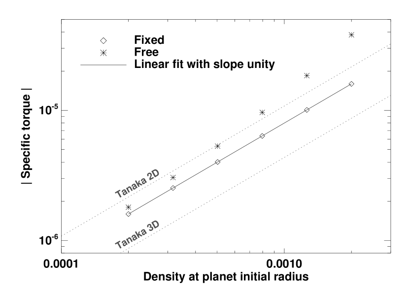
Figure 3: Specific torque $\gamma$ exerted on a $M_{p}=5\times 10^{-6}M_{*}$ planet mass by a non self-gravitating disk, with a $h=5$ % aspect ratio. Diamonds refer to the fixed case (the planet is held on a fixed circular orbit, with a strictly Keplerian angular velocity) while asterisks refer to the free case (the planet freely evolves in the disk, the planet’s angular velocity is greater than Keplerian). The solid line corresponds to a proportional fit of the fixed case data, and shows the excellent agreement between our results of calculations and the expectation $\gamma\propto\Sigma_{p}$ in the fixed case. The two dotted lines depict the two- and three-dimensional analytical estimates of Tanaka et al. (2002).

We first tackle the case of a non self-gravitating disk. We measure the specific torque $\gamma=\Gamma/q$ on the planet for six different values of $\Sigma_{p}$, ranging from $\Sigma_{p}=2\times 10^{-4}$ to $\Sigma_{p}=2\times 10^{-3}$. This corresponds to varying the initial disk surface density at the planet’s orbital radius from one to ten times the surface density of the minimum mass solar nebula (MMSN). Two situations are considered (see also Table 1):

• On the one hand, the planet does not feel the disk gravity: it is held on a fixed circular orbit, with a strictly Keplerian orbital velocity. In this case, referred to as the fixed case, both the planet and the disk feel the star gravity but do not feel the disk gravity. The disk non-Keplerianity is exclusively accounted for by the radial pressure gradient. This is the configuration that has been contemplated in analytical torque estimates (see e.g. Tanaka et al., 2002).

• On the other hand, the planet feels the disk gravity. In other words, we let the planet evolve freely in the disk, so its angular velocity, which reads

  $$\Omega_{p}(r_{p})=[\Omega_{K}^{2}(r_{p})-g_{r}(r_{p})/r_{p}]^{1/2},$$ (5)

  is slightly greater than Keplerian. In this case, which we call the free case, the planet feels the gravity of the star and of the disk while, as previously stated, the disk does not feel its own gravity. Contrary to the fixed case, the free case is not a self-consistent configuration since the planet and the disk do not orbit under the same gravitational potential. Nevertheless, this situation is of interest as it corresponds to the standard scheme of all simulations dealing with the planet-disk tidal interaction.

We show in Fig. 3 the specific torques (in absolute value) obtained with the fixed and free cases, for a $h=0.05$ disk aspect ratio. In the fixed situation, there is an excellent agreement with the expectation $\gamma\propto\Sigma_{p}$, and, not surprisingly, the torques are bounded by the two- and three-dimensional analytical estimates of Tanaka et al. (2002). Nonetheless, the free case reveals two unexpected results. For a given surface density, the absolute value of the torque is larger than expected from the fixed case. Moreover, it increases faster than linearly with the disk surface density.

Figure 4: Location of two Lindblad resonances in the fixed case (left panel) and in the free case (right panel): the ILR of $m=6$ ($\Omega_{\rm ILR}=6/5\,\Omega_{p}$), and the OLR of $m=5$ ($\Omega_{\rm OLR}=5/6\,\Omega_{p}$). The disk’s rotation profile $\Omega(r)$ is depicted without self-gravity (solid curve) and with self-gravity (dashed curve, right panel). In the latter case, $g_{r}(r)$ is given by a calculation with $\Sigma_{p}=5\times 10^{-2}$, a value exaggerated to improve legibility. Note also that the pressure buffer has been discarded in both profiles, for the sake of simplicity. The vertical arrow at $r=1$ indicates the planet location, it reaches the upper curve in the free case (right panel) since the planet feels the disk gravity. The ILR and OLR are located, respectively, at $r_{\rm ILR}=\Omega^{-1}(\Omega_{\rm ILR})$ and $r_{\rm OLR}=\Omega^{-1}(\Omega_{\rm OLR})$. The nominal position of the resonances (that of the fixed case) is indicated by light gray dash-dotted lines on the right panel to appreciate their shift, highlighted by a horizontal arrow.

The two latter results can be explained with the relative positions of the Lindblad Resonances (hereafter LR) in the fixed and free cases. We display in Fig. 4a the locations $r_{\rm ILR}$ ($r_{\rm OLR}$) of an Inner (Outer) LR, when the planet is on a fixed orbit. They are given by $r_{\rm ILR}=\Omega^{-1}(\Omega_{\rm ILR})$ and $r_{\rm OLR}=\Omega^{-1}(\Omega_{\rm OLR})$, with $\Omega(r)$ the disk’s rotation profile (solid curve), and $\Omega_{\rm ILR}$ ($\Omega_{\rm OLR}$) the frequency of the ILR (OLR), simply deduced from the planet frequency $\Omega_{p}$.

When the planet is on a free orbit (Fig. 4b), its frequency is slightly larger than in the fixed case. Thus, the frequencies of the LR are also larger in the free case, which induces a spurious inward shift of all the resonances. The OLR get closer to the orbit, which increases the (negative) outer Lindblad torque. The ILR are shifted away from the orbit, which reduces the (positive) inner Lindblad torque. Thus, the (negative) differential Lindblad torque is artificially larger in the free case.

The inward shift of the LR, which we denote by $\delta R$, has been evaluated analytically by PH05. A simple estimate can be obtained as follows. We denote by $R_{*}$ the nominal position of the resonances without disk gravity. We assume that the disk’s rotation profile is strictly Keplerian. The shift $\delta R$ being induced by the increase of the planet frequency, we have $\delta R/R_{*}=-2\delta\Omega_{p}(r_{p})/3\Omega_{K}(r_{p})$, where $\delta\Omega_{p}(r_{p})$ is the difference of the planet frequencies between the free and fixed cases. Using Eq. (5) and a first-order expansion, we are left with

$$\frac{\delta R}{R_{*}}=\frac{g_{r}(r_{p})}{3r_{p}\Omega_{K}^{2}(r_{p})}.$$ (6)

A more accurate expression for $\delta R/R_{*}$ is given by PH05 [see their equation (7c)]. Eq. (6) shows that the shift of the LR scales with $g_{r}(r_{p})$, hence with $\Sigma_{p}$. This explains why the torque in the free case increases faster than linearly with the disk surface density. The relative shift of the resonances $\delta R/R_{*}$ typically amounts from $-3\times 10^{-4}$ to $-3\times 10^{-3}$ for our range value of surface densities, corresponding however to a torque relative discrepancy between $\sim 12$ % and $\sim 120$ % (see Fig. 3).

Figure 5: Relative difference of the torques between the free and fixed situations, as a function of $Qh$ [see text and Eq. (7)].

We are primarily interested in a quantitative comparison of the torques in the fixed and free cases. Nonetheless, since the shift of the LR scales with $g_{r}(r_{p})$, it depends on the mass distribution of the whole disk. Thus, the torque discrepancy between the fixed and free cases also depends on $g_{r}(r_{p})$, hence on $\Sigma_{p}$, $\sigma$, $r_{\rm min}$ and $r_{\rm max}$. In particular, we point out that if the planet is close enough to the disk’s inner edge, then $g_{r}(r_{p})$ can be positive (see Fig. 1, for $\sigma=0$). This shifts all the LR outward (instead of inward) and reduces the torque. We have checked this prediction with an appropriate calculation (not presented here).

In our study, only $\Sigma_{p}$ is a free parameter. The index of the unperturbed surface density profile, $\sigma$, is fixed indeed to $3/2$, as explained in section 2.3. Our values of $r_{\rm min}$ and $r_{\rm max}$ are those customarily used in numerical simulations of planet-disk interactions (see e.g. de Val-Borro et al., 2006). Thus, a useful quantitative comparison of the torques between the free and fixed cases can be provided just by varying $\Sigma_{p}$. In particular, one may think the torque discrepancy to be significant only for high values of $\Sigma_{p}$. Nevertheless, such a discrepancy depends both on the surface density $\Sigma_{p}$ and on the disk aspect ratio $h$. As explained in Appendix B, we expect the relative difference of the torques between the free and fixed situations to scale with $(Qh)^{-1}$, where $Q$ is the Toomre parameter at the planet’s orbital radius,

$$Q=\left[\frac{c_{s}\kappa}{\pi G\Sigma}\right]_{r_{p}}\equiv h/m_{D},$$ (7)

with $\kappa$ the horizontal epicyclic frequency, defined as $\kappa=\left[2\Omega r^{-1}\,d(r^{2}\Omega)/dr\right]^{1/2}$, and $m_{D}=\pi r_{p}^{2}\Sigma_{p}/M_{*}$. Eq. (7) can be recast as $Q=h/\pi\Sigma_{p}$ in our units.

To study the impact of $h$ on previous results, we performed another set of calculations with $h=0.03$. Fig. 5 confirms that the relative difference of the torques scales with the inverse of $Qh$. It yields an estimate of the error done on the torque evaluation when involving the strongly biased free situation rather than the self-consistent fixed situation. For instance, for a $h=3$ % disk aspect ratio, the free situation can overestimate the torque by as much as a factor two in a disk that has only $\sim 3$ times the disk surface density of the MMSN. Moreover, the torque relative difference is less than $20$ % as long as $Qh\gtrsim 2.5$, hence as long as the Toomre parameter at the planet location is approximately greater than $50$ if $h=0.05$, or $80$ if $h=0.03$. Remember that these estimates depend on the precise value of $g_{r}(r_{p})$, hence on the mass distribution of the whole disk. They are provided with fixed, but customarily used values of $\sigma$, $r_{\rm min}$ and $r_{\rm max}$.

To avoid the above torque discrepancy, one must ensure that the planet and the disk feel the same gravitational potential. The workaround depends on whether the disk is self-gravitating or not, and whether the planet freely migrates in the disk or not:

1. The disk is not self-gravitating. The planet’s angular velocity should therefore be strictly Keplerian:

   1. The planet evolves freely in the disk. Thus, its angular velocity, given by Eq. (5), is slightly greater than Keplerian. A workaround could be to subtract the axisymmetric component of the disk surface density to the surface density before calculating the force exerted on the planet by the disk. This would cancel out $g_{r}(r_{p})$, and the planet’s angular velocity would remain strictly Keplerian.

   2. The planet is held on a fixed circular orbit, with necessarily a Keplerian angular velocity. This is a self-consistent situation.

2. The disk is self-gravitating. The planet’s angular velocity should therefore be given by Eq. (5):

   1. The planet evolves freely in the disk. This is a self-consistent situation.

   2. The planet is held on a fixed circular orbit. This situation is self-consistent only if the planet’s fixed angular velocity is given by Eq. (5).

From now on, whenever calculations without disk gravity are mentioned, they refer to the fixed situation. We mention them as nog calculations.

3.2 Case of a self-gravitating disk

Table 2: Planet’s angular velocity $\Omega_{p}(r_{p})$ and disk’s rotation profile $\Omega(r)$, without and with disk gravity

	Without disk gravity	With disk gravity
$\Omega_{p}(r_{p})$	$\Omega_{K}(r_{p})$	$\left(\Omega_{K}^{2}(r_{p})-\frac{g_{r}(r_{p})}{r_{p}}\right)^{1/2}$
$\Omega(r)$	$\Omega_{K}(r)\left[1-(1+\sigma)h^{2}\right]^{1/2}$	$\left(\Omega_{K}^{2}(r)\left[1-(1+\sigma)h^{2}\right]-\frac{g_{r}(r)}{r}\right)^{1/2}$

Figure 6: Specific torque on a $M_{p}=5\times 10^{-6}M_{*}$ planet mass, obtained with axisymmetric and fully self-gravitating calculations, with a $h=5$ % disk aspect ratio. Torques achieved without disk gravity (see section 3.1) are also displayed, for comparison.

We study how the results of section 3.1 differ when the disk gravity is felt both by the planet and the disk. The planet is still held on a fixed circular orbit at $r=r_{p}$, its angular velocity is given by Eq. (5). As in the situation without disk gravity, the planet’s initial velocity is that of a fluid element that would not be subject to the radial pressure gradient (see Table 2).

Taking the disk self-gravity into account induces two shifts of Lindblad resonances (PH05): (i) a shift arising from the axisymmetric component of the disk self-gravity, and (ii) a shift stemming from the non-axisymmetric component of the disk self-gravity. We therefore performed two series of calculations:

1. Calculations that involve only the axisymmetric part of the disk self-gravity. They are mentioned as axisymmetric self-gravitating calculations (asg calculations). Their computational cost is the same as that of a calculation without disk gravity since only one-dimensional FFTs are performed. The results of these calculations are presented in section 3.2.1.

2. Fully self-gravitating calculations (fsg calculations), which are more computationally expensive as they involve two-dimensional FFTs. Their results are presented in section 3.2.2.

3.2.1 Axisymmetric self-gravitating calculations

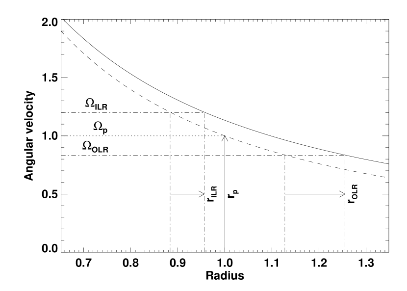
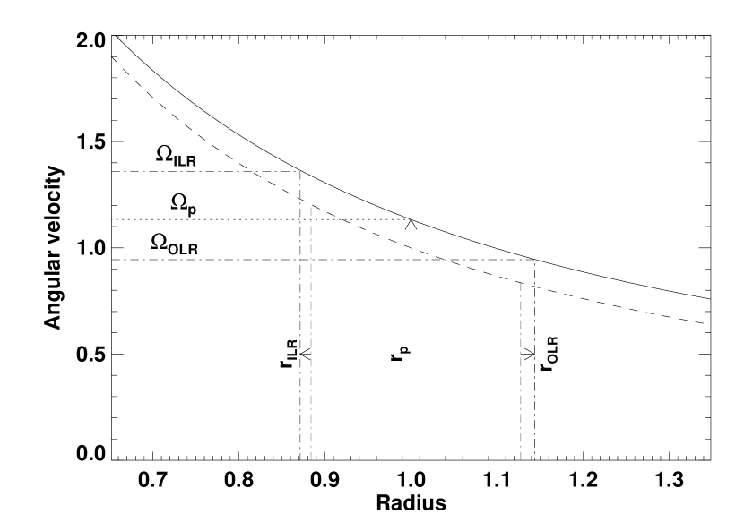
Figure 7: Same as Fig. 4, except that we examine the shift of the LR when the disk is self-gravitating (its rotation profile is now the solid, upper curve). In the left panel, the planet does not feel the disk gravity: the frequency of the planet, and therefore that of the LR, is the same as in Fig. 4a. In the right panel, both the planet and the disk feel the disk gravity: the frequencies of the planet and of the LR are those of Fig. 4b.

We display in Fig. 6 the torques obtained with the nog, asg and fsg calculations, when varying $\Sigma_{p}$. We will comment the results of the fsg calculations in section 3.2.2. The torques obtained in the asg situation, which we denote by $\gamma_{\rm asg}$, are hardly distinguishable from the torques without disk gravity, mentioned as $\gamma_{\rm nog}$. A straightforward consequence is that $\gamma_{\rm asg}$ scales with $\Sigma_{p}$ with a good level of accuracy. We point out however that the torque difference $|\gamma_{\rm asg}|-|\gamma_{\rm nog}|$ is slightly negative and decreases with $\Sigma_{p}$ (not displayed here). The relative difference $|\,|\gamma_{\rm asg}|-|\gamma_{\rm nog}|\,|/|\gamma_{\rm nog}|$ varies from $\sim 0.2$ % for $\Sigma_{p}=2\times 10^{-4}$, to $\sim 2$ % for $\Sigma_{p}=2\times 10^{-3}$.

The interpretation of these results is as follows. In the asg situation, the positions of the LR related to the Fourier component with wavenumber $m$ are the roots of equation (see PH05 and references therein)

$$D_{\rm asg}(r)=\kappa^{2}(r)-m^{2}[\Omega(r)-\Omega_{p}]^{2}+m^{2}c_{s}^{2}(r)/r^{2}=0,$$ (8)

where, contrary to the nog situation, $\Omega(r)$ and $\Omega_{p}$ depend on $g_{r}$ (see Table 2). As in section 3.1, the increase of the planet frequency implies an inward shift of the LR, which increases the differential Lindblad torque (see Fig. 4b). Furthermore, as pointed out in Fig. 7a, the increase of the disk frequency causes an outward shift of all LR, which reduces the differential Lindblad torque. Accounting for the axisymmetric component of the disk gravity therefore leads to two shifts of the resonances, acting in opposite ways. Fig. 7b shows that both shifts do not compensate exactly: the LR are slightly moved away from corotation with respect to their nominal position without disk gravity. This is in qualitative agreement with PH05, who found a resulting shift which is negative for inward resonances, and positive for outward resonances (see their $\delta R_{1}+\delta R_{3}$ expression). The sign of the shift results from the fact that the disk’s rotation profile decreases more slowly with self-gravity than without, and explains why $|\gamma_{\rm asg}|-|\gamma_{\rm nog}|$ is negative. The absolute value of this shift increases with $\Sigma_{p}$, which entails that $||\gamma_{\rm asg}|-|\gamma_{\rm nog}||$ increases with $\Sigma_{p}$.

3.2.2 Fully self-gravitating calculations

Figure 8: Relative difference of the torques obtained with the fully self-gravitating calculations ($\gamma_{\rm fsg}$) and the calculations without disk gravity ($\gamma_{\rm nog}$), as a function of the Toomre parameter $Q$ at the planet location.

We now come to the results of the fsg calculations depicted in Fig. 6. The torques obtained with the fsg calculations, denoted by $\gamma_{\rm fsg}$, are larger than $\gamma_{\rm asg}$ and $\gamma_{\rm nog}$. Moreover, $|\gamma_{\rm fsg}|$ grows faster than linearly with the disk surface density, a result already mentioned by Tanigawa & Lin (2005).

These results can be understood again in terms of shifts of the LR. Besides the shift due to the slight increase of the planet and of the disk frequency, the fsg situation triggers another shift stemming from the additional non-axisymmetric term $-2\pi G\Sigma m/r$ in the dispersion relation of density waves (in the WKB approximation, see PH05). The positions of the LR associated with wavenumber $m$ are this time the roots of equation

$$D_{\rm fsg}(r)=D_{\rm asg}(r)-2\pi G\Sigma(r)m/r=0,$$ (9)

where $D_{\rm asg}$ is given by Eq. (8). PH05 showed that:

• This non-axisymmetric contribution moves inner and outer LR toward the orbit, with respect to their location in the asg situation. This explains why $|\gamma_{\rm fsg}|>|\gamma_{\rm asg}|$, and implies that the torque variations at inner and outer resonances have opposite signs.

• The shift induced by the non-axisymmetric part of the disk self-gravity dominates that of its axisymmetric component. Therefore, it approximately accounts for the total shift due to the disk gravity, and explains why $|\gamma_{\rm fsg}|>|\gamma_{\rm nog}|\approx|\gamma_{\rm asg}|$.

• This shift increases with $\Sigma_{p}$, so that $|\gamma_{\rm fsg}|$ increases faster than linearly with $\Sigma_{p}$.

Our results of calculations are in qualitative agreement with the analytical work of PH05. Before coming to a quantitative comparison in section 3.3.2, we focus on the relative difference of the torques between the fsg and nog situations. From previous results, we assume that the only shift of the LR is due to the non-axisymmetric part of the disk gravity. Interestingly, this shift does not feature $g_{r}$, so it does not depend on the mass distribution of the whole disk. It only depends on the surface density at the planet location. Since the torque variations at inner and outer resonances are of opposite sign, we expect the relative difference of the torques to scale with $Q^{-1}$, for high to moderate values of $Q$. This is shown in Appendix C. It differs from the $(Qh)^{-1}$ scaling obtained in Fig. 5, where the torque variations at inner and outer resonances were of identical sign.

In Fig. 8, we plot this relative difference as a function of $Q$ for previous results and for another series of runs performed with a $h=0.03$ disk aspect ratio. The departure from the expected scaling occurs for $Q\lesssim 6$. The behavior at low $Q$ will be tackled in section 3.3.2. Fig. 8 yields a useful estimate of the torque increase due to the disk gravity, or, differently stated, of the torque underestimate if one discards the disk gravity. As such estimate only depends on the Toomre parameter at the planet location, whatever the global mass distribution of the disk. The torques’ relative difference is typically one order of magnitude smaller than in the situation of a planet freely migrating in a non self-gravitating disk (Fig. 5). It amounts typically to $10$ % for $Q\approx 10$. For $Q\gtrsim 50$, accounting for the disk gravity or not has no significant impact on the torque measurement.

Our results confirm that the disk gravity accelerates type I migration. This might sound contradictory with the results of Nelson & Benz (2003a, b), who found that the disk self-gravity slows down migration for a planet that does not open a gap. The authors compared however the results of their self-gravitating calculations (where both the planet and the disk feel the disk gravity) to those obtained with the misleading situation of a planet freely migrating in a disk without self-gravity. As shown by Fig. 9, or as can be inferred from Figs. 3 and 6, comparing both situations would lead us to the same conclusion. There is therefore no contradiction between their findings and ours. From now on, we do not distinguish the gravity and self-gravity designations, since the planet and the disk orbit within the same potential in our calculations. Whenever calculations with disk gravity are mentioned, they refer to the fsg situation.

Figure 9: Specific torque variation with time, with and without disk gravity. In each case, two situations are depicted: the fixed case (the planet is on a fixed orbit with the appropriate angular velocity, see Table 2) and the free case (the planet is free to migrate in the disk). Except the self-gravitating calculation with a free planet, the calculations are those of Figs. 3 and 6 for $\Sigma_{p}=2\times 10^{-3}$. When the planet in on a free orbit without self-gravity, the torque oscillates with a large amplitude. This is due to the slight increase of the planet frequency: $\Omega_{p}(r_{p})$, which is initially strictly Keplerian, is given by Eq. (5) during its time evolution.

3.3 Comparison with analytical results

3.3.1 An analytical estimate

We propose in this section a simple analytical estimate of the relative difference of the torques between the fsg and nog situations. This estimate concerns high to moderate values of the Toomre parameter at the planet location. We assume that the only shift of the LR in the fsg situation arises from its non-axisymmetric contribution. This comes to approximating the nog and asg situations, which is a reasonable assumption from Fig. 6. Furthermore, since this shift has same order of magnitude at inner and outer LR (PH05), we focus on the one-sided Lindblad torque and use a local shearing sheet approximation. We set up local Cartesian coordinates ($x$, $y$) with origin at the planet position, the $x$ and $y$-axis pointing toward the radial and azimuthal directions. Our $x$-coordinate is taken normalized as

$$x=\frac{r-r_{p}}{H(r_{p})}=\frac{r-r_{p}}{hr_{p}}.$$ (10)

As is usually done in the shearing sheet framework, we discard the radial dependence of the disk surface density and scale height (Narayan et al., 1987). In a non-gravitating disk, the LR associated with wavenumber $m$ are therefore located at

$$x_{\rm nog}=\frac{2}{3}\epsilon\frac{\sqrt{1+\xi^{2}}}{\xi},$$ (11)

where $\xi=mh$, $\epsilon=+1$ for outer resonances, $\epsilon=-1$ for inner resonances. In the fsg situation, LR are located at $x_{\rm nog}+\delta x_{\rm fsg}$, where the shift $\delta x_{\rm fsg}$ is evaluated by $D_{\rm fsg}(x_{\rm nog}+\delta x_{\rm fsg})=0$. Using Eqs. (8), (9) and (11), a first-order expansion yields

$$\delta x_{\rm fsg}=-\frac{2}{3\epsilon Q}\frac{1}{\sqrt{1+\xi^{2}}}.$$ (12)

We comment that the equation (7b) of PH05 reduces to our Eq. (12) for a surface density profile decreasing as $r^{-3/2}$.

In the linear regime, the one-sided Lindblad torque $\Gamma$ amounts to a summation over $m$ of the Fourier components $\Gamma_{m}$. In the shearing sheet approximation, since all quantities depend on $m$ through $\xi$, the summation over $m$ is approximated as an integral over $\xi$,

$$\Gamma=\frac{1}{h}\int_{0}^{\infty}T(x=x_{L},\xi)~{}d\xi,$$ (13)

where $x_{L}$ denotes the positions of the LR, $T$ is the $m^{\rm th}$ Fourier component of the one-sided Lindblad torque, given by (see e.g. Ward, 1997)

$$T(x,\xi)=K\frac{\xi^{2}\Psi^{2}(x,\xi)}{\sqrt{1+\xi^{2}}(1+4\xi^{2})},$$ (14)

with $K$ a constant. We assume that Eq. (14) can be used whatever the disk is self-gravitating or not (Goldreich & Tremaine, 1979). The forcing function $\Psi$ in Eq. (14) is approximated in a standard way as a function of the Bessel $K_{0}$ and $K_{1}$ functions,

$$\Psi(x,\xi)=K_{1}(|x|\xi)+2\sqrt{1+\xi^{2}}K_{0}(|x|\xi).$$ (15)

We furthermore approximate $\Psi(x,\xi)$ as $(|x|\xi)^{-1}$, to within a numerical factor of the order of unity (Abramowitz & Stegun, 1972). This approximation is valid when $\xi\lesssim 1$, hence for low $m$-values.

With a first-order expansion in $Q^{-1}$, the difference of the one-sided Lindblad torques between the fsg and nog situations reads

$$\Gamma_{\rm fsg}-\Gamma_{\rm nog}\approx\frac{1}{h}\int_{0}^{\infty}\left(\frac{\partial T}{\partial x}\right)_{x=x_{\rm nog},\xi}\delta x_{\rm fsg}\,d\xi.$$ (16)

Combining Eqs. (11) to (16), we are left with

$$\left|\frac{\Gamma_{\rm fsg}-\Gamma_{\rm nog}}{\Gamma_{\rm nog}}\right|=\frac{2I}{3Q},$$ (17)

where

$$\left.I\right. ~{}=~{} 3\times\,\frac{\displaystyle\int_{0}^{\infty}\frac{\xi^{3}}{(1+\xi^{2})^{5/2}(1+4\xi^{2})}d\xi}{\displaystyle\int_{0}^{\infty}\frac{\xi^{2}}{(1+\xi^{2})^{3/2}(1+4\xi^{2})}d\xi}$$ (18)

$$~{}=~{} \frac{2\sqrt{3}-\log{(7+4\sqrt{3})}}{\sqrt{3}-\pi/3}\;\approx\;1.21.$$

Not surprisingly, the relative difference of the one-sided Lindblad torques scales with the inverse of $Q$. This is the same scaling as for the relative difference of the differential Lindblad torques, assuming high to moderate values of $Q$ (see Appendix C and Fig. 8). Note that, unlike the analysis of PH05, the present analysis, which is restricted to the shearing-sheet framework, enables one to exhibit the $Q^{-1}$ scaling given by Eq. (17).

3.3.2 Results

We come to a quantitative comparison of our results of calculations with our analytical estimate, given by Eq. (17), and the analytical results of PH05, who estimated the dependence of the differential Lindblad torque on the disk mass, for a fully self-gravitating disk (see their figure 4b). Another series of fsg calculations was performed with disk parameters similar to those of PH05, namely a $h=5$ % disk aspect ratio, a planet mass corresponding to the linear regime (its value is precised hereafter). We vary the disk surface density at the planet’s orbital radius from $\Sigma_{p}=4\times 10^{-4}$ to $\Sigma_{p}=10^{-2}$. This corresponds to varying $Q$ from $40$ to $1.6$. The runs lasted for $10$ planet’s orbital periods, which was long enough to get stationary torques for the largest values of $Q$, but short enough to avoid a significant growth of non-axisymmetric perturbations for the lowest values of $Q$, probably due to SWING amplification (Toomre, 1964).

As we aim at comparing the results of two-dimensional calculations with analytical expectations (for which there is no softening parameter), we investigated how much our results of calculations depend on the softening length. For this purpose, the calculations were performed with three values of $\varepsilon$: $0.1H(r_{p})$, $0.3H(r_{p})$ and $0.6H(r_{p})$. The planet mass is $M_{p}=4.4\times 10^{-6}M_{*}$ for $\varepsilon=0.3H(r_{p})$ and $\varepsilon=0.6H(r_{p})$, whereas $M_{p}=10^{-6}M_{*}$ for $\varepsilon=0.1H(r_{p})$. This choice ensures that the Bondi radius to softening length ratio does not exceed $\sim 10$ % for each value of $\varepsilon$.

Each calculation was performed with and without disk gravity, so as to compute the relative difference of the torques between both situations. The reason why we compute this relative difference is that it does not depend on the details of the torque normalization, be it for the numerical or the analytical results. Nonetheless, PH05 only calculated the normalized torque in the fsg situation as a function of the disk mass. We then evaluated their normalized torque without disk gravity by extrapolating their torque with disk gravity in the limit where the disk mass tends to zero.

Figure 10: Relative difference of the torques between with the fsg situation ($\gamma_{\rm fsg}$) and the nog situation ($\gamma_{\rm nog}$) as a function of the disk surface density $\Sigma_{p}$. We compare the results of our calculations (each symbol refers to a different value of the softening length $\varepsilon$) with the analytical results of PH05 (dashed curve), and our analytical estimate (dash-dotted curve, see text and Eq. (17)). The vertical dotted lines display different values of the Toomre parameter at the planet location.

Fig. 10 displays the relative difference of the torques between the fsg situation ($\gamma_{\rm fsg}$) and the nog situation ($\gamma_{\rm nog}$), obtained with our calculations, the analytical expectation of PH05 and our analytical estimate. This relative difference grows faster than linearly with $\Sigma_{p}$, although a linear approximation is valid at low surface density, as already stated in section 3.2.2. Our linear estimate is in agreement with the results of calculations with $\varepsilon=0.6H(r_{p})$ up to $Q\sim 3$, where it leads to a torque enhancement that is typically half the one estimated by PH05. Furthermore, our results of calculations depend much on $\varepsilon$, more especially at high $\Sigma_{p}$. For a given value of $\Sigma_{p}$, the relative difference of the torques decreases as $\varepsilon$ increases. Differently stated, increasing the softening length reduces $\gamma_{\rm fsg}$ more significantly than $\gamma_{\rm nog}$.

We finally comment that our results of calculations with $\varepsilon=0.1H(r_{p})$, which matches the mesh resolution in the planet vicinity, are in quite good agreement with the analytical prediction of PH05. Surprisingly, the relative differences obtained with our calculations are greater than their analytical expectation. We checked that doubling the mesh resolution in each direction does not alter the relative differences measured with our calculations, as already pointed out in section 2.2.2 (see Fig. 2a). We show in Appendix D that this result can be explained by the failure of the WKB approximation for low values of the azimuthal wavenumber. The relative difference between the results of our calculations and the predictions of PH05 is $\sim 15$ % for $Q\sim 8$, and does not exceed $\sim 30$ % for $Q\leq 2$. This satisfactory agreement confirms that the impact of the disk gravity on the differential Lindblad torque may be exclusively accounted for by a shift of Lindblad resonances.

4 Modeling the non-axisymmetric contribution of the disk self-gravity with an anisotropic pressure tensor

In section 3, we investigated the impact of the disk gravity on the differential Lindblad torque for low-mass planets. The torque of an asg calculation (where only the axisymmetric component of the disk self-gravity is taken into account) is close to that of a nog calculation (without disk gravity). However, a fsg calculation (which furthermore involves the non-axisymmetric contribution of the self-gravity) displays a significant increase of the torque, which can be exclusively accounted for by a shift of the LR.

We propose in this section to model this torque enhancement for low-mass planets. Our model aims at calculating only the axisymmetric part of the disk self-gravity, and applying an additional shift of the LR that mimics the one of its non-axisymmetric part. Altering the location of the LR comes to modifying the dispersion relation of the density waves. The dispersion relations of the asg and fsg cases differ only from the $-2\pi G\Sigma m/r$ term [in the WKB approximation, see Eqs. (8) and (9)]. There is however no straightforward way to add an extra term proportional to $m$ in the dispersion relation $D_{\rm asg}$ of the asg situation. We propose to multiply the $m^{2}c_{s}^{2}/r^{2}$ term of $D_{\rm asg}$ by a constant, positive factor $1-\alpha$, with $\alpha>0$ to ensure that LR are shifted toward the orbit. This can be achieved by multiplying the azimuthal pressure gradient $\partial_{\varphi}P$ by $1-\alpha$ in the Navier-Stokes equation or, differently stated, by assuming an anisotropic pressure tensor, for which the pressure in the azimuthal direction reads $P_{\varphi}=(1-\alpha)P_{r}$, where $P_{r}$, the pressure in the radial direction, is given by $P_{r}=\Sigma c_{s}^{2}$. We call $\alpha$ the anisotropy coefficient. When an asg calculation includes the anisotropic pressure model, it is mentioned as an asg+ap calculation. We comment that the rotational equilibrium of the disk, which involves the radial pressure gradient, is not altered by this model.

We now explain how to take the adequate value for the anisotropy coefficient. As in section 3, we assume an initial surface density profile scaling with $r^{-3/2}$, inducing a negligible vortensity gradient, hence a negligible corotation torque. Thus, the torques obtained with our calculations only include the differential Lindblad torque. We denote by $\Gamma_{\rm fsg}$, $\Gamma_{\rm asg}$ and $\Gamma_{\rm asg+ap}$ the differential Lindblad torques obtained with the fsg, asg and asg+ap calculations. Our model aims at imposing that

$$\Gamma_{\rm asg+ap}-\Gamma_{\rm asg}=\Gamma_{\rm fsg}-\Gamma_{\rm asg}.$$ (19)

A first-order expansion of the L.H.S. of Eq. (19) with $\alpha$, and of its R.H.S. with $Q^{-1}$ leads to

$$\alpha=\beta Q^{-1},$$ (20)

where

$$\beta=\frac{(\partial\Gamma_{\rm fsg}/\partial Q^{-1})_{Q^{-1}=0}}{(\partial\Gamma_{\rm asg+ap}/\partial\alpha)_{\alpha=0}}.$$ (21)

The parameter $\beta$ depends only on the softening length to disk scale height ratio $\eta=\varepsilon/H$. We calculated it for $\eta=0.1$, $0.3$ and $0.6$ for small, fixed values of $\alpha$ and $Q^{-1}$, which we denote with a zero subscript. For each value of $\eta$, we performed an asg, an asg+ap and a fsg calculation with $q=10^{-6}$ and $h=5$ %, corresponding to a Bondi radius to softening length ratio of $\sim 2.7$ %. Furthermore, we adopted $\Sigma_{p}=5\times 10^{-4}$, yielding $Q_{0}^{-1}\sim 0.03$. The asg+ap calculation had $\alpha_{0}=0.01$. Using Eq. (21), the parameter $\beta$ was therefore calculated by

$$\beta=\alpha_{0}\,Q_{0}\,\frac{\Gamma_{\rm fsg}-\Gamma_{\rm asg}}{\Gamma_{\rm asg+ap}-\Gamma_{\rm asg}}.$$ (22)

We display in Table 3 the values of $\beta$ for $\eta=0.1$, $0.3$ and $0.6$. We note that our anisotropic pressure model should be applied only when $Q>\beta$ to satisfy the constrain $1-\alpha>0$. This is not a stringent constrain since $\beta<1$ for these values of $\eta$.

Table 3: Calculation of the anisotropy coefficient: values of $\beta$ for different values of $\eta$

$\eta=\varepsilon/H$	$0.1$	$0.3$	$0.6$
$\beta$	$0.32(4)$	$0.61(4)$	$0.94(1)$

We comment that the value of $m$ for which the resonance shifts induced by the self gravity and by the anisotropic pressure are equal is beyond the torque cut-off. Several reasons may conspire for that:

• For a given shift, the relative torque variation is larger for resonances that lie closer to the orbit, which gives more weight to high$-m$ component.

• The shifts estimated by a WKB analysis may dramatically differ from the real shifts (see Appendix D), especially at low$-m$, where significant torque is exerted.

• The torque expression for an anisotropic pressure has not been worked out in the literature, and may differ from the standard expression (Ward, 1997), with the consequence that equal shifts will not yield equal torque variations.

4.1 Validity of the anisotropic pressure model

Figure 11: Specific torque exerted on a $M_{p}=10^{-6}M_{*}$ planet mass, as a function of the Toomre parameter Q at the planet location. We display the torques obtained with asg calculations (plus signs), fsg calculations (asterisks) and asg+ap calculations (diamonds).

We first test the validity of our model by performing a series of calculations with $Q$ ranging from $1.5$ to $8$. From Eq. (7), $Q$ can be set by varying either $h$ or $\Sigma_{p}$. Varying $h$ however alters the ratio $r_{B}/\varepsilon$, which controls the flow linearity in the planet vicinity. We therefore fixed $h=0.05$ and varied $\Sigma_{p}$. The planet to primary mass ratio is $q=10^{-6}$, the softening length is $\varepsilon=0.3H(r_{p})$. For each value of $Q$, we performed a fsg, an asg, and an asg+ap calculation, for which the anisotropy coefficient is $\alpha=\beta/Q$, with $\beta=0.614$ (see Table 3). The results are displayed in Fig. 11. As expected from the first-order expansion in $Q^{-1}$ used to derive Eq. (20), the difference between the torques of the fsg and asg+ap calculations increases when decreasing $Q$. The relative difference is $\sim 0.4$ % for $Q=8$, $\sim 10$ % for $Q=2.5$, and reaches $\sim 25$ % for $Q=1.5$. The anisotropic pressure model therefore reproduces the torque of a fsg calculation with a good level of accuracy up to $Q\sim 4$.

The robustness of our model is furthermore tested against the onset of non-linearities, by varying the planet to primary mass ratio $q$. The Toomre parameter at the planet location is fixed at $Q=8$. A series of asg, asg+ap and fsg calculations was performed with $q$ ranging from $10^{-6}$ to $7\times 10^{-6}$, hence with $r_{B}/\varepsilon$ ranging from $\sim 2.7$ % to $\sim 18.7$ %. Fig. 12 displays the specific torque as a function of $q$ for each calculation. The torques obtained with the fsg and asg+ap agree with a good level of accuracy. Their relative difference, shown in the close-up, increases almost linearly from $\sim 0.4$ % to $\sim 4$ %, due to the onset of non-linearities.

These results indicate that the anisotropic pressure model succeeds in reproducing the total torque obtained with a fully self-gravitating disk, as far as a low-mass planet, a high to moderate Toomre parameter, and a surface density profile scaling with $r^{-3/2}$ are considered. With these limitations, these results present another confirmation that the impact of the disk gravity on the differential Lindblad torque can be entirely accounted for by a shift of the LR. We suggest that in the restricted cases mentioned above, the anisotropic pressure model could be used as a low-computational cost method to model the contribution of the disk gravity. We finally comment that, not surprisingly, these results do not differ if the planet freely migrates in the disk, which we checked with long-term fsg and asg+ap calculations (not presented here).

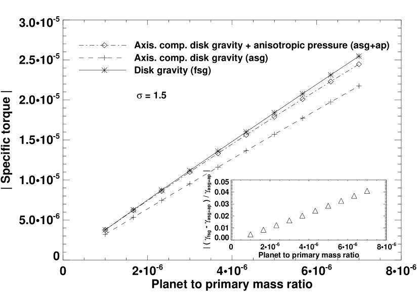
Figure 12: Specific torque as a function of the planet to primary mass ratio. Calculations obtained with the anisotropic pressure model (asg+ap) are compared with axisymmetric self-gravitating calculations (asg) and fully self-gravitating calculations (fsg). The close-up displays the relative difference of the torques between the fsg and asg+ap situations. For all these calculations, $Q=8$ at the planet location (the disk mass is $\sim 0.024M_{*}$).

5 Corotation torque issues

Hitherto, we have considered an initial surface density profile scaling with $r^{-3/2}$, inducing a negligible vortensity gradient, hence a negligible corotation torque. This assumption ensured that the torques derived from our calculations accounted only for the differential Lindblad torque. It enabled a direct comparison with analytical expectations focusing on the differential Lindblad torque. We release this assumption and evaluate the impact of the disk self-gravity on the corotation torque $\Gamma_{\rm C}$, in the linear regime. For a disk without self-gravity, $\Gamma_{\rm C}$ can be estimated by the horseshoe drag expression (Masset et al., 2006a), which reads (Ward, 1991, 1992; Masset, 2001)

$$\Gamma_{\rm C}=\frac{3}{4}x_{s}^{4}\,\Omega^{2}(r_{c})\,\Sigma(r_{c})\left[\frac{d\ln(\Sigma/B)}{d\ln r}\right]_{r=r_{c}},$$ (23)

where $x_{s}$ is the half-width of the horseshoe region, $r_{c}$ denotes the corotation radius, and $B=(2r)^{-1}d(r^{2}\Omega)/dr$ is half the vertical component of the flow vorticity. We denote by $\Gamma_{\rm C,asg}$, $\Gamma_{\rm C,asg+ap}$, and $\Gamma_{\rm C,fsg}$ the corotation torques in the asg, asg+ap, and fsg situations. The same quantities without the C subscript refer to the total torque in the corresponding situation.

We performed the same set of asg, asg+ap and fsg calculations as in section 4.1, but with a flat initial surface density profile (we vary the planet to primary mass ratio $q$, for $Q=8$). An additional nog calculation was also performed for $q=5\times 10^{-6}$. The results of these calculations are displayed in Fig. 13. The torques of the nog and asg calculations are hardly distinguishable, their relative difference being $\sim 2$ %, similarly as in section 3.2.1, where $\sigma=1.5$. This difference should therefore be attributed to the differential Lindblad torque rather than to the corotation torque. It confirms that the corotation torque is not altered by the axisymmetric component of the disk gravity.

Furthermore, the torques of the fsg runs are significantly larger than those of the asg+ap runs. Their relative difference varies from $\sim 11$ % to $\sim 17$ %. We do not expect this difference to arise from the differential Lindblad torque, despite the change of $\sigma$. The differential Lindblad torques should therefore differ from $\sim 0.4$ % to $\sim 4$ %, as for $\sigma=1.5$ (close-up of Fig. 12). This reveals that the fsg situation, or the asg+ap situation, or both, boosts the (positive) corotation torque.

We expect in fact the asg+ap situation to enhance the corotation torque. Masset et al. (2006a) have estimated $x_{s}$ for a disk without self-gravity, in the linear regime. Their estimate reads $x_{s}\approx 1.16r_{p}\sqrt{q/h}$. In the limit where the planet mass vanishes, a fluid element on a horseshoe separatrix has a circular trajectory and is only sensitive to the azimuthal gradient of the disk pressure. The above estimate of $x_{s}$ therefore holds for an asg+ap calculation if one substitutes $h$ with $\sqrt{1-\alpha}\,h$, which we checked by a streamline analysis. Thus, we expect the anisotropic pressure model to slightly increase the half-width of the horseshoe zone, thereby increasing the corotation torque as

$$\Gamma_{\rm C,asg+ap}=\frac{\Gamma_{\rm C,asg}}{1-\alpha},$$ (24)

with $\Gamma_{\rm C,asg}$ given by Eq. (23), and $\alpha=\beta/Q$.

To investigate whether the fsg situation also increases the corotation torque, we evaluate the quantity $(\Gamma_{\rm C,fsg}-\Gamma_{\rm C,asg})/\Gamma_{\rm C,asg}$, which can be recast as

$$\frac{\Gamma_{\rm C,fsg}-\Gamma_{\rm C,asg}}{\Gamma_{\rm C,asg}}=\frac{\Gamma_{\rm C,fsg}-\Gamma_{\rm C,asg+ap}}{\Gamma_{\rm C,asg}}+\frac{\Gamma_{\rm C,asg+ap}-\Gamma_{\rm C,asg}}{\Gamma_{\rm C,asg}}.$$ (25)

Using Eq. (24), the second R.H.S. of Eq. (25) reads $\alpha/(1-\alpha)$, and is $\sim 8.4$ %. Moreover, for the sake of simplicity, we neglect the relative change of the differential Lindblad torques. This assumption is grounded for the smallest planet masses that we consider, for which, as stated above, this change does not exceed $\sim 1$ %. The first R.H.S. of Eq. (25) therefore reads $(\Gamma_{\rm fsg}-\Gamma_{\rm asg+ap})/\Gamma_{\rm C,asg}$. The quantity $\Gamma_{\rm C,asg}$ can be connected with $\Gamma_{\rm asg}$, using the estimate of Tanaka et al. (2002) for a flat surface density profile. This connection is motivated by the fact that both the differential Lindblad torque, and the corotation torque are almost identical in the nog and asg situations. This leads to $\Gamma_{\rm C,asg}\approx-1.56\Gamma_{\rm asg}$. Eq. (25) finally reads

$$\frac{\Gamma_{\rm C,fsg}-\Gamma_{\rm C,asg}}{\Gamma_{\rm C,asg}}=-\frac{\Gamma_{\rm fsg}-\Gamma_{\rm asg+ap}}{1.56\,\Gamma_{\rm asg}}+\frac{\alpha}{1-\alpha}.$$ (26)

This ratio is displayed in the close-up of Fig. 13. It shows that the fsg situation slightly enhances the corotation torque, but this enhancement does not exceed $\sim 4.5$ % for the highest planet mass that we consider. For the smallest planet masses, it is negligible with respect to the increase of the corotation torque triggered by the asg+ap situation. Thus, the large difference between the torques of the asg+ap and fsg calculations can be exclusively accounted for by the boost of the corotation torque in the asg+ap situation.

The slight increase of the corotation torque in the fsg calculations should be compared to that of the differential Lindblad torque, which typically amounts to $\sim 17$ % (for $\sigma=1.5$, see Fig. 12). This comparison indicates that the disk self-gravity does hardly change, if at all, the corotation torque.

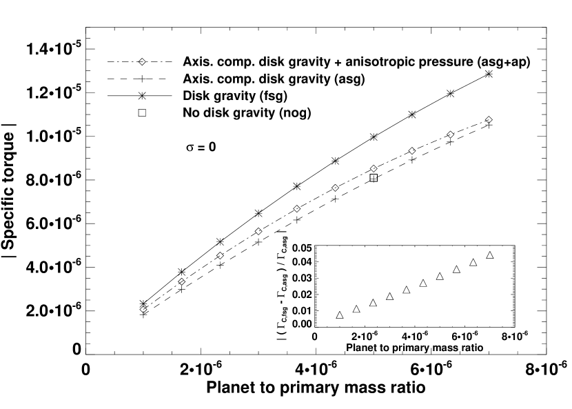
Figure 13: Specific torque as a function of the planet to primary mass ratio, for a flat initial surface density profile. The square corresponds to an additional nog calculation performed with $q=5\times 10^{-6}$. The close-up displays the relative difference of the corotation torques between the asg and fsg situations (see text and Eq. (26)).

6 Concluding remarks

The present work investigates the impact of the disk self-gravity on the type I migration. We show that the assumption customarily used in planet-disk calculations, namely a planet freely migrating in a disk without self-gravity, can lead to a strong overestimate of the migration rate. We provide a simple evaluation of this overestimate (Fig. 5). The drift rate can be overestimated by as much as a factor of two. Such a factor is inappropriate for the accurate calculation of migration rates, which is the main motivation of many recent studies of planet-disk interactions. The planet and the disk must therefore orbit within the same potential to yield unbiased estimates of the drift rate. Avoiding a spurious shift of resonances may be even more crucial in a non-barotropic situation. In this case, the corotation torque depends strongly upon the distance between orbit and corotation (Baruteau & Masset, 2008), so that an ill-located corotation would yield meaningless drift rates.

The inclusion of the disk self-gravity in our calculations confirms that the disk gravity accelerates type I migration. We solve the contradiction between the statements of Nelson & Benz (2003a, b) and Pierens & Huré (2005) regarding the impact of the disk self-gravity on the migration rate. The increase of the differential Lindblad torque due to the disk gravity is typically one order of magnitude smaller than the spurious one induced by a planet freely migrating in a non self-gravitating disk. We provide a simple evaluation of this torque increase (Fig. 8), which depends only on the Toomre parameter at the planet location, whatever the mass distribution of the whole disk. Furthermore, we argue that it can be entirely accounted for by a shift of the Lindblad resonances, and be modeled with an anisotropic pressure tensor. This model succeeds in reproducing the differential Lindblad torque of a self-gravitating calculation, but increases the corotation torque. This model enables us to conclude that there is no significant impact of the disk self-gravity on the corotation torque, in the linear regime.

In a future work, we will extend our study beyond the linear regime. Preliminary calculations show that, regardless of the planet mass, the disk gravity speeds up migration. It would also be of interest to extend this study in three-dimensions. In the linear regime, we do not expect the torque relative increase due to the disk gravity to be altered in three-dimensions. However, three-dimensional calculations, involving the gas self-gravity, should be of considerable relevance for intermediate planet masses when a circumplanetary disk builds up, in particular to assess the frequency of type III migration.

Appendix A Expressions of $g_{r}$ and $g_{\varphi}$

In this section, we give the expressions of the radial and azimuthal self-gravitating accelerations $g_{r}$ and $g_{\varphi}$, smoothed over the softening length $\varepsilon_{\rm sg}$. We use the variables ($u=\log(r/r_{\rm min})$, $\varphi$), where $r_{\rm min}$ denotes the inner edge radius of the grid. With this set of coordinates, $g_{r}(u,\varphi)$ reads

$$\left.g_{r}(u,\varphi)\right.= - Ge^{-u/2}\,\int_{0}^{u_{\rm max}}\int_{0}^{2\pi}S_{r}(u^{{}^{\prime}},\varphi^{{}^{\prime}})\,K_{r}(u-u^{{}^{\prime}},\varphi-\varphi^{{}^{\prime}})\,du^{{}^{\prime}}d\varphi^{{}^{\prime}}$$ (A1)

$$+ G\Sigma(u,\varphi)K_{r}(0,0)\Delta u\Delta\varphi,$$

where $S_{r}$ and $K_{r}$ are defined as

$$S_{r}(u,\varphi)=\Sigma(u,\varphi)~{}e^{u/2}~{}~{}~{}~{}\rm and~{}~{}~{}~{}K_{r}(u,\varphi)=\frac{1+B^{2}-e^{-u}\cos(\varphi)}{\{2(\cosh(u)-\cos(\varphi))+B^{2}e^{u}\}^{3/2}}.$$ (A2)

In Eqs. (A1) and (A2), $G$ denotes the gravitational constant, $u_{\rm max}=\log(r_{\rm max}/r_{\rm min})$ with $r_{\rm max}$ the outer edge radius of the grid, $\Sigma$ is the disk surface density, $\Delta u$ and $\Delta\varphi$ are the mesh sizes, $K_{r}(0,0)=1/B$ and $B=\varepsilon_{\rm sg}/r$. Since $\varepsilon_{\rm sg}\propto r$ (see section 2.2.1), $B$ is uniform over the grid. The second term on the R.H.S. of Eq. (A1) is an additional corrective term that ensures the absence of radial self-force. Similarly, $g_{\varphi}(u,\varphi)$ reads

$$g_{\varphi}(u,\varphi)=-Ge^{-3u/2}~{}\int_{0}^{u_{\rm max}}\int_{0}^{2\pi}S_{\varphi}(u^{{}^{\prime}},\varphi^{{}^{\prime}})~{}K_{\varphi}(u-u^{{}^{\prime}},\varphi-\varphi^{{}^{\prime}})~{}du^{{}^{\prime}}d\varphi^{{}^{\prime}},$$ (A3)

with $S_{\varphi}$ and $K_{\varphi}$ given by

$$S_{\varphi}(u,\varphi)=\Sigma(u,\varphi)~{}e^{3u/2}~{}~{}~{}~{}\rm and~{}~{}~{}~{}K_{\varphi}(u,\varphi)=\frac{\sin(\varphi)}{\{2(\cosh(u)-\cos(\varphi))+B^{2}e^{u}\}^{3/2}}.$$ (A4)

In the particular case where only the axisymmetric component of the disk self-gravity is accounted for, which involves the axisymmetric component of the disk surface density $\overline{\Sigma}(u)=(2\pi)^{-1}\int_{0}^{2\pi}\Sigma(u,\varphi)d\varphi$, $g_{\varphi}$ cancels out and

$$g_{r}(u)=-Ge^{-u/2}\,\int_{0}^{u_{\rm max}}\overline{S_{r}}(u^{{}^{\prime}})\,\widetilde{K_{r}}(u-u^{{}^{\prime}})\,du^{{}^{\prime}}+G\overline{\Sigma}(u)\Delta u\widetilde{K_{r}}(0),$$ (A5)

where $\overline{S_{r}}(u)=(2\pi)^{-1}\int_{0}^{2\pi}S_{r}(u,\varphi)d\varphi$ and $\widetilde{K_{r}}(u)=\int_{0}^{2\pi}K_{r}(u,\varphi)d\varphi$.

Appendix B Relative difference of the torques between the free and fixed situations (without disk gravity)

We denote by $\delta\Gamma$ the difference of the one-sided Lindblad torques between the free and fixed cases. This difference can be written as

$$\delta\Gamma=\sum_{m}\left(\frac{\partial T}{\partial x}\right)_{x_{L}}\delta x,$$ (B1)

where $x=r-r_{p}$, $\delta x$ is the shift of the Lindblad resonances induced by the free case, $T$ is the $m^{\rm th}$ Fourier component of the one-sided Lindblad torque (see e.g. Ward, 1997, or Eq. (14)), and $x_{L}$ is the location of the Lindblad resonances in the fixed situation:

$$x_{L}=\frac{2}{3}\epsilon\frac{\sqrt{1+\xi^{2}}}{\xi}hr_{p},$$ (B2)

with $\xi=mh$, $\epsilon=+1$ for outer resonances, $\epsilon=-1$ for inner resonances. Approximating the summation over $m$ as an integral over $\xi$, Eq. (B1) can be recast as

$$\delta\Gamma=\int(\partial_{x}T/T)\times T\times\delta x\,d\xi.$$ (B3)

In Eq. (B3), $T$ depends on $x$ through the square of the forcing function $\Psi$, which is usually approximated as a function of the Bessel functions $K_{0}$ and $K_{1}$ (see e.g. Ward, 1997, or Eq. (15)). Furthermore, $\Psi(x,\xi)$ can be approximated as $hr_{p}/|x|\xi$, to within a numerical factor of the order of unity (Abramowitz & Stegun, 1972). Thus, $T\propto x^{-2}$ and $\partial_{x}T/T\propto x^{-1}$. At the location of Lindblad resonances, given by Eq. (B2), this yields $\partial_{x}T/T\propto\epsilon h^{-1}$. Moreover, $T\propto\epsilon\Sigma_{p}h^{-3}$. The shift $\delta x$, which has same sign for inner and outer Lindblad resonances, scales with $\Sigma_{p}$. The difference of the differential Lindblad torques is eventually obtained by summing Eq. (B3) at inner and outer Lindblad resonances,

$$\delta\Gamma_{\rm ILR}+\delta\Gamma_{\rm OLR}\propto\Sigma_{p}h^{-1}\int(T_{\rm OLR}-T_{\rm ILR})d\xi\propto\Sigma_{p}h^{-1}\times\Sigma_{p}h^{-3}\propto\Sigma_{p}^{2}h^{-4}.$$ (B4)

Since the differential Lindblad torque scales with $\Sigma_{p}h^{-2}$, the relative difference of the differential Lindblad torques between the free and fixed cases scales with $\Sigma_{p}h^{-2}$, hence with $(Qh)^{-1}$.

Appendix C Relative difference of the torques with and without disk gravity

The calculation of the difference $\delta\Gamma$ of the one-sided Lindblad torques between the fully self-gravitating and non-gravitating situations is similar to the one derived in Appendix B. The difference $\delta\Gamma$ is given again by Eq. (B3), where $\delta x$ is this time the shift induced by the fsg situation. This shift has an opposite sign at inner and outer Lindblad resonances: $\delta x\propto\epsilon\Sigma_{p}$ (see the $\delta R_{2}$ expression of PH05, or skip to Eq. (12) where however $x=(r-r_{p})/hr_{p}$). Furthermore, assuming that the expression of $T$ given by Eq. (14) can be applied for a self-gravitating disk (Goldreich & Tremaine, 1979), we still have $\partial_{x}T/T\propto\epsilon h^{-1}$. Since the differential Lindblad torque scales with $\Sigma_{p}h^{-2}$, we find

$$\delta\Gamma_{\rm ILR}+\delta\Gamma_{\rm OLR}\propto\Sigma_{p}h^{-1}\int(T_{\rm OLR}+T_{\rm ILR})d\xi\propto\Sigma_{p}h^{-1}\times\Sigma_{p}h^{-2}\propto\Sigma_{p}^{2}h^{-3}.$$ (C1)

The relative difference of the differential Lindblad torques between the fsg and nog cases therefore scales with $\Sigma_{p}h^{-1}$, hence with $Q^{-1}$.

Appendix D Numerical and analytical shifts of Lindblad resonances induced by the disk self-gravity

We studied in section 3.3.2 the relative difference of the torques between the fsg and nog situations. In particular, we find that our calculations with $\varepsilon=0.1H(r_{p})$, which matches the mesh resolution in the planet vicinity, display a relative difference that is stronger than the one obtained with the estimate of PH05, which however does not involve a softening parameter. We give hereafter more insight into this result.

We propose to evaluate for each azimuthal wavenumber $m$ the shift of the Lindblad resonances induced by our fsg calculations, and compare it with its theoretical expression given by Eq. (12). This theoretical expression predicts that the shifts at inner and outer resonances are of opposite sign, their absolute value, which we denote by $\delta x_{\rm th,m}$, being identical. We furthermore denote $\delta x_{\rm num,m}$ the shift (in absolute value) inferred from our calculations, and $\Gamma^{i}_{\rm fsg,m}$ ($\Gamma^{o}_{\rm fsg,m}$) the $m^{\rm th}$ Fourier component of the inner (outer) Lindblad torque of a fsg calculation. We use similar notations for a nog calculation, and we drop hereafter the $m$ subscripts for the sake of legibility. A first-order expansion yields

$$\Gamma^{i}_{\rm fsg}=\Gamma^{i}_{\rm nog}+\partial_{x}\Gamma^{i}_{\rm nog}\,\delta x_{\rm num}~{}~{}~{}~{}{\rm and}~{}~{}~{}~{}\Gamma^{o}_{\rm fsg}=\Gamma^{o}_{\rm nog}-\partial_{x}\Gamma^{o}_{\rm nog}\,\delta x_{\rm num}.$$ (D1)

To estimate the quantities $\partial_{x}\Gamma^{i}_{\rm nog}$ and $\partial_{x}\Gamma^{o}_{\rm nog}$, we performed an additional nog calculation, mentioned as nogo calculation, for which we imposed a slight, known shift of the resonances. This was done by fixing the planet’s angular velocity at $\Omega_{p}-\delta\Omega_{p}$, with $\delta\Omega_{p}=10^{-5}\Omega_{p}$. This slight decrease of the planet’s angular velocity, with respect to the nog situation, implies an outward shift of inner and outer Lindblad resonances that reads $\delta x_{\rm o}=(2\delta\Omega_{p})/(3h\Omega_{p})$, expression that is independent of $m$. With similar notations as before for the nogo calculation, and using again a first-order expansion, we have

$$\Gamma^{i}_{\rm nogo}=\Gamma^{i}_{\rm nog}+\partial_{x}\Gamma^{i}_{\rm nog}\,\delta x_{\rm o}~{}~{}~{}~{}{\rm and}~{}~{}~{}~{}\Gamma^{o}_{\rm nogo}=\Gamma^{o}_{\rm nog}+\partial_{x}\Gamma^{o}_{\rm nog}\,\delta x_{\rm o}.$$ (D2)

Combining Eqs. (D1) and (D2), we are finally left with

$$\delta x_{\rm num}=\frac{(\Gamma^{i}_{\rm fsg}-\Gamma^{o}_{\rm fsg})-(\Gamma^{i}_{\rm nog}-\Gamma^{o}_{\rm nog})}{(\Gamma^{i}_{\rm nogo}+\Gamma^{o}_{\rm nogo})-(\Gamma^{i}_{\rm nog}+\Gamma^{o}_{\rm nog})}\times\delta x_{\rm o}.$$ (D3)

We plot in Fig. 14 the ratio $\delta x_{\rm num}/\delta x_{\rm th}$ as a function of the azimuthal wavenumber $m$, for $\Sigma_{p}=2\times 10^{-3}$ ($Q\sim 8$). We first comment that the ratio is negative for $m\leq 6$, positive beyond, with a divergent behavior at the transition. We checked that this behavior is caused by a change of sign of the denominator of Eq. (D3), which is negative for $m\leq 6$ and positive beyond. Furthermore, the ratio $\delta x_{\rm num}/\delta x_{\rm th}$ is significantly greater than unity for $m$ ranging from $\sim 7$ to $\sim 20$, that is for the dominant Lindblad resonances. Differently stated, the dominant Lindblad resonances are more shifted by our calculations than analytically expected by PH05, which explains why the torque enhancement is more important with our calculations.

Beyond, the ratio is close to unity for a rather large range of high $m$-values. This confirms that for high values of $m$ the WKB approximation yields analytical estimates that are in good agreement with the results of numerical simulations. However, since our calculations involve a softening parameter, the ratio does not converge when increasing $m$, and slowly tends to zero. We checked that the value of $m$ for which the ratio becomes lower than unity increases when decreasing the softening length. This explains why the torque enhancement is increasingly important at smaller softening length, as inferred from Fig. 10.

Figure 14: Ratio of $\delta x_{\rm num}$, the shift of Lindblad resonances obtained with our fsg calculations (see Eq. (D3)), and of $\delta x_{\rm th}$, its analytically expected value (see Eq. (12)).

References

- Abramowitz & Stegun (1972) Abramowitz, M. & Stegun, I. A. 1972, Handbook of Mathematical Functions (Handbook of Mathematical Functions, New York: Dover, 1972)
- Baruteau & Masset (2008) Baruteau, C. & Masset, F. 2008, ApJ, 672, 1054
- Binney & Tremaine (1987) Binney, J. & Tremaine, S. 1987, Galactic dynamics (Princeton, NJ, Princeton University Press, 1987, 747 p.)
- Boss (2005) Boss, A. P. 2005, ApJ, 629, 535
- Crida et al. (2006) Crida, A., Morbidelli, A., & Masset, F. 2006, Icarus, 181, 587
- de Val-Borro et al. (2006) de Val-Borro, M., Edgar, R. G., Artymowicz, P., Ciecielag, P., Cresswell, P., D’Angelo, G., Delgado-Donate, E. J., Dirksen, G., Fromang, S., Gawryszczak, A., Klahr, H., Kley, W., Lyra, W., Masset, F., Mellema, G., Nelson, R. P., Paardekooper, S.-J., Peplinski, A., Pierens, A., Plewa, T., Rice, K., Schäfer, C., & Speith, R. 2006, MNRAS, 695
- Goldreich & Tremaine (1979) Goldreich, P. & Tremaine, S. 1979, ApJ, 233, 857
- Huré & Pierens (2006) Huré, J.-M. & Pierens, A. 2006, in SF2A-2006: Semaine de l’Astrophysique Francaise, ed. D. Barret, F. Casoli, G. Lagache, A. Lecavelier, & L. Pagani, 105–+
- Masset (2000a) Masset, F. 2000a, A&AS, 141, 165
- Masset (2000b) Masset, F. S. 2000b, in Astronomical Society of the Pacific Conference Series, Vol. 219, Disks, Planetesimals, and Planets, ed. G. Garzón, C. Eiroa, D. de Winter, & T. J. Mahoney, 75–+
- Masset (2001) Masset, F. S. 2001, ApJ, 558, 453
- Masset et al. (2006a) Masset, F. S., D’Angelo, G., & Kley, W. 2006a, ApJ, 652, 730
- Masset et al. (2006b) Masset, F. S., Morbidelli, A., Crida, A., & Ferreira, J. 2006b, ApJ, 642, 478
- Mayor & Queloz (1995) Mayor, M. & Queloz, D. 1995, Nature, 378, 355
- Menou & Goodman (2004) Menou, K. & Goodman, J. 2004, ApJ, 606, 520
- Narayan et al. (1987) Narayan, R., Goldreich, P., & Goodman, J. 1987, MNRAS, 228, 1
- Nelson & Benz (2003a) Nelson, A. F. & Benz, W. 2003a, ApJ, 589, 556
- Nelson & Benz (2003b) —. 2003b, ApJ, 589, 578
- Paardekooper & Mellema (2006) Paardekooper, S.-J. & Mellema, G. 2006, A&A, 459, L17
- Pierens & Huré (2005) Pierens, A. & Huré, J.-M. 2005, A&A, 433, L37
- Sellwood (1987) Sellwood, J. A. 1987, ARA&A, 25, 151
- Tanaka et al. (2002) Tanaka, H., Takeuchi, T., & Ward, W. R. 2002, ApJ, 565, 1257
- Tanigawa & Lin (2005) Tanigawa, T. & Lin, D. N. C. 2005, in Protostars and Planets V, 8466–+
- Toomre (1964) Toomre, A. 1964, ApJ, 139, 1217
- van Leer (1977) van Leer, B. 1977, Journal of Computational Physics, 23, 276
- Ward (1991) Ward, W. R. 1991, in Lunar and Planetary Institute Conference Abstracts, 1463–+
- Ward (1992) Ward, W. R. 1992, in Lunar and Planetary Institute Conference Abstracts, 1491–+
- Ward (1997) Ward, W. R. 1997, Icarus, 126, 261