Dependence of the BALQSO fraction on Radio Luminosity

Abstract

We find that the fraction of classical Broad Absorption Line quasars (BALQSOs) among the FIRST radio sources in the Sloan Data Release 3, is $20.5^{+7.3}_{-5.9}$% at the faintest radio powers detected ($L_{\rm 1.4GHz}\sim 10^{32}\,{\rm erg\,s^{-1}}$), and rapidly drops to $\lesssim 8$% at $L_{\rm 1.4\,GHz}\sim 3\times 10^{33}\,{\rm erg\,s^{-1}}$. Similarly, adopting the broader Absorption Index (AI) definition of Trump et al. (2006) we find the fraction of radio BALQSOs to be $44^{+8.1}_{-7.8}$% reducing to $23.1^{+7.3}_{-6.1}$% at high luminosities. While the high fraction at low radio power is consistent with the recent near-IR estimates by Dai et al. (2008), the lower fraction at high radio powers is intriguing and confirms previous claims based on smaller samples. The trend is independent of the redshift range, the optical and radio flux selection limits, or the exact definition of a radio match. We also find that at fixed optical magnitude, the highest bins of radio luminosity are preferentially populated by non-BALQSOs, consistent with the overall trend. We do find, however, that those quasars identified as AI-BALQSOs but not under the classical definition, do not show a significant drop in their fraction as a function of radio power, further supporting independent claims for which these sources, characterized by lower equivalent width, may represent an independent class with respect to the classical BALQSOs. We find the balnicity index, a measure of the absorption trough in BALQSOs, and the mean maximum wind velocity to be roughly constant at all radio powers. We discuss several plausible physical models which may explain the observed fast drop in the fraction of the classical BALQSOs with increasing radio power, although no one is entirely satisfactory. A strictly evolutionary model for the BALQSO and radio emission phases requires a strong fine-tuning to work, while a simple geometric model, although still not capable of explaining polar BALQSOs and the paucity of FRII BALQSOs, is statistically successful in matching the data if part of the apparent radio luminosity function is due to beamed, non-BALQSOs.

1. Introduction

It is a main theme in Active Galactic Nuclei (AGN) studies to describe various AGN phenomena within coherent schemes. The broad absorption line quasars (BALQSOs) and radio quasars (RQs) are both subsamples of quasars, where BALQSOs exhibit blue-shifted rest-frame ultra-violet absorption troughs (e.g., Weymann et al. 1991) and RQs are characterized by their radio emission (e.g., Matthews & Sandage 1963; Schmidt 1963; Kellermann et al. 1989). The fractions of BALQSOs and RQs are the subjects of many studies (e.g., Weymann et al. 1991; Hewett & Foltz 2003; White et al. 2007). Recently, Dai et al. (2007, DSS hereafter), adopting the classical Balnicity Index (BI) definition (Weymann et al. 1991) which selects as BALQSOs those sources with absorption troughs wider than 2000 ${\rm km\,s^{-1}}$, obtained an intrinsic BALQSO fraction of $(20\pm 0.2)\%$ using the BALQSOs detected in the Two Micron All Sky Survey (2MASS) and in the Sloan Digital Sky Survey (SDSS) Data Release 3 (DR3) BALQSO catalog of Trump et al. (2006). DSS showed that the BALQSO fraction calculated in the infrared is significantly higher by a factor of $\sim 2$ than that inferred from optical samples alone. Since the infrared bands are less affected by selection effects due to dust extinction and absorption troughs, DSS concluded that the infrared fractions should be much closer to the true intrinsic fractions of BALQSOs. The intrinsic fraction from DSS is consistent with the early estimate by Hewett & Foltz (1993) inferred by directly correcting the obscuration effects in the optical bands, and subsequent analysis using similar methods by Knigge et al. (2008). In addition, such a a high intrinsic fraction has been recently confirmed by Maddox et al. (2008), from a deeper sample constructed from the UKIRT Infrared Deep Sky Survey Early Data Release, which probes about three magnitudes fainter than 2MASS. DSS also showed that an intrinsic BALQSO fraction of 43% is found when adopting the broader Absorption Index (AI) classification by Trump et al. (2006) which identifies BALQSOs as those quasars with absorption troughs which have an equivalent width (measured between 0 and 29000 ${\rm km\,s^{-1}}$) greater than 1000 ${\rm km\,s^{-1}}$. The validity of the latter definition has however been recently questioned (e.g., Ganguly et al. 2007; Knigge et al. 2008), and in this paper we will therefore discuss results adopting both definitions.

On the other hand, recent results on the fraction of RQs in optical samples are between 10–20%, depending on the definition (e.g., Sikora et al. 2007 and references therein). In several studies, the RQ fraction is found to depend on the redshift and optical luminosity (e.g., Jiang et al. 2007). In general, constraining the intrinsic fractions of BALQSOs and RQs in large, complete quasar samples, is important for understanding the nature of these phenomena such as their efficiency and/or black hole spin distributions (e.g., Murray et al. 1995; Sikora et al. 2007; Shankar et al. 2008b), and helping constrain AGN and galaxy evolutionary models (e.g., King 2003; Croton et al. 2006; Granato et al. 2006; Hopkins et al. 2006; Lapi et al. 2006; Shankar et al. 2006).

The fraction of BALQSOs in RQs is particularly interesting as it may further constrain which quasar sub-samples are caused by geometrical viewing effects and which are caused by evolutionary effects, as well as provide additional clues on the nature and connections between these two apparently disconnected quasar phenomena. In a pioneer study, Stocke et al. (1992) found no evidence for luminous radio sources among 68 BALQSOs. In a sample of 255 radio sources in the Large Bright QSO Survey, Francis et al. (1993) noted that the fraction of radio-moderate quasars with BAL features was significantly higher than in the radio-quiet population. Brotherton et al. (1998) found five BALQSOs in a complete sample of 111 QSO candidates also detected in the NRAO VLA Sky Survey. Using the FIRST Bright Quasar Survey, Becker et al. (2000) found 29 BALQSOs, about 14–18% of their total sample, suggesting a frequency of BALQSOs significantly greater than the typical $\sim$ 10% inferred from optically selected samples at that time. Within the small sample, they also found that the BALQSO fraction has a complex dependence on radio loudness. However, the trend they found was driven by the 11 low-ionization BALQSOs, whereas the 18 high-ionization BALQSOs were slightly under-represented at high radio loudness, but at a statistically insignificant level. With a larger sample of 25 high-ionization and 6 low-ionization BALQSOs selected from an extension of the FIRST Bright Quasar Survey to the South Galactic cap and to a fainter optical magnitude limit, Becker et al. (2001) confirmed the results by Becker et al. (2000) of a steady decrease of the high-ionization BALQSO. Using the Large Bright Quasar Survey, Hewett and Foltz (2003) argued that with a consistent BALQSO definition there is no inconsistency in the BALQSO fractions between optically-selected and radio-selected quasar samples. They also found that “optically-bright BALQSOs are half as likely as non-BALQSOs to be detectable $S_{1.4\rm GHz}\gtrsim 1$ mJy as radio sources”. In this paper, we combined the SDSS-DR3 BALQSO sample (Trump et al. 2006), containing more than 4,000 BALQSOs, with the FIRST survey data (Becker et al. 1995) to study the fraction of BALQSOs in the radio detected sample.

2. The Data

The parent sample for the Trump et al. (2006) BALQSO catalog is the SDSS DR3 quasar catalog (Schneider et al. 2005). Data were taken in five broad optical bands ($ugriz$) over about 10,000 deg² of the high Galactic latitude sky. The majority of quasars were selected for spectroscopic followup by SDSS based on their optical photometry. In particular, most quasar candidates were selected by their location in the low-redshift ($z\lesssim 3$) $ugri$ color cube with its $i$-magnitude limit of 19.1. A second higher redshift $griz$ color cube was also used with a fainter $i$-magnitude limit of 20.2. Following DSS, we focus on redshift range of $1.7\leq z\leq 4.38$, where BALQSOs are identified by C iv absorption in the SDSS spectra. In the following we present results using both the AI and BI definitions for BALQSOs.

The DR3 quasar catalog by Schneider et al. (2005) also provides the radio flux for those sources which have a counterpart within 2${}^{\prime\prime}\,$in the FIRST catalog (Becker et al. 1995). However, we use the integrated flux density observed at 1.4 GHz as listed in the FIRST catalog to calculate the specific luminosity emitted at 1.4 GHz, $L_{1.4{\rm\,GHz}}$, via the relation

$$L_{1.4{\rm GHz}}=\frac{f_{\rm int}\times 10^{-26}}{(1+z)^{1-\alpha}}4\pi D_{L}^{2}{\rm\,erg\,s^{-1}\,Hz}^{-1}\,,$$ (1)

where $f_{\rm int}$ is the integrated flux density in mJy, $\alpha$ is the spectral index (i.e., $f(\nu)\propto\nu^{-\alpha}$), and $D_{L}$ is the luminosity distance in cm as calculated from the redshift setting $\Omega_{m}=0.3$, $\Omega_{\rm\Lambda}=0.7$ and $h=0.7$. We assume $\alpha=0.7$, which is intermediate of the typical range for radio jets (Bridle & Perley 1984). Our results do not qualitatively change if we assume either $\alpha=0.5$ or $\alpha=1.0$.

According to Schneider et al. (2005), while only a small minority of FIRST-SDSS matches are chance superpositions, a significant fraction of the DR3 sources are extended radio sources. Therefore the FIRST catalog position for the latter may differ by more than 2${}^{\prime\prime}\,$from the optical position. To perform a comprehensive study of the BALQSO radio fraction, we built a full FIRST-SDSS cross-correlation catalog, containing all the detected radio components within 30${}^{\prime\prime}\,$of a optical quasar. As our reference, following Schneider et al. (2005), we primarily present results for the FIRST-SDSS catalog with radio counterparts defined within 2${}^{\prime\prime}\,$, which contains a total of 652 radio sources, out of which 78 are BALQSOs, about three times the sample used by Becker et al. (2001) for BALQSOs. We will discuss results obtained by enlarging the radio matches to 5${}^{\prime\prime}\,$. In addition, many of the optical sources in SDSS are associated to more than one radio component in FIRST within 30${}^{\prime\prime}\,$, as expected if these sources are extended with jets and/or lobes separated from the central source. We will therefore discuss results after the inclusion of BALQSO sources characterized by multiple radio components, for which we use the sum of the flux densities as a proxy for the total radio luminosity of the source.

Finally, we also stress that FIRST efficiently identifies radio matches to optically-selected quasars. By cross-correlating SDSS with the large radio NRAO VLA Sky Survey (Condon et al. 1998), Jiang et al. (2007) found in fact that only $\sim$ 6% of the matched quasars were not detected by FIRST. Most of these sources have offsets more than 5${}^{\prime\prime}\,$and are uniformly distributed in luminosity thus not altering the main conclusions of this paper.

3. Results

3.1. The Radio fraction of BALQSOs

The solid crosses in the left panel of Figure 1 show the fraction

$$f_{\rm BAL}=\frac{N_{\rm BAL,RADIO}}{N_{\rm RADIO}}\,,$$ (2)

as a function of radio luminosity, where $N_{\rm RADIO}$ is the total number of RQs detected in SDSS and $N_{\rm BAL,RADIO}$ is the number of RQs which are also classified as BALQSOs. For this plot we only used the “complete” SDSS optical sample with apparent optical magnitude $m_{i}\leq 19.1$. The bins in $L_{1.4{\rm\,GHz}}$ were created adaptively starting from low radio luminosities by requiring a statistically significant sub-sample of 50 quasars in each bin of luminosity. In each bin we used the binomial theorem to estimate $f_{\rm BAL}$ along with its $\pm 1\sigma$ confidence levels (e.g., Gehrels et al. 1986).

The first important result of our analysis is the high fraction of classical (BI) BALQSOs detected at low radio powers. The BALQSO fraction of $20^{+7.3}_{-5.9}$% at the faintest radio powers of $L_{1.4{\rm\,GHz}}\lesssim 10^{33}\,{\rm erg\,s^{-1}}$ is in strikingly good agreement with the 20% classical BALQSO occurrence inferred by DSS in the 2MASS-SDSS sample (shown with horizontal, thin-dotted line in Figures 1 and 3). This result further supports and extends the key result discussed in DSS that the detected BALQSO fraction should be closer to the intrinsic one at longer wavelengths, which are gradually less affected by absorption troughs and dust extinction.

The second striking result of our study is that $f_{\rm BAL}$ drops rapidly with increasing radio power to $8.0^{+5.9}_{-3.8}$% at $L_{1.4{\rm\,GHz}}\gtrsim 2\times 10^{33}\,{\rm erg\,s^{-1}}$. This behavior strongly supports some close connection between radio and BALQSO phenomena and, as discussed below, poses serious challenges to simple evolutionary models.

The open symbols with dashed crosses represent the fraction $f_{\rm BAL}$ obtained including all AI-selected BALQSOs. As expected, we get a much larger fraction of BALQSOs within our sample of $44^{+8.1}_{-7.8}$%, in very good agreement with the findings by DSS who found a fraction of 43% AI BALQSOs in 2MASS (thick-dotted line). Even in this case, $f_{\rm BAL}$ presents a very similar behavior as a function of radio luminosity and that we will discuss in § 3.2.

3.2. Robustness of Results

Our results are derived by cross-correlating optical quasars, RQs, and BALQSOs. Therefore it is natural to expect that several issues may affect our conclusions. In this section we carefully analyze the most significant sources of bias which can enter our computations and find that none of these seems to be responsible for the observed $f_{\rm BAL}-L_{1.4{\rm\,GHz}}$ behavior.

We first tested for biases from redshift or luminosity selection effects. When repeating our analysis using only the sources in two redshift bins $1.7\lesssim z\lesssim 2.5$ and, separately, $2.5\lesssim z\lesssim 4.38$, we find very similar trends for the $f_{\rm BAL}$-$L_{1.4{\rm\,GHz}}$ relation.

The completeness of the Schneider et al. (2005) quasar sample has been studied in detail by Vanden Berk et al. (2005), who estimate a total completeness of 89.3% down to $m_{i}=19.1$. We do not expect the behavior of $f_{\rm BAL}$ to be severely influenced by these mild incompleteness effects. As extensively discussed (e.g., Cirasuolo et al. 2003; Shankar et al. 2008b, and references therein), the radio and optical luminosities are correlated with a large observed scatter. Therefore, incompleteness effects in the optical sample will, on average, induce similar effects in the numerator and denominator of equation (2), given the extended distribution of optical sources at fixed radio luminosity. As an example of the effect of different optical luminosity thresholds on the fraction of BALQSOs, we show the resulting $f_{\rm BAL}$ with no optical magnitude cut in the right panel of Figure 1. This highly incomplete sample in the optical still shows the exact same drop of at least a factor of $\sim 4$ in $f_{\rm BAL}$.

On the other hand, our sample may suffer from selection effects in FIRST. At 3 mJy the completeness of FIRST is about $93$%, decreasing to 75% at 1.5 mJy, and 55% at 1.1 mJy (see Figure 1 in Jiang et al. 2007). To check whether our results were affected by this incompleteness, in Figure 2 we compare the results shown in the left panel of Figure 1 obtained from the full sample (solid crosses), with the sample defined by only those radio sources with $f_{\rm int}>3$ mJy (dashed crosses). This cut in radio flux density ensures the best completeness as possible from FIRST. It is evident that the strong observed drop in $f_{\rm BAL}$ remains unchanged.

As anticipated in § 2, the 2${}^{\prime\prime}\,$cross-correlation sample ensures a secure identification of the core radio power associated to an optical quasar. However, to check for any bias in our results due to incomplete radio identifications in the SDSS DR3 quasar catalog, we recomputed $f_{\rm BAL}$ using the full sample built by matching SDSS and FIRST. The left panel of Figure 3 shows the fraction of BALQSOs with the radio counterpart defined by the nearest source in FIRST within 5${}^{\prime\prime}\,$. The right panel of Figure 3 shows instead the fraction of BALQSOs with at least one radio counterpart within 30${}^{\prime\prime}\,$of the optical source. In both cases we still find $f_{\rm BAL}$ to drop with increasing radio power. These results are actually expected, as a closer inspection revealed that the overall sample of radio-optical sources increases by just $\sim 4$% when including sources within 5${}^{\prime\prime}\,$, out of which only 3 extra BALQSOs are found with respect to our reference sample. The increase is even milder ($\sim 3$%) when the 30${}^{\prime\prime}\,$sources are included, with only 2 extra BALQSOs included in the sample. The paucity of extended radio sources in our sample is in agreement with Gregg et al. (2006) who found only six quasars from the DR3 and FIRST Bright Quasar Survey that exhibit Fanaroff-Riley II-type (FRII) morphologies and BAL properties, with a BI index strongly decreasing with increasing radio loudness.

In Figure 4 we show $f_{\rm BAL}$ as a function of absolute optical magnitude. We do not find significant evidence for any sharp trend of $f_{\rm BAL}$ as a function of $M_{i}$, confirming the results by DSS for the 2MASS sample. This implies that different optical magnitude cuts do not affect $f_{\rm BAL}$ on one hand, and, on the other, implies that the drop in $f_{\rm BAL}$ is mainly a “radio phenomenon”, not linked with the quasar bolometric luminosity. Note that we did not apply any correction in Figure 4 for extinction as was done in DSS, therefore the resulting fractions in the optical are lower than the intrinsic ones (see DSS for details).

The AI sample by Trump et al. (2006) may suffer from a significant contamination of false positives, which the close inspection by Ganguly et al. (2007) found to be about 30% (see also Knigge et al. 2008). To investigate the impact these findings may have on our results we have compared the sample of sources cataloged as BALQSOs using the AI definition, with the sample of BALQSO defined using the classical BI index. The distribution of AI-BALQSOs with radio counterparts as a function of the AI index (open histogram) is compared in the upper left panel of Figure 5 with the distribution of the sources which are also identified as BI-BALQSOs (filled histogram). We find the latter sample strongly peaked at higher AI values, while just the opposite is true for most of the AI-BALQSOs. These findings are fully consistent with the recent results by Knigge et al. (2008) who claim for a well distinct separation for the two BALQSO samples. The upper right panel of Figure 5 plots the fraction of AI- but not BI-identified BALQSOs as a function of radio power: the drop in $f_{\rm BAL}$ with increasing radio power is much less evident for this subclass of sources compared to BI-BALQSOs. These results suggest that AI-BALQSOs are a different class of quasars with respect to the BI-BALQSOs. In the lower right panel of Figure 5 the dashed, dotted and solid lines show the fractions of AI-BALQSOs, AI- but not BI-BALQSOs, and BI-BALQSOs, respectively. This plot confirms that the apparent drop in the AI-BALQSOs with radio power is driven by the behavior in BI-BALQSOs. The lower right panel of Figure 5 shows the cumulative distributions for the different subclasses of BAL and non-BALQSOs, as labeled. We find that the probability that AI but not BI selected BALQSOs are drawn from the same distribution as non-BALQSOs is $P=0.26$, while the probability for being drawn from any other distribution drops by several orders of magnitude.

In Figure 6 we show the distributions of all non-BALQSOs (dashed lines), BI-BALQSOs (solid lines), and AI- but not BI-BALQSOs (dotted lines) as a function of radio luminosity for different bins of absolute optical magnitude, as labeled. These bins were chosen to provide an equal number of BALQSOs in each panel. It is apparent that compared to BI-BALQSOs, both the AI- but not BI-BALQSOs and the non-BALQSO distributions have a greater tendency to populate significantly higher, potentially beamed, radio luminosity bins. This provides further evidence that the trends in $f_{\rm BAL}$ are not a mere consequence of random effects in the radio power distributions of optical quasars. The dashed, dotted, and solid lines in Figure 7 show, respectively, the histograms of the distributions of BI-BALQSOs, AI- but not BI- BALQSOs, and non-BALQSOs as a function of color defined as the difference between absolute $i$-band and AB radio magnitudes listed in Schneider et al. (2005). This plot shows that on average AI- but not BI- BALQSOs, and non-BALQSOs have very similar optical-to-radio distributions while BI-BALQSOs are clearly offset populating lower radio luminosity bins at fixed optical magnitude.

Overall our results show that the classical BALQSO fraction in the radio is as high as inferred from the near-IR and rapidly drops from $\sim 20\%$ to $\lesssim 4\%$ with increasing radio power. This clear trend confirms previous claims by Becker et al. (2001), taking advantage of a sample of $\sim 3$ higher. We conclude that the behavior of $f_{\rm BAL}$ as a function of radio power seems to be an intrinsic, real feature of the radio, BI-BALQSO population, not linked to any significant selection effect. In the following, if not alternatively specified, we will always refer to BALQSOs as those defined through the classical BI definition.

4. Explaining the observed trend

Models aimed at explaining the BALQSO and/or radio fractions, can be broadly divided into two classes: one in which each quasar phase is distinct and characterized by the internal physical evolution undergone by the system, and the other in which all these phenomena co-exist at all times but different source orientations modify the observed balance of one process with respect to another.

4.1. The Evolutionary Model

The results discussed in § 3 seem to pose a serious challenge to “evolutionary” models for BALQSOs. The simple sketch shown in the left panel of Figure 8, represents the basic picture for the evolution of a black hole within its host galaxy (e.g., Kawakatu et al. 2003). The mass of the central black hole, shown as a solid line in the left panel of Figure 8, exponentially grows through gas accretion from the surrounding medium. Initially the whole galaxy, or at least its central region, is buried under optically-thick layers of dust which allow the AGN to be detectable only in those bands that suffer less from obscuration, such as in X-rays (e.g., Ueda et al. 2003). When the black hole becomes sufficiently luminous, it injects enough energy and momentum (e.g., Fabian 1999) into the surrounding medium to disperse the obscuring material. During this blowout phase, the system will be detected as a BALQSO featuring the signatures of strong winds in their spectra, while at later stages it will be observed as an optical, dust-free quasar.

It is still unclear what triggers the radio activity of an AGN (e.g., Sikora et al. 2007), so it is difficult to predict when an optical quasar should become radio-loud (e.g., Blundell & Kuncic 2007; Shankar et al. 2008b). Nevertheless, in pure evolutionary models the radio phase is usually viewed as a brief period within the optical phase as the incidence of RQs in optical samples is rather small, ($\sim 15-20\%$, e.g., Jiang et al. 2007; see also § 1). In this model, our results on $f_{\rm BAL}$ indicate that the radio duty cycle must overlap the boundary between the BALQSO and optical phases, because a significant fraction of optical quasars also emit in radio but are not BALQSOs, and vice versa.

In a pure evolutionary model our result that $f_{\rm BAL}\sim 20\%$ constrains the BALQSO and non-BALQSO phases to last for $\sim$ 20% and 80%, respectively, within the brief radio phase, which is about 15–20% of the total optical quasar lifetime (see left panel of Figure 8). The consistency between the optical and radio BALQSO fractions imposes a coincidence problem, which could be otherwise naturally interpreted in orientation models (§ 4.2). Additionally, the drop in $f_{\rm BAL}$ at high radio powers is difficult to reproduce simply in pure evolutionary models, and thus such models would need to be fine-tuned to explain the drop. One simple explanation for such a trend may be an increasing feedback efficiency with quasar luminosity (e.g., Kelly et al. 2008). The more luminous sources would then be faster in removing the surrounding obscuring medium, shortening the BALQSO phase and consequently inducing a decrease in $f_{\rm BAL}$. However, this model is at variance with the results in Figure 4 and by DSS which show that the BALQSO fraction is constant with optical luminosity.

Gregg et al. (2006) found an absence of BALQSO FRII sources and a drop in the BI index with increasing radio loudness of the sources. They interpreted their results within an evolutionary scheme where a BALQSO occurs in the early stage of a quasar during its emergence from a thick shroud of surrounding dust (see left panel of Figure 8). In this model FRIIs are only seen after most of the obscuring shroud has been removed. Following Gregg et al. (2006) we further probe the constraints for evolutionary models by addressing the coexistence of FRII/BAL sources within our sample. In Figure 9 the open triangles show the fraction of FRII-selected sources within the whole radio sample, while the filled circles refer to the fraction of FRII sources within the BI-selected radio sample. Both samples have been divided into two subgroups with radio luminosities below and above $L_{\rm 1.4GHz}=2\times 10^{33}\,{\rm erg\,s^{-1}\,Hz^{-1}}$. Note that the contamination from random interloping radio sources in the identification of FRII sources is small. The average number of interlopers within 30${}^{\prime\prime}\,$of any position is only 0.02 (Becker et al. 1995), i.e., a cumulative number of just about 3 sources are expected to be misidentified as FRIIs. It can be seen that in both BI and not BI-selected samples, the fraction of FRII increases with radio power, mirroring the fact that FRIIs are intrinsically more luminous radio sources (e.g., De Zotti et al. 2005). We do find some evidence for FRIIs to be less associated to BALQSOs within the BI-selected sources than in the overall sample at fixed radio power, although the difference is only marginally significant. Gregg et al. (2006) claim a drop by a about an order of magnitude in the fraction of FRIIs in BAL-radio samples, while we find a mean drop of $\sim 2.4$. Also, we do not find strong evidence for the Gregg et al. (2006) anti-correlation between BI index and radio loudness. A Pearson’s r-test yields a correlation parameter of $r=-0.36$, with a significance of $P=0.55$; however, the small number of FRII BALQSOs limits this analysis. The BI index of FRIIs in our BAL-radio sample does not show any clear trend with radio power, as shown with filled circles in the right panel of Figure 9. For comparison, in the same Figure we also show with open symbols the mean BIs for the low and high radio power subsamples of non-FRIIs, which show a rather flat behavior with increasing radio power, in agreement with the overall sample (see § 4.3 and Figure 11).

It also may well be true that the BALQSOs we are referring to here are only a partial representation of the “outflowing” AGNs. Many more systems may be detected during initial and final phases of the blowout and therefore may be characterized by lower velocities. Ganguly & Brotherton (2008) have shown that including Narrow ($\lesssim 800\,$${\rm km\,s^{-1}}$) and Associated absorption systems, the latter being characterized by narrow absorption-lines near the redshift of the quasar, the fraction of outflowing AGNs rises to about 60%, independent of optical luminosity. The $f_{\rm BAL}$ radio dependence for the cumulative sample may then be different then what is inferred here. Several works have shown that a significant fraction of RQs show associated absorption and high radio power sources may preferentially exhibit narrower absorption features (e.g., Weymann et al. 1979; Anderson et al. 1987; Ganguly et al. 2001; Vestergaard 2003). Such a hypothesis needs to be tested with samples with identified Associated Absorption systems, such as those by Ganguly et al. (2007). Nevertheless, the drop in $f_{\rm BAL}$ for BI-BALQSOs will still need to be explained.

4.2. The Orientation-Beaming Model

In this section we show that a simple orientation effect can fully explain the puzzling trend in the $f_{\rm BAL}$-$L_{1.4{\rm\,GHz}}$ distribution, although even this model is not entirely satisfactory, as discussed at the end of the section. This model assumes that some fraction of RQs are relativistically beamed towards the observer and are boosted to higher radio luminosities. Since the radio luminosity function is steep, beamed radio sources are a disproportionate fraction of the bright sources. According to popular disk wind models (e.g., Murray et al. 1995, Proga et al. 2000), radio BALQSOs are instead on average non-beamed sources, being preferentially viewed close to the plane of the accretion disk surrounding the central black hole. It is then reasonable to expect that if BALQSOs are a fixed fraction of the intrinsic radio luminosity function, then the observed occurrence of BALQSOs must decrease at high radio powers due to the apparent increase of $N_{\rm RADIO}$ in Eq. (2) towards high luminosities due to beaming.

We quantitatively explore this basic idea by building a simple “unification” model (e.g., Urry & Padovani 1995). The intrinsic radio quasar luminosity function was assumed to be a power-law $\Phi(L_{R})\propto L_{R}^{-\beta}$ with arbitrary normalization and slope $\beta=-3.0$, which is consistent with the bright-end slopes measured for the optical and radio quasar luminosity functions (e.g., De Zotti et al. 2005, Richards et al. 2006, Jiang et al. 2006). We then assume that the population of radio quasars is composed of three sub-populations, as sketched in the right panel of Figure 8. The first one is represented by radio BALQSOs, which are preferentially viewed at lines of sight close to the disk or the torus, at a maximum angle of $\theta\lesssim 11.5^{\circ}$, corresponding to a fraction of $\sin(\theta)=20\%$, as inferred in § 3 and by DSS. Following Urry & Padovani (1995) we then assumed that the fraction of beamed sources is viewed at an angle of $38^{\circ}$ from the jet axis, corresponding to a fraction of $\sim 21\%$. The last sub-group is composed of radio non-beamed sources viewed at intermediate angles accounting for the remaining $\sim$ 59% of the total. AI-BALQSOs in this model must be randomly distributed at all angles to ensure their fraction to be flat with radio power. The relative contributions of the different type of sources to the total radio luminosity function are shown in the left panel of Figure 10, plotted as $L^{3}\Phi(L)$ which flattens out the luminosity function and enhances the difference among the lines.

The luminosity function of beamed sources was computed following the method outlined in Urry & Padovani (1991). The observed luminosity function at a given observed luminosity $L_{\rm obs}$ was obtained by convolving the intrinsic luminosity function with the probability $P(L_{\rm obs}|L_{\rm int})$. Following Urry & Padovani (1991) we allowed beamed sources to also have a diffuse component from the lobes and the core, in addition to the beamed emission. Therefore the observed luminosity of this sub-group was parameterized as $L_{\rm obs}=(1+f\delta^{p})L_{\rm int}$, where $L_{\rm int}$ is the intrinsic luminosity, $f$ is the fraction of luminosity in the jets, $\delta=[\gamma(1-\beta\cos\theta)]^{-1}$ is the Doppler factor corresponding to a given angle $\theta$ and Lorentz factor $\gamma=(1-\beta^{2})^{-1/2}$, and the exponent $p$ is a parameter depending on the spectrum and reacceleration of the radiating particles. Given the relatively high number of parameters in this model, we adopt $p=3$, $\gamma=11$, $f=0.005$ and the maximum beaming angle to $\theta_{\rm max}=38^{\circ}$. These are the same values used by Urry & Padovani (1995) and, more recently, by Padovani et al. (2007) to reproduce within unification models the luminosity distributions of samples dominated by beamed sources.

The apparent luminosity function of beamed radio sources, “crosses” the intrinsic luminosity function at a luminosity which depends on the minimum luminosity in which we allow beamed sources to appear in the luminosity function (see Figure 10). We parameterized this luminosity as $\log L_{1.4{\rm\,GHz\,,MIN}}=32-\Delta\log L_{1.4{\rm\,GHz}}$, where $\log L_{1.4{\rm\,GHz}}\sim 32$ is the minimum luminosity in the sample. The solid line in the right panel of Figure 10 shows our best-fit model for the expected fraction of BALQSOs as a function of radio luminosity. Optimizing the model to the $L_{1.4{\rm\,GHz}}$-dependence of $f_{\rm BAL}$, we find $\Delta\log L_{1.4{\rm\,GHz}}=0.09^{+0.02}_{-0.01}$, with $\chi_{\rm min}^{2}\sim 12.3$, for 12 degrees of freedom. This model implies that beamed sources are almost absent in the luminosity function below $L_{1.4{\rm\,GHz}}\sim 10^{32}\,{\rm erg\,s^{-1}}$ and then start to become important only above this luminosity threshold. To better compare with the data, we also show with open circles the expected fraction for this model integrated over the same radio luminosity bins of the data.

In this model the dependence of the BALQSO fraction on radio luminosity is entirely due to geometry and it is independent of the duty cycle of RQs within the overall quasar population. Nevertheless, the origin of the radio emission can still be an evolutionary phase or related to specific properties of quasars such as the magnetic field, the black hole mass, spin or Eddington ratio.

A pure geometrical model, although plausible on statistical grounds, is not entirely satisfactory. Polar BI-BALQSO outflows have indeed been observed in several cases (e.g., Zhou et al. 2006; Ghosh & Punsly 2007; Wang et al. 2008), and the paucity of FRIIs within BALQSOs can hardly be accounted for in simple orientation models (see § 4.1). Nevertheless, we expect that some non-orientation processes may effect the physics of radio and BALQSOs and induce different evolutionary trends in different type of sources. For example, it has been observed that AGNs have broad Eddington ratio distributions at fixed black hole mass (e.g., Shen et al. 2008). The more luminous FRII sources may be driven by higher Eddington ratios than FRI sources, at fixed BH mass, and consequently may have higher kinetic powers and stronger radiation pressures. These may be more efficient in removing BAL clouds along the line of sight and also be more efficient in driving collimated jets, thus explaining both the reduced BAL fraction and the large scale hot-spots observed at kpc scales (as also partly discussed by Gregg et al. 2006).

4.3. The Energy Exchange Model

Another possible explanation for the drop in $f_{\rm BAL}$, could rely on some sort of “energy exchange” from the wind to the jet in high luminosity radio sources. Within the framework of the geometrical model, the energy gained by the system from the external gas accretion must be redistributed between the jet and the wind by some physical mechanism, such as the magnetic field. We could then expect that those quasars with high radio powers preferentially inject energy into the jet due to a stronger intrinsic magnetic field and/or a rapidly spinning central black hole, thus limiting the energy channeled into the wind and inevitably causing a drop in $f_{\rm BAL}$.

We tested this idea by considering in the left panel of Figure 11 the BALQSO BI index (upper panel), AI index (middle panel) and maximum velocity $V_{\rm max}$ (lower panel) measured from the absorption troughs as proxy of the wind power, and studied their behavior as a function of radio luminosity. In each bin, the quantities were computed from the biweight-mean (Hoaglin et al. 1983) and the errors on this mean were estimated from the biweight-$\sigma$ reduced by $\sqrt{N}$, where $N$ is the number of BALQSOs in the bin. Becker et al. (2000, 2001) found the mean BI decreases with radio luminosity for the high-ionization BALQSOs (HIBALQSOs), an effect which could be simply interpreted as a decrease in the amount of obscuring mass for the more luminous sources. They also found tentative evidence for HIBALQSOs to have their maximum velocity decreasing with radio power. In our larger sample, which should be dominated by HIBALQSOs, we instead find the AI, BI and maximum wind velocity show no clear evidence for a decrease at high radio powers although with a large scatter, in conflict with the energy exchange model. We also find marginal evidence for a drop in the AI index but not in the $V_{\rm max}$ of the AI but not BI-defined BALQSOs (right panel of Figure 11).

The energy exchange model may also conflict with evidence that AGNs have similar radiative and kinetic efficiencies (e.g., Shankar et al. 2008a,b). Moreover, if the efficiency is constant, then $V_{\rm max}$ should increase with luminosity (i.e., with the mean accretion rate), rendering the result on its flatness rather intriguing (e.g., Ganguly et al. 2007).

5. DISCUSSIONS

Synchrotron self-absorption may impose an uncertainty in estimating the radio flux density. The spectral analysis by Becker et al. (2000) found that about one third of the sources could show synchrotron self-absorption at lower frequencies, typical of compact radio sources. If so, up to 30% of the radio luminosities of BALQSOs may be underestimated and in turn significantly affect our results. To quantify the implications of self-absorption, one could assume the intrinsic fraction of BALQSOs to be $f_{\rm BAL}=k$, with $k$ constant with increasing radio luminosity. If self-absorption mainly affects sources above an intrinsic radio luminosity of $L_{\rm break}=L_{1.4{\rm\,GHz}}\sim 2\times 10^{33}\,{\rm erg\,s^{-1}}$, as suggested by the observed behavior in $f_{\rm BAL}$, then the observed fraction of BALQSOs, $f_{\rm BAL\,obs}$, will be “distorted” by the fact that a fraction of $\sim 30\%$ of luminous radio sources will be transferred from high to low luminosities, decreasing the number of BALQSOs at high radio powers and proportionally increasing it at low radio powers. For example, by setting $k=0.15$, the fraction of BALQSOs with $L_{1.4{\rm\,GHz}}\gtrsim L_{\rm break}$ will be $f_{\rm BAL\,obs}=[k\times(1-0.3)]/[k\times(1-0.3)+(1-k)]\sim 0.1$, while the fraction of sources with $L_{1.4{\rm\,GHz}}\lesssim L_{\rm break}$ will be $f_{\rm BAL\,obs}=[k\times(1+0.3)]/[k\times(1+0.3)+(1-k)]\sim 0.19$, which is only in marginal agreement with observations. This simple explanation therefore cannot fully account for the steep drop in $f_{\rm BAL\,obs}$. To be relevant in our study, synchrotron self-absorption should also be able to decrease the intrinsic radio power by factors of 10 to 1000, however typical reductions of only a factor of $\sim 10$ are expected (e.g., Snellen & Schilizzi 1999).

6. CONCLUSIONS

We find that the fraction of classical BALQSOs among the FIRST radio sources in the SDSS DR3 catalogue, is $20.5^{+7.3}_{-5.9}$% at the faintest radio powers detected ($L_{\rm 1.4GHz}\sim 10^{32}\,{\rm erg\,s^{-1}}$), and rapidly drops to $\lesssim 8$% at $L_{\rm 1.4\,GHz}\sim 3\times 10^{33}\,{\rm erg\,s^{-1}}$. Similarly, adopting the broader AI definition of Trump et al. (2006) we find the fraction of radio BALQSOs to be $44^{+8.1}_{-7.8}$% reducing to $23.1^{+7.3}_{-6.1}$ at high luminosities.

The detected fraction at low radio luminosities is consistent with the recent estimates inferred in infrared bands by DSS, supporting the fact that longer, less absorbed wavelengths, are more suitable for probing the intrinsic fraction of BALQSOs. We therefore agree with Hewett and Foltz (2003) who claimed a similar occurrence of BALQSOs in optical and radio samples. The variation of the BALQSO fraction with radio power is also similar to that found by Becker et al. (2000, 2001) and Hewett and Foltz (2003), although our results are supported by a much larger sample. The decrease in the number of radio BALQSOs is real, in the sense that it is not dependent on redshift or luminosity cuts, biased by optical or radio selection effects, or dependent on the specific type of radio source considered (core-dominated or extended with multiple components). We also find that at fixed optical magnitude, the highest bins of radio luminosity are preferentially populated by non-BALQSOs, consistent with the overall trend.

However, we find that those quasars identified as AI-BALQSOs but not under the classical BI definition, do not show the same significant drop in the fraction as a function of radio power and share similar cumulative radio distributions as non-BALQSOs. This further supports independent claims for which these sources characterized by lower equivalent width, may represent an independent class with respect to the classical BALQSOs. We find the BI, AI and mean maximum wind velocity to be roughly constant at all radio powers.

We discuss several plausible physical models which may explain the observed fast drop in the fraction of the classical BALQSOs with increasing radio power, although no one model is entirely satisfactory. A strictly evolutionary model for the BALQSO and radio emission phases requires a strong fine-tuning to work, while a simple geometric model where the apparent radio luminosity function is partly due to beamed, non-BALQSOs, although more promising in matching the data, cannot explain strong polar BALQSOs and the paucity of FRII sources within BALQSOs. Of course, the drop in $f_{\rm BAL}$ could also be viewed as an increase of the BALQSO fraction towards low-intermediate radio sources which may be more likely to show BALQSO features. This model however does not explain why the fraction of BALQSOs at low radio powers is identical to the one obtained in the optical-NIR.

Figure 1.— Left panel: fraction of BALQSOs within the radio sample of SDSS quasars with optical luminosity brighter than $m_{i}=19.1$ as a function of radio luminosity and with radio counterpart within 2${}^{\prime\prime}\,$of the optical source; the filled symbols with solid lines show the sample of BALQSOs defined under the BI definition, while the open symbols with dashed lines show the sample of BALQSOs sample compiled following the AI definition; the lower dotted and upper dotted lines refer to the “intrinsic fractions” of 20% and 43% of BALQSOs found in 2MASS by Dai et al. (2007), respectively. Right panel: fraction of BALQSOs within the full SDSS sample of RQs; here all lines and symbols are as in the left panel; the statistical significance of the drop in the radio-BALQSOs fraction towards high radio powers does not depend on the optical magnitude limit.

Figure 2.— Dependence of $f_{\rm BAL}$ on radio luminosity for samples defined to have different flux density limits $f_{\rm int}$ in FIRST and corresponding different completeness levels. The drop in $f_{\rm BAL}$ is always present.

Figure 3.— Left panel: fraction as a function of radio power of radio-BALQSOs with an optical magnitude brighter than $m_{i}=19.1$ with a single radio spot within 5${}^{\prime\prime}\,$of the optical source; if multiple radio components are contained within this aperture, then only the closest source is considered. Right panel: fraction of radio-BALQSOs for sources which lie within 30${}^{\prime\prime}\,$of the optical source; if multiple radio components are present within this aperture, then they are treated as a single source with radio power given by the sum of the integrated flux densities of each component. In both panels all symbols and lines have same meaning as in Figure 1.

Figure 4.— Fraction of radio-BALQSOs as a function of AB optical magnitude. $f_{\rm BAL}$ is about constant if not increasing at higher optical luminosities, which does not supports any direct obvious link in the drop of $f_{\rm BAL}$ with increasing radio power. Note that the true fractions in the optical should be higher once corrected for absorption and extinction (Dai et al. 2008).

Figure 5.— Upper left panel: histogram of all BALQSOs defined with the AI definition; the striped histogram refers to the fraction of the sources which are identified as BALQSOs also under the BI definition. Upper right panel: fraction of sources defined as BALQSOs with the AI definition but not with the BI one as a function of radio power; the drop in $f_{\rm BAL}$ with increasing radio power is much less evident for this subclass of sources. Lower left panel: the dashed, dotted and solid lines show the fractions of radio-BALQSOs defined with the AI definition only, with AI but not BI, and with the BI definition, respectively, as a function of radio power. Lower right panel: cumulative distributions for the different subclasses of BAL and non-BALQSOs, as labeled, as a function of radio power. The probability that AI but not BI selected BALQSOs are drawn from the same distribution as non-BALQSOs is $P=0.26$.

Figure 6.— The dashed, dotted, and solid lines show, respectively, the histograms of the distributions of BI-BALQSOs, AI but not BI BALQSOs, and non-BALQSOs as a function of radio luminosity in different bins of optical luminosity, as labeled. Unlike the BI BALQSOs, the non-BI BALQSOs have a greater tendency to form a prolonged tail of very luminous, potentially beamed, radio sources.

Figure 7.— The dashed, dotted, and solid lines show, respectively, the cumulative histograms of the distributions of BI-BALQSOs, AI but not BI BALQSOs, and non-BALQSOs as a function of color. This plot shows that on average at fixed optical luminosity the non-BI BALQSOs have a tendency to be more radio luminous than BI BALQSOs.

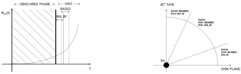
Figure 8.— Left panel: schematic diagram of a pure “evolutionary” model. The mass of the central black hole starts growing in a heavily obscured phase. When it becomes sufficiently luminous to blow away the surrounding medium, it can then be detected as a BALQSO and then finally as an optical, dust-free quasar. Right panel: schematic representation of a simple “orientation” model for RQs and BALQSOs. The radio phase in both schemes is always considered as a brief period within the optical phase.

Figure 9.— Left panel: fraction of FRII-selected sources among the BI-selected BALQSOs (filled circles) and non-BALQSOs (open triangles); both samples have been divided into two subgroups with radio luminosities below and above $L_{\rm 1.4GHz}=2\times 10^{33}\,{\rm erg\,s^{-1}\,Hz^{-1}}$; we display the median luminosity of each subsample. Right panel: absorption index for non-FRII radio sources (open circles) and radio-BI selected FRII sources (filled circles) as a function of radio power. For the more numerous non-FRIIs, we display the mean BI values and associated uncertainties following Hoaglin et al. (1983; see § 4.3).

Figure 10.— Left panel: radio quasar luminosity functions plotted in units of $L^{3}\Phi(L)$ to enhance the differences between the lines; the long-dashed line is the luminosity function of RQs detected as BI BALQSOs, normalized to be 20% the one of the intrinsic total radio quasar luminosity function, which we have assumed to have a slope of $-3.0$; the dotted line is the fraction of $\sim 59\%$ of radio non-beamed, non-BI BALQSOs, while the dot-dashed line is the fraction of $\sim 21\%$ of beamed sources (see text for details); the solid line is the total apparent luminosity function. Right panel: the solid line is the expected fraction of BALQSOs as a function of radio luminosity derived as the ratio of the dashed and solid lines in the left panel; the open circles show the expected fraction averaged over the same radio luminosity bin as the data; all other symbols and lines are as in the left panel of Figure 1.

Figure 11.— Left panel: the crosses in the upper panel show the mean BALQSO Balnicity Index per bin of radio luminosity, while the full sample is shown with points; the middle panel shows the same for the Absorption Index, while the lower panel shows the maximum velocity measured from the absorption troughs as a function of radio luminosity. Right panel: Absorption Index (upper panel) and maximum velocity (lower panel) for AI but not BI-selected BALSQSOs. We do not find any significant trend with radio luminosity for all plotted quantities.

References

- (1) Anderson, S. F., Weymann, R. J., Foltz, C. B., & Chaffee, F. H. 1987, AJ, 94, 278
- (2) Becker, R. H., White, R. L., & Helfand, D. J. 1995, ApJ, 450, 559
- Becker et al. (2000) Becker, R. H., White, R. L., Gregg, M. D., Brotherton, M. S., Laurent-Muehleisen, S. A., & Arav, N. 2000, ApJ, 538, 72
- (4) Becker, R. H., et al. 2001, AJ, 122, 2850
- (5) Blundell, K. M., & Kunzic, Z. 2007, ApJ, 668, 103
- (6) Brotherton, M. S., et al. 1998, ApJ, 505, 7
- (7) Bridle, A. H., & Perley, R. A. 1984, ARA&A, 22, 319
- (8) Condon, J. J., et al. 1998, AJ, 115, 1693
- (9) Croton, D. J., Springel, V., White, S. D. M., De Lucia, G., Frenk, C. S., Gao, L., Jenkins, A., Kauffmann, G., Navarro, J. F., & Yoshida, N. 2006, MNRAS, 365, 11
- Dai et al. (2008) Dai, X., Shankar, F., & Sivakoff, G. R. 2008, ApJ, 672, 108
- (11) De Zotti, G., Ricci, R., Mesa, D., Silva, L., Mazzotta, P., Toffolatti, L., & Gonz lez-Nuevo, J. 2005, A&A, 431, 893
- (12) Fabian, A. C. 1999, MNRAS, 308, 39
- (13) Foltz, C. B., et al. 1986, ApJ, 307, 504
- (14) Francis, P. J., Hooper, E. J., & Impey, C. D. 1993, AJ, 1 06, 417
- (15) Ganguly, R., Bond, N. A., Charlton, J. C., Eracleous, M., Brandt, W. N., & Churchill, C. W. 2001, ApJ, 553, 101
- (16) Ganguly, R., Brotherton, M. S., Cales, S., Scoggins, B., Shang, Z., & Vestergaard, M. 2007, ApJ, 665, 990
- (17) Ganguly, R., & Brotherton, M. S. 2008, ApJ, 672, 102
- (18) Gehrels, N. 1986, ApJ, 303, 336
- (19) Ghosh, K. K., & Punsly, B. 2007, ApJ, 661, 139
- (20) Granato, G. L., Silva, L., Lapi, A., Shankar, F., De Zotti, G., Danese, L. 2006, MNRAS, 368L, 72
- (21) Gregg, M. D., Becker, R. H., & de Vries, W. 2006, ApJ, 641, 210
- Hewett & Foltz (2003) Hewett, P. C., & Foltz, C. B. 2003, AJ, 125, 1784
- (23) Hoaglin, D. C., Mosteller, F., & Tukey, J. W. 1983, in “Understanding robust and exploratory data anlysis”, Wiley Series in Probability and Mathematical Statistics, New York: Wiley, 1983, edited by Hoaglin, D. C., Mosteller, F., & Tukey, J. W.
- (24) Hopkins, P. F., Hernquist, L., Cox, T. J., Di Matteo, T., Robertson, B., & Springel, V. 2006, ApJS, 163, 1
- (25) Jiang, L., Fan, X., Ivezić, Ž., Richards, G. T.; Schneider, D. P., Strauss, M. A., & Kelly, B. C. 2007, ApJ, 656, 680
- (26) Kawakatu, N., Umemura, M., & Mori, M. 2003, ApJ, 583, 85
- (27) Kellermann, K. I., et al. 1989, AJ, 98, 1195
- (28) Kelly, B. C., Bechtold, J., Trump, J. R., Vestergaard, M., & Siemiginowska, A. 2008, ApJ, accepted, arXiv:08012383
- (29) King, A. 2003, ApJ, 596, L27
- (30) Knigge, C., Scaringi, S., Goad, M. R., & Cottis, C. E. 2008, MNRAS, in press, arXiv:0802.3697
- (31) Lapi, A., Shankar, F., Mao, J., Granato, G. L., Silva, L., De Zotti, G., & Danese, L. 2006, ApJ, 650, 42
- (32) Maddox, N., Hewett, P. C., Warren, S. J., & Croom, S. M. 2008, MNRAS, in press, arXiv:0802.3650
- Matthews & Sandage (1963) Matthews, T. A., & Sandage, A. R. 1963, ApJ, 138, 30
- (34) Murray, N., Chiang, J., Grossman, S. A., & Voit, G. M. 1995, ApJ, 451, 498
- (35) Padovani, P., Giommi, P., Landt, H., & Perlman, E. S. 2007, ApJ, 662, 182
- (36) Proga, D., Stone, J. M., & Kallman, T. R. 2000, ApJ, 543, 686
- (37) Richards, G. T., et al. 2006, AJ, 131, 2766
- Schmidt (1963) Schmidt, M. 1963, Nature, 197, 1040
- Schneider et al. (2005) Schneider, D. P., et al. 2005, AJ, 130, 367
- (40) Shankar, F., Lapi, A., Salucci, P., De Zotti, G., & Danese, L. 2006, ApJ, 643, 14
- (41) Shankar, F., Weinberg, D. H., & Miralda-Escudé, J. 2008a, ApJ, submitted, arXiv/0710.4488
- (42) Shankar, F., Cavaliere, A., Cirasuolo, M., & Maraschi, L. 2008b, ApJ, 676, 131
- (43) Shen, Y., Greene, J. E., Strauss, M. A., Richards, G. T., & Schneider, D. P. 2008, ApJ, 680, 169
- (44) Sikora, M., Stawarz, Ł., & Lasota, J.-P. 2007, ApJ, 658, 815
- (45) Snellen, I., & Schilizzi, R. 1999, Invited talk at ‘Lifecycles of Radio Galaxies’ workshop, ed J. Biretta et al., New Astronomy Reviews. astro-ph/9911063
- Stocke et al. (1992) Stocke, J. T., Morris, S. L., Weymann, R. J., & Foltz, C. B. 1992, ApJ, 396, 487
- Trump et al. (2006) Trump, J. R., et al. 2006, ApJS, 165, 1
- (48) Ueda, Y., Akiyama, M., Ohta, K., & Miyaji, T. 2003, ApJ, 598, 886 (U03)
- (49) Urry, M., Padovani, P. 1991, ApJ, 371, 60
- (50) Urry, M., Padovani, P. 1995, PASP, 107, 803
- (51) Vanden Berk, D. E., et al. 2005, AJ, 129, 2047
- (52) Vestergaard, M. 2003, ApJ, 599, 116
- (53) Wang, J., Jiang, P., Zhou, H., Wang, T., Dong, X., & Wang, H. 2008, ApJL, accepeted, arXiv:0802.0253
- (54) Weymann, R. J., Williams, R. E., Peterson, B. M., & Turnshek, D. A. 1979, ApJ, 234, 33
- Weymann et al. (1991) Weymann, R. J., Morris, S. L., Foltz, C. B., & Hewett, P. C. 1991, ApJ, 373, 23
- (56) White, R. L., et al. 2007, ApJ, 654, 99
- (57) Zhou, H., et al. 2006, ApJ, 639, 716