A new method for studying the vibration of non-homogeneous membranes

Abstract

We present a method to solve the Helmholtz equation for a non-homogeneous membrane with Dirichlet boundary conditions at the border of arbitrary two-dimensional domains. The method uses a collocation approach based on a set of localized functions, called ”little sinc functions”, which are used to discretize two-dimensional regions. We have performed extensive numerical tests and we have compared the results obtained with the present method with the ones available from the literature. Our results show that the present method is very accurate and that its implementation for general problems is straightforward.

1 Introduction

This paper focuses on the solution of the inhomogeneous Helmholtz equation

$$-\Delta u(x,y)=E\rho(x,y)u(x,y)$$ (1)

over an arbitrary two dimensional membrane $\mathcal{B}$, with Dirichlet boundary conditions at the border, $\partial\mathcal{B}$. $u(x,y)$ is the transverse displacement and $E=\omega^{2}$, $\omega$ being the frequency of vibration of the membrane.

This problem has been considered in the past by several authors, using different techniques: for example, Masad in [1] has studied the vibrations of a rectangular membrane with linearly varying density using a finite difference scheme and an approach based on perturbation theory; the same problem was also considered by Laura and collaborators in [2], using an optimized Galerkin-Kantorovich approach and by Ho and Chen, [3], who have used a hybrid method. Recently Reutskiy has put forward in [4] a new numerical technique to study the vibrations of inhomogeneous membranes, the method of external and internal excitation. Finally, Filipich and Rosales have studied the vibrations of membranes with a discontinous density profile.

In this paper we describe a different approach to this problem and compare its performance with that of the methods mentioned above. Our method is based on a collocation approach (see for example [7]) which uses a particular set of functions, the Little Sinc functions (LSF), introduced in [8, 9], to obtain a discretization of a finite region of the two-dimensional plane. These functions have been used with success in the numerical solution of the Schrödinger equation in one dimension, both for problems restricted to finite intervals and for problems on the real line. In particular it has been observed that exponential convergence to the exact solution can be reached when variational considerations are made (see [8, 9]). In ref.[9], the LSF were used to obtain a new representation for non–local operators on a grid and thus numerically solve the relativistic Schrödinger equation. An alternative representation for the quantum mechanical path integral was also given in terms of the LSF.

Although Ref.[8] contains a detailed discussion of the LSF, I will briefly review here the main properties, which will be useful in the paper. Throughout the paper I will follow the notation of [8].

A Little Sinc Function is obtained as an approximate representation of the Dirac delta function in terms of the wave functions of a particle in a box (being $2L$ the size of the box). Straightforward algebra leads to the expression

$$s_{k}(h,N,x)\equiv\frac{1}{2N}\ \left\{\frac{\sin\left((2N+1)\ \chi_{-}(x)\right)}{\sin\chi_{-}(x)}-\frac{\cos\left((2N+1)\chi_{+}(x)\right)}{\cos\chi_{+}(x)}\right\}\ .$$ (2)

where $\chi_{\pm}(x)\equiv\frac{\pi}{2Nh}(x\pm kh)$. The index $k$ takes the integer values between $-N/2+1$ and $N/2-1$ ($N$ being an even integer). The LSF corresponding to a specific value of $k$ is peaked at $x_{k}=2Lk/N=kh$, $h$ being the grid spacing and $2L$ the total extension of the interval where the function is defined. By direct inspection of eq. (2) it is found that $s_{k}(h,N,x_{j})=\delta_{kj}$, showing that the LSF takes its maximum value at the $k^{th}$ grid point and vanishes on the remaining points of the grid.

It can be easily proved that the different LSF corresponding to the same set are orthogonal [8]:

$$\int_{-L}^{L}s_{k}(h,N,x)s_{j}(h,N,x)dx=h\ \delta_{kj}$$ (3)

and that a function defined on $x\in(-L,L)$ may be approximated as

$$f(x)\approx\sum_{k=-N/2+1}^{N/2-1}f(x_{k})\ s_{k}(h,N,x)\ .$$ (4)

This formula can be applied to obtain a representation of the derivative of a LSF in terms of the set of LSF as:

$$\frac{ds_{k}(h,N,x)}{dx}\approx\sum_{j}\left.\frac{ds_{k}(h,N,x)}{dx}\right|_{x=x_{j}}\ s_{j}(h,N,x)\equiv\sum_{j}c_{kj}^{(1)}\ s_{j}(h,N,x)$$

$$\frac{d^{2}s_{k}(h,N,x)}{dx^{2}}\approx\sum_{j}\left.\frac{d^{2}s_{k}(h,N,x)}{dx^{2}}\right|_{x=x_{j}}\ s_{j}(h,N,x)\equiv\sum_{j}c_{kj}^{(2)}\ s_{j}(h,N,x)\ ,$$

(5)

where the expressions for the coefficients $c_{kj}^{(r)}$ can be found in [8]. Although eq. (4) is approximate and the LSF strictly speaking do not form a basis, the error made with this approximation decreases with $N$ and tends to zero as $N$ tends to infinity, as shown in [8]. For this reason, the effect of this approximation is essentially to replace the continuum of a interval of size $2L$ on the real line with a discrete set of $N-1$ points, $x_{k}$, uniformly spaced on this interval.

Clearly these relations are easily generalized to functions of two or more variables. Since the focus of this paper is on two dimensional membranes, we will briefly discuss how the LSF are used to discretize a region of the plane; the extension to higher dimensional spaces is straightforward. A function of two variables can be approximated in terms of $(N_{x}-1)\times(N_{y}-1)$ functions, corresponding to the direct product of the $N_{x}-1$ and $N_{y}-1$ LSF in the $x$ and $y$ axis: each term in this set corresponds to a specific point on a rectangular grid with spacings $h_{x}$ and $h_{y}$ (in this paper we use a square grid with $N_{x}=N_{y}=N$ and $L_{x}=L_{y}=L$).

Since $(k,k^{\prime})$ identifies a unique point on the grid, one can select this point using a single index

$$K \equiv k^{\prime}+\frac{N}{2}+(N-1)\left(k+\frac{N}{2}-1\right)$$ (6)

which can take the values $1\leq K\leq(N-1)^{2}$. This relation can be inverted to give

$$k = 1-N/2+\left[\frac{K}{N-1+\varepsilon}\right]$$ (7)

$$k^{\prime} = K-N/2-(N-1)\ \left[\frac{K}{N-1+\varepsilon}\right]\ ,$$ (8)

where $\left[a\right]$ is the integer part of a real number $a$ and $\varepsilon\rightarrow 0$.

To illustrate the collocation procedure we can consider the Schrödinger equation in two dimensions:

$$\hat{H}\psi_{n}(x,y)\equiv\left[-\Delta+V(x,y)\right]\psi_{n}(x,y)=E_{n}\psi_{n}(x,y)$$ (9)

using the convention of assuming a particle of mass $m=1/2$ and setting $\hbar=1$. The Helmholtz equation, which describes the vibration of a membrane, is a special case of (9), corresponding to having $V(x,y)=0$ inside the region $\mathcal{B}$ where the membrane lies and $V(x,y)=\infty$ on the border $\partial\mathcal{B}$ and outside the membrane.

The discretization of eq. (9) proceeds in a simple way using the properties discussed in eqs. (4) and (5):

$$H_{kk^{\prime},jj^{\prime}}=-\left[c^{(2)}_{kj}\delta_{k^{\prime}j^{\prime}}+\delta_{kj}c^{(2)}_{k^{\prime}j^{\prime}}\right]+\delta_{kj}\delta_{k^{\prime}j^{\prime}}V(x_{k},y_{k^{\prime}})$$ (10)

where $(k,j,k^{\prime},j^{\prime})=-N/2+1,\dots,N/2-1$. Notice that the potential part of the Hamiltonian is obtained by simply ”collocating” the potential $V(x,y)$ on the grid, an operation with a limited computational price. The result shown in (10) corresponds to the matrix element of the Hamiltonian operator $\hat{H}$ between two grid points, $(k,k^{\prime})$ and $(j,j^{\prime})$, which can be selected using two integer values $K$ and $J$, as shown in (6).

Following this procedure the solution of the Schrödinger (Helmholtz) equation on the uniform grid generated by the LSF corresponds to the diagonalization of a $(N-1)^{2}\times(N-1)^{2}$ square matrix, whose elements are given by eq. (10).

2 Applications

In this Section we apply our method to study the vibration of different non-homogeneous membranes. Our examples are a rectangular membrane with a linear and oscillatory density, a rectangular membrane with a piecewise constant density, a circular membrane with density $\rho(x,y)=1+\sqrt{x^{2}+y^{2}}$ and a square membrane with a variable density which fluctuates randomly around a constant value. All the numerical calculations have been performed using Mathematica 6.

2.1 A rectangular membrane with linearly varying density

Our first example is taken from [1] and later studied by different authors [2, 3, 4]; these authors have considered the Helmholtz equation over a rectangle of sides $a$ and $b$, and with a density

$$\rho(x,y)=1+\alpha\left(\frac{x}{a}+\frac{1}{2}\right)\ .$$ (11)

Notice that the factor $1/2$ appearing in the expression above derives from our convention of centering the rectangle in the origin, whereas the authors of [1, 2] consider the regions $x\in(0,a)$ and $y\in(0,b)$.

The Helmholtz equation for an inhomogeneous membrane is

$$-\Delta u(x,y)=\omega^{2}\rho(x,y)u(x,y)$$ (12)

where $u(x,y)$ is the transverse displacement and $\omega$ is the frequency of vibration.

As explained in [10], the collocation of the inhomogeneous Helmholtz equation is straightforward, and in fact it does not require the calculation of any integral. The basic step is to rewrite eq. (12) into the equivalent form

$$-\frac{1}{\rho(x,y)}\ \Delta u(x,y)=\omega^{2}u(x,y)\ .$$ (13)

The operator $\hat{O}\equiv-\frac{1}{\rho(x,y)}\ \Delta$ is easily collocated on the uniform grid generated by the LSF, and a matrix representation is obtained. To see how this is achieved we can limit ourselves to a one dimensional operator and make it act over a single LSF:

$$-\frac{1}{\rho(x)}\frac{d^{2}}{dx^{2}}s_{k}(h,N,x) = -\sum_{jl}\frac{1}{\rho(x_{j})}c^{(2)}_{kl}s_{j}(h,N,x)s_{l}(h,N,x)$$ (14)

$$\approx -\sum_{j}\frac{1}{\rho(x_{j})}c^{(2)}_{kj}s_{j}(h,N,x)\ .$$

The matrix representation of this operator over the grid can now be read explicitly from the expression above. It is important to notice that in general the matrix representation of $\hat{O}$ will not be symmetric, unless the membrane is homogeneous. From a computational point of view the diagonalization of symmetric matrices is typically faster than for non-symmetric matrices of equal dimension.

$n$	$N=10$	$N=12$	$N=10$	$N=12$
1	4.335384404	4.335384227	3.610497303	3.610490268
2	6.853837244	6.853836545	5.670792660	5.670765953
3	6.856020159	6.856019330	5.755204660	5.755169941
4	8.672635329	8.672633652	7.290804774	7.290733907
5	9.690424142	9.690422167	7.942675413	7.942603436
6	9.696016734	9.696013642	8.146392098	8.146261520
7	11.05545104	11.05544646	9.299769374	9.299574120
8	11.05628129	11.05627781	9.305141208	9.304993459
9	12.63048727	12.63048290	10.24733083	10.24717742
10	12.64211438	12.64210427	10.62452059	10.62409026

Table 1: Results for the first $10$ frequencies for $b/a=1$ and $\alpha=0.1$ (second and third columns) and to $\alpha=1$ (fourth and fifth columns).

In Table 1 we display the first $10$ frequencies of the square membrane ($b/a=1$) for $\alpha=0.1$ (second and third columns) and for $\alpha=1$ (fourth and fifth columns). The number of collocation points is determined by the parameter $N$ which is fixed to $10$ (second and fourth columns) and to $12$ (third and fifth columns). The comparison of the results corresponding to different $N$ gives us an information over the precision of the results: looking at the Table we see that typically the results agree at least in the first $5$ digits, although we are working with a rather sparse grid. Also it should be remarked that the method is providing a whole set of eigenvalues and eigenvectors, $(N-1)^{2}$ to be exact, whereas in other approaches each mode is studied separately.

To allow a comparison with the results of ref. [1, 2, 3, 4] a calculation of the fundamental frequency of the rectangular membrane for different sizes of the membrane and different density profile is reported in Table 2. The numerical results have been obtained working with $N=12$. These results can be compared with those of Table 1 and 2 of ref. [1], of Table 1 of ref. [2], of Table 1 of ref. [3] and of Table 10 of ref. [4] (in the last two references only the case $\alpha=0.1$ is studied). Comparing our results with those of Masad we have been able to confirm the observation of Laura et al., that the frequencies calculated by Masad for $\alpha=1$ and $b/a=0.6,0.4,0.2$ are incorrect. Actually, the results reported by Masad in these cases are just the second frequency (for $b/a=0.6,0.4$) and the fourth frequency (for $b/a=0.2$) of the corresponding rectangular membrane, which the author failed to identify as such. This observation illustrates the advantage of working with a method which provides a tower of frequencies at the same time.

Another great advantage of our method is the great rate of convergence which is typically observed as the number of grid points is increased. In the cases studied in ref. [10] where the boundary conditions are enforced exactly (a circle and a circular waveguide) we observed that the leading non-constant behaviour of the eigenvalues for $N\gg 1$ was $1/N^{4}$. This analysis in now repeated here for the case of $\alpha=1$ and $b/a=0.2$: the points in Fig.1 correspond to the square of the fundamental frequency calculated using different grid sizes. The curves which decay with $N$ correspond to fitting the numerical points with $f_{r}(N)=c_{0}+c_{1}/N^{r}$ with $r=3,4,5$ respectively. The horizontal line is the limit value of $f_{4}(N)$ for $N\rightarrow\infty$, which corresponds to $\omega=12.548431091$ (notice that the result obtained for $N=12$ agrees in its first five digit with this result, whereas the analogous result of ref. [2] agrees only in three digits). The reader will certainly notice that $f_{4}(N)$ fits excellently the sets, thus confirming the observations made in ref. [10]. A further important observation concerns the monotonic behaviour of the points in the figure: as observed already in ref. [10] this method typically provides monotonic sequences of approximations which approach the exact value from above.

In Fig. 2 we have plotted the first $200$ frequencies of a square membrane with $\alpha=0,0.1,1$ (going from top to bottom), using a grid with $N=26$.

2.2 A rectangular membrane with oscillating density

As a second example, we consider a rectangular membrane with density $\rho(x)=1+0.1\sin\pi(x+1/2)$. This problem has been studied in ref. [3, 4]. In Table 3 we compare our results (LSF) with the results of ref. [3], for different sizes of the membrane. Our results, obtained with a grid corresponding to $N=20$, agree with those of ref. [3]. In Table 4 we compare the results for the first $10$ frequency of the square membrane with this density with those reported in ref. [4]. Although our first $7$ results agree with those of ref. [4], we have noticed that the remaining results do not agree. By looking at the table the reader will notice that the disagreement is caused by the fact that ref. [4] has missed a frequency (such an error cannot take place with our method, since the diagonalization of the Hamiltonian matrix automatically provides the lowest part of the spectrum).

$b/a$	$\alpha=0.1$	$\alpha=1$
1	4.335384227	3.610490268
0.8	4.907186348	4.08151588
0.6	5.957896353	4.942230449
0.4	8.252203964	6.797302677
0.2	15.61334941	12.54867967

Table 2: Results for the fundamental frequency of a rectangular membrane with density $\rho(x)=1+\alpha(x+1/2)$ for $\alpha=0.1$ and $\alpha=1$, using $N=12$.

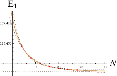
Figure 1: Square of the fundamental frequency of the rectangular membrane for $b/a=0.2$ and $\alpha=1$ as a function of $N$. The dashed, solid and dotted lines correspond to fitting the numerical points with $f_{r}(N)=c_{0}+c_{1}/N^{r}$ with $r=3,4,5$ respectively. The horizontal line is the limit value of $f_{4}(N)$ for $N\rightarrow\infty$, corresponding to $E_{1}=\omega_{1}^{2}=157.4631229$.

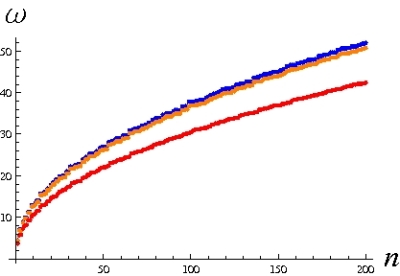
Figure 2: First $200$ frequencies of a square membrane with density $\rho(x)=1+\alpha(x+1/2)$ for $\alpha=0,0.1,1$ (from top to bottom) obtained using $N=26$.

$b/a$	LSF	Ref. [3]
1	4.265402726	4.26541
0.8	4.828066678	4.82806
0.6	5.862077020	5.86207
0.4	8.120442809	8.12044
0.2	15.37382214	15.37381

Table 3: Results for the fundamental frequency of the rectangular membrane with density $\rho(x)=1+\alpha\sin\pi(x+1/2)$ for $\alpha=0.1$, using the LSF with $N=20$ (second column). The third column are the results of Ref.[3].

$n$	LSF	Ref. [4]
1	4.265402726	4.265404
2	6.743887484	6.743888
3	6.797319723	6.797326
4	8.597648785	8.597662
5	9.536589305	9.536574
6	9.624841722	9.624849
7	10.95914134	10.95915
8	10.97412691	12.43285
9	12.43293737	12.55436
10	12.55438511	12.91349
11	12.91343471	$-$

Table 4: First $11$ frequencies of a square membrane with density $\rho(x)=1+0.1\sin\pi(x+1/2)$ using the LSF with $N=20$ (second column). The third column are the results of Ref.[4].

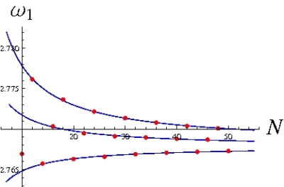
Figure 3: Fundamental frequency of the rectangular membrane with discontinous density. The solid lines are the fits $f(N)=c_{0}+c_{1}/N$ over the three different monotonous sequences of numerical approximations.

2.3 A rectangular membrane with discontinous density

Our next example is taken from ref. [5, 6]: it is a rectangular membrane of sizes $a=1$ and $b=1.8$. The membrane is divided into two regions by the line 

$$y+b/2=0.3(x+a/2)+0.7\ .$$ (15)

The upper region has a density which is twice as big as the density of the lower region. The collocation procedure is the same as in the previous example. In Fig. 3 we have plotted the fundamental frequency of the membrane calculated with different grid sizes, i.e. different $N$. In this case we clearly observe an oscillation of the numerical value: as discussed in ref. [10] this behaviour is typical when the grid does not cross the boundary. Although in the present case the Dirichlet boundary conditions are enforced exactly on the border of the rectangle, the region of discontinuity is not sampled optimally by the grid, which causes the oscillation. Nonetheless, we may observe that the set of numerical values can be divided into three distinct and equally spaced sets, each of which can be fitted quite well with a behaviour $f(N)=c_{0}+c_{1}/N$ (the solid curves in the plot). Going from top to bottom, the curves correspond to the fits:

$$f(N) = 2.76810+0.0975751/N$$ (16)

$$f(N) = 2.76778+0.0395891/N$$ (17)

$$f(N) = 2.76785-0.0304169/N\ .$$ (18)

$n$	$N=34$	$N=40$	$N=46$
1	2.768965729	2.768808666	2.768693679
2	3.967450487	3.967209040	3.966996848
3	4.845749110	4.845534206	4.845424548
4	5.006258593	5.006199469	5.006157369
5	5.844875008	5.844420528	5.844031012
6	6.308222252	6.307796274	6.307464549
7	6.926024314	6.925679216	6.925339604
8	7.006779901	7.006553463	7.006421938
9	7.632533775	7.632317904	7.632118114
10	7.711258827	7.711116778	7.711041692

Table 5: First $10$ frequencies of a rectangular membrane with discontinous density for different grid sizes.

2.4 A circular membrane with density $\rho(x,y)=1+\sqrt{x^{2}+y^{2}}$

Another interesting example is taken from ref. [4], where an inhomogeneous circular membrane with density $\rho(x,y)=1+\sqrt{x^{2}+y^{2}}$ is considered. Table 8 of ref.[4] contains the first $5$ eigenvalues. We have applied our method to this problem, using grids of different sizes, with $N$ going from $10$ to $30$. Studying the $N$ dependence of the eigenvalues, we have seen that these decrease monotonically and that the leading non-constant dependence on $N$ for $N\rightarrow\infty$ is $N^{-3}$ (see Fig.5). In Table 6 we report the first $10$ frequencies of a circular membrane with density $\rho(x,y)=1+\sqrt{x^{2}+y^{2}}$ for different grid sizes ($N=26,28,30$). Notice that the results already agree in their first $4$ digits. A more precise result is then obtained by performing an extrapolation of the numerical results for grids going from $N=12$ to $N=30$. Notice the good agreement with the results of [4] (although we believe that our results are more precise), and that, as expected, some frequencies are degenerate (the degeneracy of the frequencies is not discussed in [4]).

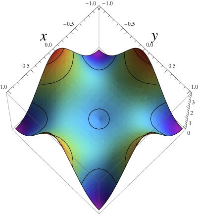
Figure 4: Density of the square inhomogeneous membrane obtained by conformal mapping of the circular homogeneous membrane with density $\rho(x,y)=1+\sqrt{x^{2}+y^{2}}$. The solid lines mark the level $1$,$2$ and $3$.

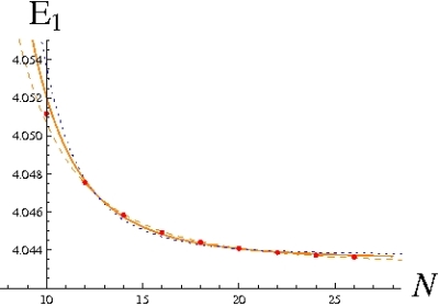
Figure 5: Square of the fundamental frequency of the circular membrane with density $\rho(x,y)=1+\sqrt{x^{2}+y^{2}}$ as a function of $N$. The dashed, solid and dotted lines correspond to fitting the numerical points with $f_{r}(N)=c_{0}+c_{1}/N^{r}$ with $r=3,4,5$ respectively.

$n$	$N=26$	$N=28$	$N=30$	extrapolated	Ref.[4]
1	2.010879124	2.010861686	2.010848852	2.010797145	2.00987
2	3.067875783	3.067856983	3.067843839	3.067802071	3.06760
3	3.067875783	3.067856983	3.067843839	3.067802071	-
4	4.022444836	4.022423309	4.022408260	4.022360463	4.02232
5	4.022616933	4.022550844	4.022504777	4.022359634	-
6	4.555479648	4.555348923	4.555254320	4.554900658	4.55457
7	4.928682458	4.928599914	4.928542452	4.928361919	4.92830
8	4.928682458	4.928599914	4.928542452	4.928361919	-
9	5.699612500	5.699483990	5.699394977	5.699117837	-
10	5.699612500	5.699483990	5.699394977	5.699117837	-

Table 6: First $10$ frequencies of a circular membrane with density $\rho(x,y)=1+\sqrt{x^{2}+y^{2}}$ for different grid sizes. The fourth column reports the frequencies obtained by extrapolating the numerical results for grids going from $N=12$ to $N=30$. The last column reports the results of ref. [4].

2.5 A square membrane with a random density

Our last example is a square membrane with a variable density which fluctuates randomly around the value $\rho_{0}=1$. We have generated random values for the density on a uniform square grid with $81$ points (corresponding to $N_{0}=10$ in our notation); at these points the value of the density has been chosen according to the formula:

$$\rho(x_{k},y_{j})=\rho_{0}+\delta\rho\ q_{kj}$$ (19)

where $\rho_{0}=1$ and $\delta\rho=1/2$. $q_{kj}$ is a random number distributed uniformly between $-1/2$ and $1/2$. The density over all the square has then been obtained interpolating with the LSF:

$$\rho(x,y)=\mathcal{C}\sum_{kj}\rho(x_{k},y_{j})\ s_{k}(h,N_{0},x)s_{j}(h,N_{0},y)\ ,$$ (20)

where $N_{0}=10$, as previously mentioned. $\mathcal{C}$ is a normalization constant which constrains the total mass of the membrane to be equal to the mass carried by the homogeneous membrane with density $\rho_{0}$.

In the left panel of Fig.6 we plot the density of the membrane, while in the right plot we plot the fundamental mode. We have performed our calculation using a grid with $N=40$ (i.e. with a total of $1521$ modes): upon diagonalization of the matrix obtained using the collocation procedure we have obtained numerical estimates for the lowest part of the spectrum of the random membrane. These results may be compared with those of the homogeneous square membrane and with the asymptotic behavior predicted by Weyl’s law [11]:

$$E_{n}^{Weyl}=\frac{4\pi n}{A}+\frac{L}{A}\sqrt{\frac{4\pi n}{A}}\ ,$$ (21)

$A$ being the area and $L$ the perimeter of the membrane. In Fig. 7 we plot the quantity $\Delta_{n}=E_{n}-E_{n}^{Weyl}$ for the homogeneous square membrane (squares) and the square membrane with randomly oscillating density (circles). We have limited the plot to the first $200$ modes. Notice that in both cases $\Delta$ oscillates around $0$, although the oscillation are smaller for the random membrane.

We have also fitted the first $400$ modes with the functional form given by Weyl’s law obtaining

$$E_{n}\approx 3.14546n+3.45835\sqrt{n}$$ (22)

for the homogeneous membrane and

$$E_{n}\approx 3.14445n+3.44674\sqrt{n}$$ (23)

for the random membrane. These values should be compared with the one given by eq. (21):

$$E_{n}\approx 3.14159n+3.54491\sqrt{n}\ .$$ (24)

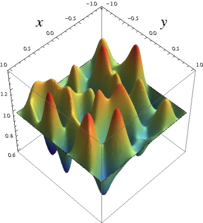
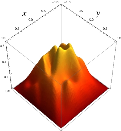
Figure 6: Left Panel:Density of the square membrane with random density (Set 1). Right Panel: Fundamental mode of the square membrane with random density (using Set 1). We have used the LSF on a grid with $N=40$.

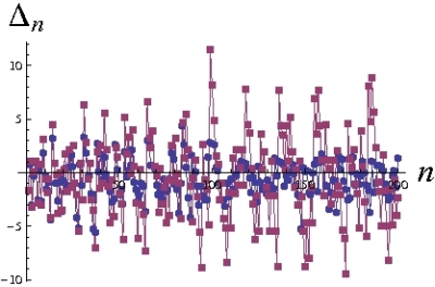
Figure 7: $\Delta_{n}=E_{n}-E_{n}^{Weyl}$ for the homogeneous square membrane (squares) and the square membrane with randomly oscillating density (circles).

3 Conclusions

In this paper we have introduced a new method to solve the Helmholtz equation for non-homogeneous membranes. This method uses the Little Sinc Functions introduced in refs. [8, 9] to obtain a representation of the Helmholtz equation on an uniform grid. The problem thus reduces to diagonalizing a $(N-1)^{2}\times(N-1)^{2}$ square matrix, $N-1$ being the number of collocation points in each direction. We have tested the method on several examples taken from the literature. The application of the method is straightforward and it provides quite accurate results even for grids with moderate values of $N$. The readers interested to looking to more examples of application of this method should check the site

http://fejer.ucol.mx/paolo/drum

where images of modes of vibration of membranes of different shapes can be found.

References

- [1] J.A.Masad, Free vibrations of non-homogeneous rectangular membrane, Journal of Sound and Vibration 195, 674-678 (1996)
- [2] P.A.A.Laura, R.E.Rossi and R.H.Gutierrez, The fundamental frequency of non-homogeneous rectangular membranes, Journal of Sound and Vibration 204, 373-376 (1997)
- [3] S.H.Ho and C.K.Chen, Free vibration analysis of non-homogeneous rectangular membranes using a hybrid method, Journal of Sound and Vibration 233, 547-555 (2000)
- [4] S.Yu. Reutskiy, The methods of external and internal excitation for problems of free vibrations of non-homogeneous membranes, Engineering Analysis with Boundary Elements 31, 906-918 (2007)
- [5] S.W.Kang and J.M.Lee, Free vibration analysis of composite rectangular membranes with an oblique interface, Journal of Sound and Vibration 251, 505-517 (2002)
- [6] C.P.Filipich and M.B.Rosales, Vibration of non-homogeneous rectangular membranes with arbitrary interfaces, Journal of Sound and Vibration 305, 582-595 (2007)
- [7] P. Amore, A variational sinc collocation method for strong-coupling problems, Journal of Physics A 39, L349-L355 (2006)
- [8] P.Amore, M.Cervantes and F.M.Fernández, Variational collocation on finite intervals, J.Phys.A 40, 13047-13062 (2007)
- [9] P.Amore, Alternative representation of nonlocal operators and path integrals, Phys.Rev.A 75, 032111 (2007)
- [10] P. Amore, Solving the Helmholtz equation for membranes of arbitrary shape, sent to Journal of Physics A (2008)
- [11] J.R.Kuttler and V.G.Sigillito, Eigenvalues of the Laplacian in two dimensions, Siam Review 26, 163-193 (1984)