Complex dynamics of a Holling-type IV predator-prey model

Abstract

In this paper, we focus on a spatial Holling-type IV predator-prey model which contains some important factors, such as diffusion, noise (random fluctuations) and external periodic forcing. By a brief stability and bifurcation analysis, we arrive at the Hopf and Turing bifurcation surface and derive the symbolic conditions for Hopf and Turing bifurcation in the spatial domain. Based on the stability and bifurcation analysis, we obtain spiral pattern formation via numerical simulation. Additionally, we study the model with colored noise and external periodic forcing. From the numerical results, we know that noise or external periodic forcing can induce instability and enhance the oscillation of the species, and resonant response. Our results show that modeling by reaction-diffusion equations is an appropriate tool for investigating fundamental mechanisms of complex spatiotemporal dynamics.

I Introduction

Predation, a complex natural phenomena, exists widely in the world, e.g., the sea, the plain, the forest, the desert and so on Cantrell2003 . To model this phenomenon, predator-prey model has been suggested for a long time since the pioneer work of Lotka and Volterra Kendall . The predator-prey model is a kind of “pursuit and evasion” system in which the prey try to evade the predator and the predator try to catch the prey if they interact Murray2003 . Pursuit means the predator try to shorten the spatial distance between the predator and the prey, while evasion means the prey try to widen this spatial distance. In fact, the predator-prey model is a mathematical method to approximate some part of our real world. And the dynamic behavior of the predator-prey model has long been and will continue to be one of the dominant themes in both ecology and mathematical ecology due to its universal existence and importance Berryman ; kuang98global .

Generally, a classical predator-prey model can be written as the form Arditi ; David2002 :

$$\begin{array}[]{l}\frac{dN}{dt}=Nf(N)-mPg(N,P),\qquad\frac{dP}{dt}=P[cmg(N,P)-d],\end{array}$$ (2)

where $N$ and $P$ stand for prey and predator quantity, respectively, $f(N)$ the per capita rate of increase of the prey in absence of predation, $d$ the food-independent death rate of predator, $g(N,P)$ the functional response, the prey consumption rate by an average single predator, which obviously increases with the prey consumption rate and can be influenced by the predator density, and which refers to the change in the density of prey attached per unit time per predator as the prey density changes, $mg(N,P)$ the amount of prey consumed per predator per unit time, and $cmg(N,P)$ the predator production per capita with predation.

In population dynamics, a functional response $g(N,P)$ describes the relationship between the predator and their prey, and the predator-prey model is always named after the corresponding functional response for its key position Ruan ; Abrams ; Arditi ; David2002 . In the history of population ecology, both ecologists and mathematicians have a great interest in the Holling-type predator-prey models Pang ; Jicai2004 ; Ko ; Weipeng ; Gakkhar ; Yuming2004 ; Abrams ; Estep ; Skalski ; Teemu2004 ; Malchow2004 ; Murray2003 ; HUAIPING2002 ; ZhangChen , including Holling type I-III, originally due to Holling Hollinga ; Hollingb , and Holling type IV, suggested by Andrews Andrews . The Holling-type functional responses are so-called “prey-dependent” type Abrams , for $g(N,P)$ in Eq.(2) is a function only related to prey $N$. The classical expression of Holling-type II functional response is $g(N,P)=\frac{mN}{1+b{N}}$, and $g(N,P)=\frac{mN^{2}}{1+a{N}^{2}}$ is called Holling-type III. The Holling-type IV functional response is written as follows:

$$g(N,P)=\frac{mN}{1+bN+a{N}^{2}}.$$ (3)

Fuction (3) is called Monod-Haldane-type functional response too Karen . In addition, when $b=0$, a simplified form $g(N,P)=\frac{mN}{1+a{N}^{2}}$ is proposed by Sokol and Howell Sokolhowell , and some scholars also called it as Holling-type-IV Karen ; Ruan . In this paper, we focus on the Holling-type IV functional response which takes the form (3), and the corresponding predator-prey model which takes the form:

$$\begin{array}[]{l}\frac{dN}{dt}=rN\left(1-{\frac{N}{K}}\right)-{\frac{mNP}{1+bN+a{N}^{2}}},\qquad\frac{dP}{dt}=P\left(-q+{\frac{cmN}{1+bN+a{N}^{2}}}\right),\end{array}$$ (5)

where $r>0$ stands for maximum per capita growth rate of the prey, $m>0$ the capture rate, $c>0$ the conversion rate of prey captured by predator, $q>0$ the food-independent death rate of predator and $K>0$ the carrying capacity, $a>0$ the so-called half-saturation constant, $b>-2\sqrt{a}$ such that the denominator of above system does not vanish for non-negative $N$.

On the other hand, the real world we lived in is a spatial world, and spatial patterns are ubiquitous in nature, which modify the temporal dynamics and stability properties of population density on range of spatial scales, whose effects must be incorporated in temporal ecological models that do not represent space explicitly Claudia . And the spatial component of ecological interactions has been identified as an important factor in how ecological communities are shaped. Empirical evidence suggests that the spatial scale and structure of the environment can influence population interactions and the composition of communities  Cantrell2003 .

Reaction-diffusion model is a typical spatial extended model. It involves not only time but also space and consists of several species which react with each other and diffuse within the spatial domain. It also involves a pair of partial differential equations, and represents the time course of reacting and diffusing process. In the spatial extended predator-prey model, the interaction between the predator and the prey is the reaction item, and the diffusion item comes into being for the predator’s “pursuit” and the prey’s “evasion”. Diffusion is a spatial process, and the whole model describes the evolution of the predator and the prey going with time.

Decades after Turing Turing1952 demonstrated that spatial patterns could arise from the interaction of reactions or growth processes and diffusion, reaction-diffusion models have been studied in ecology to describe the population dynamics of predator-prey model for a long time since Segel and Jackson applied Turing’s idea Segel1972 . Since then, a new field of ecology, pattern formation, came into being. The problem of pattern and scale is the central problem in ecology, unifying population biology and ecosystem science, and marrying basic and applied ecology Levin1992 . And the study of spatial patterns in the distribution of organisms is a central issue in ecology, geology, chemistry, physics and so on Hawick2006 ; Martin2006 ; Cantrell2003 ; RevModPhys.65.851 ; Garvie ; Gierer1972 ; Griffith ; J.Garcia-Ojalvo ; Estep ; Klausmeier06111999 ; Teemu2004 ; Karen ; Maini2002 ; Maini2006 ; Maionchi ; Malchow2004 ; medvinsky:311 ; Murray2003 ; Koichiro ; Wang2007 ; Zhou ; LiZzh2005 ; yang:7259 ; PhysRevLett.88.208303 ; YangLF2004 ; Katsuragi ; Riaz2005 ; Riaz2006 . Theoretical work has shown that spatial and temporal pattern formation can play a very important role in ecological and evolutionary systems. Patterns can affect, for example, stability of ecosystems, the coexistence of species, invasion of mutants and chaos. Moreover, the patterns themselves may interact, leading to selection on the level of patterns, interlocking ecoevolutionary time scales, evolutionary stagnation and diversity.

Based on the above discussions, the spatial extended Holling-type IV predator-prey model with reaction diffusion takes the form:

$$\begin{array}[]{l}\frac{\partial N}{\partial t}=rN\left(1-{\frac{N}{K}}\right)-{\frac{mNP}{1+bN+a{N}^{2}}}+d_{1}\nabla^{2}N,\qquad\frac{\partial P}{\partial t}=P\left(-q+{\frac{cmN}{1+bN+a{N}^{2}}}\right)+d_{2}\nabla^{2}P,\end{array}$$ (7)

where $d_{1}$ and $d_{2}$ are the diffusion coefficients respectively, $\nabla^{2}=\frac{\partial}{\partial x^{2}}+\frac{\partial}{\partial y^{2}}$ the usual Laplacian operator in two-dimensional space, and other parameters are the same definition as those in model (5).

Easy to know that, when a spatial extended predator-prey model is considered, the evolution of the model is decided by two sorts of sources (internal source and external source) which act together. The internal source is the dynamics of the individuals of the model, and the external source is the variability of environment. Some of the variability is periodic, such as temperature, water, food supply of the prey and mating habits. It is necessary and important to consider models with periodic ecological parameters or perturbations which might be quite naturally exposed Cushing . These periodic factors are regarded as the external periodic forcing in the predator-prey systems. The external forcing can affect the population of the predator and prey, respectively, which would go extinct in a deterministic environment. And some of the variability is irregular, such as the the seasonal changes of the weather, food supply of the prey, mating habits, and the affects of this variability are called “noise”. Ecological population dynamics are inevitably “noisy” Kendall . In the predator-prey systems, the random fluctuations are also undeniably arising from either environmental variability or internal species. To quantify the relationship between fluctuations and species’ concentration with spatial degrees of freedom, the consideration of these fluctuations supposes to deal with noisy quantities whose variance might at time be a sizable fraction of their mean levels. For example, the birth and death processes of individuals are intrinsically stochastic fluctuations which becomes especially pronounced when the number of individuals is small Malchow2004 . Moreover, there are many other stochastically factors causing predator-prey population to change, such as effects of spatial structure of the habitat on the predator-prey ecosystem. The interaction between the predator and prey, which are far from being uniformly distributed, also introduce randomness. And these processes can be regarded as parameter fluctuates irregularly with spaces and time.

The induced effects of the external forcing and noise in population dynamics, such as pattern formation, stochastic resonance, delayed extinction, enhanced stability, quasi periodic oscillations and so on, have been investigated with an increasing interest in the past decades YangLF2004 ; J.Garcia-Ojalvo ; Jose1998 ; Spagnolo ; Zhou ; Sifenni ; Liuqx ; Mankin2006 ; Malchow2004 ; Riaz2005 . And noise cannot systematically be neglected in models of population dynamics Jose1998 . Zhou and Kurths Zhou concluded these periodic variabilities as external forcing, and investigated the interplay among noise, excitability, mixing and external forcing in excitable media advected by a chaotic flow, in a two-dimensional FitzHugh-Nagumo model described by a set of reaction-advection-diffusion equations. And Si et al Sifenni studied the propagation of traveling waves in sub-excitable systems driven, and Liu et al Liuqx considered a spatial extended phytoplankton-zooplankton system with additive noise and periodic forcing. Following these models they considered, the Holling-type IV predator-prey model with external periodic forcing and colored noise is as follows:

$$\begin{array}[]{l}\frac{\partial N}{\partial t}=rN\left(1-{\frac{N}{K}}\right)-{\frac{mNP}{1+bN+a{N}^{2}}}+A\sin{(\omega t)}+d_{1}\nabla^{2}N,\\[4.0pt] \frac{\partial P}{\partial t}=P\left(-q+{\frac{cmN}{1+bN+a{N}^{2}}}\right)+\eta(\textbf{\emph{r}},t)+d_{2}\nabla^{2}P,\end{array}$$ (10)

where $A\sin(\omega t)$ denotes the periodic forcing with amplitude $A$ and angular frequency $\omega$. The colored noise term $\eta(\mathbf{r},t)\,\,\,\,(\,\mathbf{r}=(x,y)\,)$ is introduced additively in space and time, referring to the fluctuations in the predator increase rate, which partially results from the environmental factors such as epidemics, weather and nature disasters, and it is the Ornstein-Uhlenbech process that obeys the following linear stochastic partial differential equation

$$\frac{\partial\eta(\mathbf{r},t)}{\partial t}=-\frac{1}{\tau}\eta(\mathbf{r},t)+\frac{1}{\tau}\xi(\mathbf{r},t),$$ (11)

where $\xi(\mathbf{r},t)$ is a Gaussian white noise or the so called Markovian random telegraph process in both space and time with zero mean and correlation:

$$\langle\xi(\mathbf{r},t)\rangle=0,\quad\langle\xi(\mathbf{r},t)\xi(\mathbf{r}^{\prime},t^{\prime})\rangle=2\varepsilon\delta(\mathbf{r}-\mathbf{r}^{\prime})\delta(t-t^{\prime}),$$

where $\langle\cdot\rangle$ denotes mean value with respect to the noise $\xi(\mathbf{r},t)$, and $\delta$ the Dirac delta-function, $\delta(\mathbf{r}-\mathbf{r}^{\prime})$ the spatial correlation function of the Gaussian white noise $\xi(\mathbf{r},t)$ .

Integrating equation (11) with respect to time $t$, we get

$$\eta(\mathbf{r},t)=\eta(\mathbf{r},0)e^{-\frac{t}{\tau}}+\frac{1}{\tau}e^{-\frac{t}{\tau}}\int_{0}^{t}e^{\frac{s}{\tau}}\xi(\mathbf{r},s)ds.$$

The mean value of the colored noise is

$$\langle\eta(\mathbf{r},t)\rangle=\langle\eta(\mathbf{r},0)\rangle e^{-\frac{t}{\tau}}+\frac{1}{\tau}e^{-\frac{t}{\tau}}\int_{0}^{t}e^{\frac{s}{\tau}}\langle\xi(\mathbf{r},s)\rangle ds=\langle\eta(\mathbf{r},0)\rangle e^{-\frac{t}{\tau}},$$

and the correlation function of the colored noise is given by

$$\langle\eta(\mathbf{r},t)\eta(\mathbf{r}^{\prime},t^{\prime})\rangle = \langle\eta(\mathbf{r},0)\rangle\langle\eta(\mathbf{r}^{\prime},0)\rangle e^{-\frac{t+t^{\prime}}{\tau}}+\frac{1}{\tau^{2}}e^{-\frac{t+t^{\prime}}{\tau}}\int_{0}^{t}\int_{0}^{t^{\prime}}e^{\frac{s+s^{\prime}}{\tau}}\langle\xi(\mathbf{r},s)\xi(\mathbf{r}^{\prime},s^{\prime})\rangle dsds^{\prime}$$ (12)

$$= \langle\eta(\mathbf{r},0)\rangle\langle\eta(\mathbf{r}^{\prime},0)\rangle e^{-\frac{t+t^{\prime}}{\tau}}+\frac{\varepsilon}{\tau^{2}}e^{-\frac{t+t^{\prime}}{\tau}}\delta(\mathbf{r}-\mathbf{r}^{\prime})\int_{0}^{t}\int_{0}^{t^{\prime}}e^{\frac{s+s^{\prime}}{\tau}}\delta(t-t^{\prime})dsds^{\prime}$$ (13)

$$= \langle\eta(\mathbf{r},0)\rangle\langle\eta(\mathbf{r}^{\prime},0)\rangle e^{-\frac{t+t^{\prime}}{\tau}}+\frac{\varepsilon}{\tau}\delta(\mathbf{r}-\mathbf{r}^{\prime})(e^{-\frac{t+t^{\prime}}{\tau}}-2e^{-\frac{t}{\tau}}+e^{-\frac{t-t^{\prime}}{\tau}}).$$ (14)

Let $t\rightarrow+\infty$, then

$$\langle\eta(\mathbf{r},t)\eta(\mathbf{r}^{\prime},t^{\prime})\rangle\rightarrow\frac{\varepsilon}{\tau}e^{-\frac{t-t^{\prime}}{\tau}}\delta(\mathbf{r}-\mathbf{r}^{\prime}).$$

The colored noise $\eta(\mathbf{r},t)$ generated in this way represents a simple spatiotemporal structured noise that can be used in real mimic situations, which is temporally correlated and white in space, and satisfies

$$\langle\eta(\mathbf{r},t)\eta(\mathbf{r}^{\prime},t^{\prime})\rangle=\frac{\varepsilon}{\tau}e^{-\frac{|t-t^{\prime}|}{\tau}}\delta(\mathbf{r}-\mathbf{r}^{\prime}),$$

where the temporal memory of the stochastic process controlled by $\tau$ and $\varepsilon$ is the intensity of noise. In this paper, we set $\tau=1$.

Based on these discussion above, in this paper, we mainly focus on the spatiotemporal dynamics of model (7) and (10). And the organization is as follows: In section 2, we employ the method of stability analysis to derive the symbolic conditions for Hopf and Turing bifurcation in the spatial domain. In section 3, we give the complex dynamics of model (7) and (10), involving pattern formation, phase portraits, time series plots and resonant response and so on, via numerical simulation. Then, in the last section, we give some discussions and remarks.

II Hopf and Turing bifurcation

The non-spatial model (5) has at least two equilibria (steady states) which correspond to spatially homogeneous equilibria of the model (7) and (10), in the positive quadrant: $(0,0)$ (total extinct) is a saddle; $(K,0)$ (extinct of the predator, or prey-only) is a attracting node if $q>{\frac{cmK}{1+Kb+a{K}^{2}}}$, a saddle if $q<{\frac{cmK}{1+Kb+a{K}^{2}}}$ or a saddle-node if $q={\frac{cmK}{1+Kb+a{K}^{2}}}$. When

$$\begin{array}[]{l}(a,b,c,m,q,r,K)\in E_{1},\,\,\text{here,}\,\,E_{1}=\{(a,b,c,m,q,r,K)|\,mc>qb,{q}^{2}a<(mc-qb)^{2},\\ \qquad\sqrt{(mc-qb)^{2}-4\,{q}^{2}a}>{\frac{-{m}^{2}{c}^{2}+2\,qbmc+qaKmc-{q}^{2}aKb+2\,{q}^{2}a-{q}^{2}{b}^{2}}{-mc+qb+qaK}}>0,{\frac{b}{a}}-\,{\frac{mc}{qa}}+\,K<0\},\end{array}$$

there exists unique stationary coexistent state $({N_{1}}^{*},{P_{1}}^{*})$, where

$$\begin{array}[]{l}{N_{1}}^{*}={\frac{1}{2}}\,{\frac{-qb+mc-A}{qa}},\qquad{P_{1}}^{*}={\frac{cr\left((-mc\,+bq+qaK\,){N_{1}}^{*}+q\right)}{a{q}^{2}K}}.\end{array}$$

On the other hand, when

$$\begin{array}[]{l}(a,b,c,m,q,r,K)\in E_{2},\,\,\text{here,}\,\,E_{2}=\{(a,b,c,m,q,r,K)|\,mc>qb,{q}^{2}a<(mc-qb)^{2},\\ \qquad\sqrt{(mc-qb)^{2}-4\,{q}^{2}a}>-{\frac{-{m}^{2}{c}^{2}+2\,qbmc+qaKmc-{q}^{2}aKb+2\,{q}^{2}a-{q}^{2}{b}^{2}}{-mc+qb+qaK}}>0,{\frac{b}{a}}-\,{\frac{mc}{qa}}+\,K>0\},\end{array}$$

there exists another unique stationary coexistent state $({N_{2}}^{*},{P_{2}}^{*})$ implying:

$$\begin{array}[]{l}{N_{2}}^{*}={\frac{1}{2}}\,{\frac{-qb+mc+A}{qa}},\qquad{P_{2}}^{*}={\frac{cr\left((-mc\,+bq+qaK\,){N_{2}}^{*}+q\right)}{a{q}^{2}K}}.\end{array}$$

It is worth mentioning that equilibria $(N_{1}^{*},P_{1}^{*})$ and $(N_{2}^{*},P_{2}^{*})$ cannot coexist. In this paper, we mainly focus on the dynamics of $(N_{1}^{*},P_{1}^{*})$ and rewrite it as $(N^{*},P^{*})$. The dynamic behavior of $(N_{2}^{*},P_{2}^{*})$ is similar to those of $(N_{1}^{*},P_{1}^{*})$.

To perform a linear stability analysis, we linearize model (5) around the stationary state $(N^{*},P^{*})$ for small space- and time-dependent fluctuations and expand them in Fourier space

$$N(\mathbf{r},t)\sim N^{*}e^{\lambda t}e^{i\vec{k}\cdot\mathbf{r}},\quad P(\mathbf{r},t)\sim P^{*}e^{\lambda t}e^{i\vec{k}\cdot\mathbf{r}},\quad\mathbf{r}=(x,y),\quad\vec{k}=(k_{x},k_{y}).$$

where $\lambda$ is the eigenvalue of the Jacobian matrix of model (5).

Hopf bifurcation is an instability induced by the transformation of the stability of a focus. Mathematically speaking, Hopf bifurcation occurs when $\text{Im}(\lambda)\neq 0,\quad\text{Re}(\lambda)=0\,\,\,\text{at}\,\,\,k=0$, where $\text{Im}(\lambda)$ is the imaginary part, $\text{Re}(\lambda)$ the real part and $k$ the wave number. So we get the Hopf bifurcation surface

$$H=\{(a,b,c,m,q,r,K)|\,\,\text{det}(J_{0})>0,\text{trace}(J_{0})=0\},$$ (15)

where

$$\begin{array}[]{l}\text{det}(J_{0})=-\left(r-2\,{\frac{rN^{*}}{K}}\right)q+\frac{mqP^{*}+cm\left(r-2\,{\frac{rN^{*}}{K}}\right)N^{*}}{\left(1+bN^{*}+a{N^{*}}^{2}\right)}-{\frac{mqN^{*}P^{*}\left(b+2\,aN^{*}\right)}{\left(1+bN^{*}+a{N^{*}}^{2}\right)^{2}}},\\[8.0pt] \text{trace}(J_{0})=r-2\,{\frac{rN^{*}}{K}}-q+{\frac{m\left(-P^{*}+cN^{*}+a{N^{*}}^{2}P^{*}+bc{N^{*}}^{2}+c{N^{*}}^{3}a\right)}{\left(1+bN^{*}+a{N^{*}}^{2}\right)^{2}}},\end{array}$$

the frequency of periodic oscillations in time $\omega_{H}$ satisfies $\omega_{H}=\text{Im}(\lambda)=\sqrt{\text{det}(J_{0})}$, and the corresponding wavelength $\lambda_{H}$ satisfies $\lambda_{H}=\frac{2\pi}{\omega_{H}}=\frac{2\pi}{\sqrt{\text{det}(J_{0})}}\,.$ Especially, we take $K$ as the bifurcation parameter, and can get the critical value of Hopf bifurcation from Eq. (15):

$$\begin{array}[]{l}K_{H}=(-(a{q}^{2}(5\,mc-3\,qb)-(3\,mc-qb)(mc-qb)^{2})\sqrt{(mc-qb)^{2}-4\,{q}^{2}a}\\[8.0pt] -4\,{q}^{4}{a}^{2}+{q}^{2}(mc-qb)(11\,mc-5\,qb)a-(3\,mc-qb)(mc-qb)^{3})/(-aq(((2\,mc-qb)\\[8.0pt] (mc-qb)-2\,{q}^{2}a)\sqrt{(mc-qb)^{2}-4\,{q}^{2}a}-2a{q}^{2}(3\,mc-2\,qb)+(2\,mc-qb)(mc-qb)^{2})).\end{array}$$ (16)

Turing instability is induced only by “pursuit and evasion” if the predator can catch the prey by pursuit. We call the critical state of Turing instability as Turing bifurcation. Turing bifurcation occurs when $\text{Im}(\lambda)=0,\,\,\text{Re}(\lambda)=0\,\,\text{at}\,\,k=k_{T}\neq 0,$ and the wavenumber $k_{T}$ satisfies $k_{T}^{2}=\sqrt{\frac{\text{det}(J_{0})}{d_{1}d_{2}}}$. In addition, at the Turing threshold, the spatial symmetry of the system is broken and the patterns are stationary in time and oscillatory in space with the wavelength $\lambda_{T}=\frac{2\pi}{k_{T}}$. And the Turing bifurcation surface implies:

$$T=\{(a,b,c,m,q,r,d_{1},d_{2},K)|\quad\text{det}(J_{k})=0,\text{trace}(J_{k})=0\},$$ (17)

where

$$\begin{array}[]{l}\text{det}(J_{k})=-\left(r-2\,{\frac{rN^{*}}{K}}-d_{{1}}{k}^{2}\right)\left(q+d_{{2}}{k}^{2}\right)\frac{\left(\left(q+d_{{2}}{k}^{2}\right)mP^{*}+\left(r-2\,{\frac{rN^{*}}{K}}-d_{{1}}{k}^{2}\right)cmN^{*}\right)}{1+bN^{*}+a{N^{*}}^{2}}\\[8.0pt] \qquad\qquad\,\,\,-{\frac{m\left(b+2\,aN^{*}\right)\left(q+d_{{2}}{k}^{2}\right)N^{*}P^{*}}{(1+bN^{*}+a{N^{*}}^{2})^{2}}},\\[8.0pt] \text{trace}(J_{k})=r-2\,{\frac{rN^{*}}{K}}-q-\left(d_{{1}}+d_{{2}}\right){k}^{2}+{\frac{m\left(-P^{*}+cN^{*}+a{N^{*}}^{2}P^{*}+bc{N^{*}}^{2}+c{N^{*}}^{3}a\right)}{\left(1+bN^{*}+a{N^{*}}^{2}\right)^{2}}},\end{array}$$

the critical value of Turing bifurcation can be obtained from Eq. (17) as follows:

$$K_{{T}}={\frac{F_{{1}}}{F_{{2}}}},$$ (18)

where

$${\begin{array}[]{l}F_{{1}}=r((4\,{q}^{2}a(2\,mc-qb)-(3\,mc-qb)(mc-qb)^{2})\sqrt{(mc-qb)^{2}-4\,{q}^{2}a}+((mc-qb)^{2}-4\,{q}^{2}a)\\[4.0pt] \qquad\qquad\cdot((3\,mc-qb)(mc-qb)-2\,{q}^{2}a))((3\,mc-qb)(mc-qb)-4\,{q}^{2}a\\[4.0pt] \qquad\qquad-(3\,mc+qb)\sqrt{(mc-qb)^{2}-4\,{q}^{2}a}\,\,)d_{{2}},\\[8.0pt] \end{array}}$$

$${\begin{array}[]{l}F_{{2}}=qa(2\,mc((mc-qb)\sqrt{(mc-qb)^{2}-4\,{q}^{2}a}+4\,{q}^{2}a-(mc-qb)^{2})B+((3\,mc-qb)d_{{2}}\\[4.0pt] \qquad\qquad\cdot(2\,{m}^{2}{c}^{2}-3\,qbmc+{q}^{2}{b}^{2}-4\,{q}^{2}a)r+2\,qd_{{1}}mc(mc-qb)^{2})({(mc-qb)^{2}-4\,{q}^{2}a})\\[4.0pt] \qquad\qquad+(-2\,d_{{2}}((3\,mc-qb)(2\,mc-qb)(mc-qb)^{2}-2\,{q}^{2}a(-4\,{q}^{2}a+3\,{q}^{2}{b}^{2}-12\,qbmc\\[4.0pt] \qquad\qquad+11\,{m}^{2}{c}^{2}))r-4\,qcm(mc-qb)d_{{1}}((mc-qb)^{2}-4\,{q}^{2}a))\sqrt{(mc-qb)^{2}-4\,{q}^{2}a}\\[4.0pt] \qquad\qquad+({q}^{2}{b}^{2}-2\,qbmc+{m}^{2}{c}^{2}-4\,{q}^{2}a)((2\,mc-qb)d_{{2}}(3\,{m}^{2}{c}^{2}-4\,qbmc+{q}^{2}{b}^{2}-4\,{q}^{2}a)r\\[4.0pt] \qquad\qquad+2\,mcqd_{{1}}((mc-qb)^{2}-4\,{q}^{2}a))),\\[8.0pt] B=(-2\,d_{{1}}q(((d_{{1}}b{q}^{2}-qd_{{1}}mc-qrbd_{{2}}+2\,rmcd_{{2}})(4\,{q}^{2}a-(mc-qb)^{2})-rmcd_{{2}}(mc-qb)^{2})\\[4.0pt] \qquad\qquad\cdot\sqrt{(mc-qb)^{2}-4\,{q}^{2}a}+(8\,{q}^{4}d_{{2}}r-8\,{q}^{5}d_{{1}}){a}^{2}+4\,(mc-qb)a{q}^{2}rmcd_{{2}}+(3\,rmcd_{{2}}\\[4.0pt] \qquad\qquad-qd_{{1}}mc+d_{{1}}b{q}^{2}-qrbd_{{2}})((mc-qb)^{3}-6\,(mc-qb)a{q}^{2})))^{\frac{1}{2}}.\end{array}}$$

Linear stability analysis yields the bifurcation diagram with $r=1$, $a=0.125$, $b=1$, $c=0.7$, $m=0.625$, $q=0.18$ and $d_{2}=0.2$ shown in Figure 1(A). In this case, parameters $(a,b,c,m,q,r,K)\in E_{1}$, and $(N^{*},P^{*})$ is the unique stationary coexistent state. From Figure 1(a), one can see that the Hopf bifurcation line and the Turing bifurcation curve separate the parametric space into three distinct domains. In domain I, located below all two bifurcation lines, the steady state is the only stable solution of the model. Domain II is the region of pure Hopf instability. When the parameters correspond to domain III, located above all two bifurcation lines, both Hopf and Turing instability occur. Figure 1(b) displays the dispersion relations showing unstable Hopf mode, transition of Turing mode from stable to unstable for model (7), e.g., as $d_{1}$ decreased. Figure 1(c) illustrates the relation between the real and the imaginary parts of the eigenvalue $\lambda$ with $K=2.8>K_{H}=2.279$, located in domain II, one can see that when $k=0$, $\text{Re}(\lambda(k))>0$ and $\text{Im}(\lambda(k))\neq 0$. Figure 1(d) displays the case of the critical value of Turing bifurcation $K=K_{T}=3.499$, in this case, $\text{Re}(\lambda(k))=0$ and $\text{Im}(\lambda(k))=0$ at $k=k_{T}=2.080$. When $K=4.0$, located in domain III, figure 1(e) indicates that at $k=0$, $\text{Re}(\lambda(k))>0$, $\text{Im}(\lambda(k))\neq 0$.

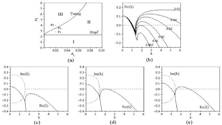
Figure 1: (a) $K-d_{1}$ Bifurcation diagram for model (7) with $r=1$, $a=0.125$, $b=1$, $c=0.7$, $m=0.625$, $q=0.18$ and $d_{2}=0.2$. Hopf and Turing bifurcation lines separate the parameter space into three domains. $P_{1}(0.02,2.8)$, $P_{2}(0.02,3.499)$, $P_{3}(0.02,4.0)$ are the different selections corresponding to (c), (d), (e), respectively. (b) Dispersion relations showing unstable Hopf mode, transition of Turing mode from stable to unstable for the system model (7) as $d_{1}$ decreased. The other parameters in (c)–(e) are: $d_{1}=0.02$, the bifurcation parameter $K$ equals: (c) $2.8>K_{H}=2.279$; (d) $3.499=K_{T}$; (e) $4.0>K_{T}>K_{H}$. The real parts $\text{Re}(\lambda)$ and the imaginary parts $\text{Im}(\lambda)$ are shown by solid curves and dashed curves, respectively.

III Spatiotemporal dynamics of the models

In this section, we perform extensive numerical simulations of the spatially extended model (7) and (10) in two-dimensional spaces, and the qualitative results are shown here. All our numerical simulations employ the Zero-flux Neumann boundary conditions with a system size of $200\times 200$ space units. The parameters are $r=1$, $a=0.125$, $b=1$, $c=0.7$, $m=0.625$, $q=0.18$, $d_{1}=0.02$, $d_{2}=0.2$ and $K=2.8$ or $K=4.0$, which satisfy $(a,b,c,m,q,r,K)\in E$. Model (7) and (10) are integrated initially in two-dimensional space from the homogeneous steady state, i.e., we start with the unstable uniform solution $(N^{*},P^{*})$ with small random perturbation superimposed, in each, the initial condition is always a small amplitude random perturbation $(\pm 5\times 10^{-4})$, using a finite difference approximation for model (7) or Fourier transform method for model (10) for the spatial derivatives and an explicit Euler method for the time integration with a time stepsize of $\Delta t=1/24$ and space stepsize (lattice constant) $\Delta x=\Delta y=1$. We have taken some snapshots with white (black) corresponding to the high (low) value of prey $N$.

In the numerical simulations, different types of dynamics are observed and we have found that the distributions of the predator and prey are always of the same type. Consequently, we can restrict our analysis of pattern formation to one distribution. In this section, we show the distribution of prey $N$, for instance.

III.1 Pattern formation of model (4)

Figure 2 shows the evolution of the spatial patterns of prey $N$ at $t=0$, 100, 300, 500, 1000, 2000, with random small perturbation of the equilibrium $(N^{*},P^{*})=(0.748,2.132)$ of model (7) with $K=2.8$, located in domain II, more than the Hopf bifurcation threshold $K_{H}=2.279$ and less than the Turing bifurcation threshold $K_{T}=3.499$. In this case, pure Hopf instability occurs. One can see that for model (7), the random initial distribution (c.f., figure 2(a)) leads to the formation of macroscopic spiral patterns (c.f., figures 2(d) to (f)). In other words, in this situation, spatially uniform steady-state predator-prey coexistence is no longer. Small random fluctuations will be strongly amplified by diffusion, leading to nonuniform population distributions. From the analysis in section 2, we find with these parameters in domain II, the spiral pattern arises from Hopf instability. The lower panel in figure 2 shows the corresponding (g) time series and (h) phase portraits. Figure 2(g) illustrates the evolution process of prey $N$, periodic oscillating in time finally, (h) exhibits that a limit cycle arises, which is caused by the Hopf bifurcation.

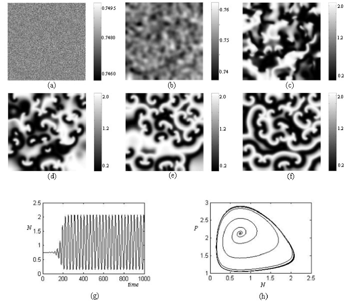
Figure 2: Grey-scaled snapshots of spatiotemporal pattern of the prey $N$ of model (7) with $K=2.8$. (a) $t=0$, (b) $t=100$, (c) $t=300$, (d) $t=500$, (e) $t=1000$, (f) $t=2000$. The lower panels show the corresponding (g) time series plots and (h) phase portraits.

When $K=4.0>K_{T}>K_{H}$, in this case, parameters in domain III (figure 1(A)), both Hopf and Turing instabilities occur. The nontrivial stationary state is $(N^{*},P^{*})=(0.748,2.365)$. As an example, the formation of a regular macroscopic two-dimensional spatial pattern is shown in figure 3. The lower panel in figure 3 shows the corresponding (g) time series plots and (h) phase portraits.

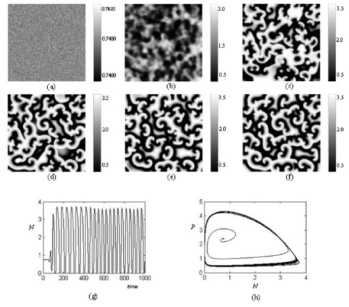
Figure 3: Grey-scaled snapshots of spatiotemporal pattern of the prey $N$ of model (7) with $K=4.0$. (a) $t=0$, (b) $t=100$, (c) $t=300$, (d) $t=500$, (e) $t=1000$, (f) $t=2000$. The lower panels show the corresponding (g) time series plots and (h) phase portraits.

Comparing this situation (figure 3) with the one above (figure 2), easy to see that the pattern formations are all spiral wave. From the analysis in section 2, we know that when $K=2.8$, the wavelength $\lambda=3.100$ while at $K=4.0$, $\lambda=3.021$. And the frequency of periodic oscillations in time is as inverse proportion to wavelength, so we can know that Turing instability has a positive effect on the frequency and negative effect on wavelength. This is the reason why the spiral curves are more dense in figure 3(f) than in figure 2(f). On the other hand, one can see that when $K=4.0$, the time series plots (c.f., figure 3(g)) indicate that when Turing instability occurs, the solution of model (7) is strongly oscillatory in time while with $K=2.8$ (pure Hopf bifurcation emerges) it is periodic (c.f., figure 2(g)). In addition, comparing figure 2(g) with figure 3(g), one can see that Turing instability has a positive effects on the amplitude of prey $N$. And from figure 3(h), one can see that a quasi limit cycle emerges while in figure 2(h), it is a cycle. Although there are some different points between figure 2 and figure 3, but we can know that Turing instability can’t give birth to different type patterns. In our previous work Wang2007 , we find that Turing instability can change pattern type. This may be a very point between the Holling-type IV with Michael-Menton functional response of predator-prey model.

On the other hand, the basic idea of diffusion-driven instability in a reaction-diffusion system can be understood in terms of an activator-inhibitor system or predator-prey model (7). The functioning of this mechanism is based on three points David2002 . First, a random increase of activator species (prey, $N$) should have a positive effect on the creation rate of both activator (prey, $N$) and inhibitor (prey, $P$) species. Second, an increment in inhibitor species should have a negative effect on formation rate of both species. Finally, inhibitor species $P$ must diffuse faster than activator species $N$. Certainly, the reaction-diffusion predator-prey model (7), with Holling-type IV functional response and predators diffusing faster than prey (i.e., $d_{2}>d_{1}$), provides this mechanism. And spirals and curves are the most fascinating clusters to emerge from the predator-prey model. A spiral will form from a wave front when the prey line (which is leading the front) overlaps the pursuing line of predator Hawick2006 . The prey on the extreme end of the line stops moving as there is no predator in the immediate vicinity. However, the prey $N$ and the predator $P$ in the center of the line continue moving forward. This forms a small trail of prey at one (or both) ends of the front. These prey start breeding and the trailing line of prey thickens and attracts the attention of predator at the end of the fox line that turn towards this new source of prey. Thus a spiral forms with predator $P$ on the inside and prey $N$ on the outside. If the original overlap of prey occurs at both ends of the line a double spiral will form. Spirals can also form as a prey blob collapses after the predator eats into it. This is the reason why the pattern formation of model (7) is spiral wave.

III.2 The effect of noise only of model (5)

Now, we turn our focus on the effect of noise on the predator $P$ of stochastic model (10). In this case, $A=0$, i.e., the periodic forcing is not at presence.

Figure 4 shows the dynamics of model (10) with noise on the predator. The first row of figure 4, i.e., (a), $\varepsilon=0.0001$; the second row, (b), $\varepsilon=0.01$; the third row, (c), $\varepsilon=0.05$; and the last row of figure 4, (d), $\varepsilon=0.1$. And the first collum of figure 4, marked as (i), shows the snapshots of spatiotemporal pattern of model (10) at $t=2000$ with different intensity of noise, respectively. In this case, one can see that the pattern formation turns into spatial chaotic from spiral wave with the increase of noise intensity $\varepsilon$. And the second collum of figure 4, marked as (ii), displays the phase portraits of model (10) with different intensity of noise, respectively. We can see that, as noise intensity $\varepsilon$ increasing, the symmetry of the limit cycle is broken and gives rise to chaos. The last collum of figure 4, (iii), illustrates the time-series plots of prey $N$ with different intensity of noise, respectively. One can see that noise breaks the periodic oscillations in time and gives rise to drastically ruleless oscillations in time.

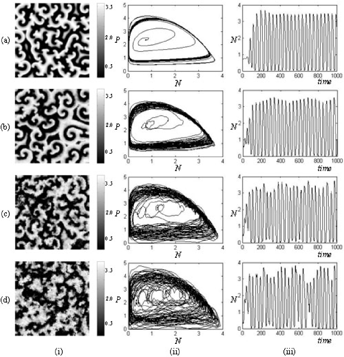
Figure 4: Dynamics of model (7), for the following noise intensity. (a) $\varepsilon=0.0001$; (b)$\varepsilon=0.01$; (c)$\varepsilon=0.05$; (d)$\varepsilon=0.1$. (i) snapshots of pattern formation at time $2000$; (ii) phase portraits; (iii) time-series plots. $A=0$ and the other parameters are the same as those in figure 2.

III.3 The effect of periodic forcing of model (5)

In the previous subsection, we have shown the effect of noise on the predator $P$ of model (10). An interesting question is whether such noise-sustained oscillations can be entrained by a weak external forcing, in this case, $\varepsilon=0$, which is investigated here.

When model (10) is noise free, there is a phenomenon of frequency locking or resonant response Liuqx ; Mankin2006 ; Zhou ; Sifenni . That is, without noise, the spatially homogeneous oscillation does not respond to the external periodic forcing when the amplitude $A$ is below a threshold whose value depends on the external periodic $T_{in}=\frac{2\pi}{\omega}$. Above the threshold, model (10) may produce oscillations about period $T_{out}$ with respect to external period $T_{in}$, which is called frequency locking or resonant response. That is, the model produces one spike within each of the $M=\frac{T_{out}}{T_{in}}$ periods of the external force, called $M:1$ resonant response Zhou ; Sifenni . The phenomenon of coherent resonance is of great importance Mankin2006 . Following Si Sifenni , in the present paper, the output periodic $T_{out}$ is defined as follows: $T_{i}$ is the time interval between the $i$th spike and $(i+1)$th spike. $m$ spikes are taken into account and the average value of them is $T_{out}=\sum\limits_{i=1}^{m}T_{i}/(m-1)$.

As an example, with the amplitude $A=0.001$, figure 5 shows $5:1$ resonant response with $\omega=0.2\pi$ (a) and $\omega=0.02\pi$ (c), respectively. And figure 5(b) and (d) are the phase portraits corresponding to (a) and (c). We can see that when $\omega=0.2\pi$, there exists a periodic orbit, while $\omega=0.02\pi$, a periodic-2 orbit of model (10) emerges. Obviously, different $\omega$ can form the same resonant response, and different phase orbits, i.e., different numerical solution of model (10), may correspond to the same resonant response.

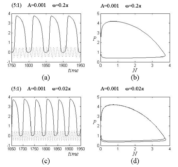
Figure 5: External periodic forcing induced frequency locking of model(7). The solid curve is time series of prey $U$, the dash curve is the corresponding external periodic forcing. Other parameters are the same as those in figure 3.

III.4 The effect of noise and periodic forcing of model (5)

Now, we consider the dynamics about resonant response of model (10) with both noise and periodic forcing. As depicted in figure 6, the prey can generate $5:1$ (a), $4:1$ (c) locked oscillations, depending on the amplitude $A$ and angular frequency $\omega$. Figures 6 (b) and (d) illustrate the spiral pattern at $t=2000$ corresponding to (a) and (c), respectively. For contrast, we change one of the parameters of figure 6(c) $A=0.001$ to $A=0.01$ (e), one can see that the resonant response vanishes, the corresponding spiral pattern (f) is similar to (b). It indicates that the amplitude $A$ is a control factor for pattern formation. In addition, comparing figures 6(b) with (d), one can see that the pattern formations are determined by noise intensity $\varepsilon$, too.

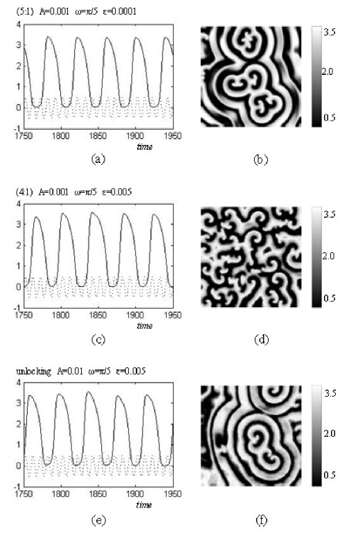
Figure 6: Dynamics of model (10) with both noise and periodic forcing. (b)(d)(f) are snapshots at $t=2000$ corresponding to the left hand side resonant response. The other parameters are the same as those in figure 3.

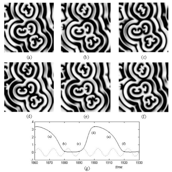
Figure 7: Typical pattern formation of the forced noisy prey in the $5:1$ locking region at $A=0.001$ and $\varepsilon=0.0001$ corresponding to figure 6(a). The lower panel shows the time series of the prey $N$ (the solid curve) and the corresponding external periodic forcing (the dash curve) corresponding to the snapshots of the patterns. The grey scale, from black to white, is in $[0,3.5]$ for all the snapshots.

In Figure 7, we have shown a typical pattern formation process in the $5:1$ frequency locking regime with $A=0.001$ and $\omega=0.2\pi$. From $t=1870$ (a) to $t=1920$ (f), the pattern formation of prey $N$ is spiral wave and some small excitations already develop. One can see that, during the second periodic of the forcing, the prey is almost fully synchronized and relaxes slowly back to the state at moment (f). Obviously, the external periodic forcing at moment (e) repeats that at moment (a). However, the prey $N$ does not exactly repeat due to a small fluctuation of the phase difference.

IV Conclusions and remarks

In this paper, we present spatial Holling-type IV predator-prey model containing some important factors, such as noise (random fluctuations), the external periodic forcing and diffusion processes. And the numerical simulations were consistent with the predictions drawn from the bifurcation analysis, that is, Hopf bifurcation and Turing bifurcation.

If the parameter $K$, the carrying capacity, located in the domain II of figure 1(a), the Hopf instability occurs, the destruction of the pattern begins from the prey $N$, while it begins from the predator $P$ if $K$ located in the domain III, both Hopf and Turing instabilities occur.

Furthermore, we demonstrate that noise and the external periodic forcing play a key role in the predator-prey model (10) with the numerical simulations. We provoke qualitative transformations of the response of the model by changing noise intensity, and noise can enhance the oscillation of the species density, and format large clusters in the space. The periodic oscillations appear when the spatial noise and external periodic forcing are turned on. It has also been realized that model (10) is very sensitive to external periodic forcing through the natural annual variation of prey growth. In conclusion, we have shown that the cooperation between noise and external periodic forcing inherent to the deterministic dynamics of periodically driven models gives rise to the appearance of resonant response.

Significantly, model (10) exhibits oscillations when both noise and external forcing are present. This means that the predator population may be partly due to the external forcing and stochastic factors instead of deterministic factors. Therefore, the model for spatially extended systems composed by two species could be useful to explain spatiotemporal behavior of populations whose dynamics is strongly affected by noise and the environmental physical variables, and the results of this paper are an important step toward providing the theoretical biology community with simple practical numerical methods, for investigating the key dynamics of realistic predator-prey models.

- (1) Abrams P. A. and Ginzburg L. R., 2000. The nature of predation: prey dependent, ratio dependent or neither? Trends Ecol. Evol. 15, 337-341.
- (2) Andrews J. F., 1968. A mathematical model for the continuous culture of microorganisms utilizing inhibitory substrates, Biot. Bioe. 10, 707-723.
- (3) Alonso D., Bartumeus F. and Catalan J., 2002. Mutual interference between predators can give rise to Turing spatial patterns, Ecology 83, 28-34.
- (4) Arditi R. and Ginzburg L. R., 1989. Coupling in predator-prey dynamics: ratio-dependence, J. Theo. Biol. 139, 311-326.
- (5) Baurmann M., Gross T. and Feudel U., 2007. Instabilities in spatially extended predator-prey systems: Spatio-temporal patterns in the neighborhood of Turing-Hopf bifurcations, J. Theo. Biol. 245, 220-229.
- (6) Berryman A., 1992. The origins and evolution of predator-prey theory, Ecology 75, 1530-1535.
- (7) Cantrell R., and Cosner C., 2003. Spatial Ecology via Reaction-Diffusion Equations, John Wiley & Sons, Ltd., Chichester, England.
- (8) Chen Y., 2004. Multiple periodic solutions of delayed predator Cprey systems with type IV functional responses, Nonl. Anal.: Real World Appl. 5, 45-53.
- (9) Cross M. C. and Hohenberg P. C., 1993. Pattern formation outside of equilibrium, Rev. Mod. Phys. 65, 851-1112.
- (10) Cushing J., 1977. Periodic time-dependent predator-prey system, SIAM J. Appl. Math 32, 82-95.
- (11) Estep D. and Neckels D., 2007. Fast methods for determining the evolution of uncertain parameters in reaction-diffusion equations, Computer Methods in Applied Mechanics and Engineering 196, 3967-3979.
- (12) Gakkhar S. and Singh B., 2007. The dynamics of a food web consisting of two preys and a harvesting predator, Chaos, Solitons and Fractals 34, 1346-1356.
- (13) Garcia-Ojalvo J. and Schimansky-Geier L., 1999. Noise-induced spiral dynamics in excitable media, Europhys. Lett. 47, 298-303.
- (14) Garvie M., 2007. Finite-difference schemes for reaction-diffusion equations modelling predator-prey interactions in matlab, Bull. Math. Biol. 69, 931-956.
- (15) Gierer A. and Meinhardt H., 1972. A theory of biological pattern formation, Kybernetik 12, 30-39.
- (16) Griffith D. A. and Peres-Neto P. R., 2006. Spatial modeling in ecology: the flexibility of eigenfunction spatial analyses, Ecology 87, 2603-2613.
- (17) Hawick, K., James, H. and Scogings, C., 2006. A zoology of emergent life patterns in a predator-prey simulation model, Technical Note CSTN-015 and in Proc. IASTED International Conference on Modelling, Simulation and Optimization, September 2006, Gabarone, Botswana. 507-115.
- (18) Holling C. S., 1959. The components of predation as revealed by a study of small mammal predation of the european pine sawfly, Cana. Ento. 91, 293-320.
- (19) Holling C. S., 1959. Some characteristics of simple types of predation and parasitism, Cana. Ento. 91, 385-395.
- (20) Huang J. and Xiao D., 2004. Analyses of Bifurcations and Stability in a Predator-prey System with Holling Type-IV Functional Response, Acta Mathematicae Applicatae Sinica, English Series 20, 167-178.
- (21) Katsuragi H., 2006. Diffusion-induced spontaneous pattern formation on gelation surfaces. Europhys. Lett. 73, 793-799.
- (22) Kendall B., 2001. Cycles, chaos, and noise in predator-prey dynamics, Chaos Solitons Fractals 12, 321-332.
- (23) Klausmeier C.A., 1999. Regular and Irregular Patterns in Semiarid Vegetation, Science 284, 1826-1828.
- (24) Ko W. and Ryu K., 2007. Coexistence states of a predator-prey system with non-monotonic functional response, Nonl. Anal.: Real World Appl. 8, 769-786.
- (25) Kuang Y. and Beretta E., 1998. Global qualitative analysis of a ratio-dependent predator-prey system, J. Math. Biol. 36, 389-406.
- (26) Leppänen T., 2004. Coputational studies of pattern formation in Turing systems, PhD-Thesis, Helsinki University of Technology.
- (27) Levin S. A., 1992. The Problem of Pattern and Scale in Ecology, Ecology 73, 1943-1967.
- (28) Liu Q., Li B., Jin Z., 2007. Resonant patterns and frequency-locked induced by additive noise and periodically forced in phytoplankton-zooplankton system, Preprint: arXiv:0705.3724.
- (29) Li Z., Gao M., Hui C., Han X. and Shi H., 2005. Impact of predator pursuit and prey evasion on synchrony and spatial patterns in metapopulation, Ecol. Model. 185, 245-254.
- (30) Madzvamuse A., Thomas R. D. K. , Maini P. K. and Wathen A. J., 2002. A Numerical Approach to the Study of Spatial Pattern Formation in the Ligaments of Arcoid Bivalves, Bull. Math. Biol. 64, 501-530.
- (31) Maini P. K., Baker R. E. and Chuong C., 2006. The Turing model comes of molecular age, Science 314, 1397-1398.
- (32) Maionchi D. O., Reis S. F. and Aguiar M. A. M., 2006. Chaos and pattern formation in a spatial tritrophic food chain, Ecol. Model. 191, 291-303.
- (33) Mankin R., Laas T., Sauga A. and Ainsaar A., 2006. Colored-noise-induced Hopf bifurcations in predator-prey communities, Phys. Rev. E 74, 021101.
- (34) Malchow H., Hilker F. M., Petrovskii S. V., 2004. Noise and productivity dependence of spatiotemporal pattern formation in a prey-predator system, Disc. Cont. Dyna. Syst. B 4, 705-711.
- (35) Medvinsky A. B., Petrovskii S. V., Tikhonova I. A., Malchow H. and Li B.-L., 2002. Spatiotemporal Complexity of Plankton and Fish Dynamics, SIAM Review 44, 311-370.
- (36) Murray J., 2003. Mathematical biology. II. Spatial models and biomedical applications, 3rd edn., Interdisciplinary Applied Mathematics 18, Springer, New York.
- (37) Neuhauser C., 2001. Mathematical Challenges in Spatial Ecology, Notices of the American Mathematical Society 47, 1304-1314.
- (38) Pang P. Y. H. and Wang M. X., 2004. Non-constant positive steady positive steady statesof a predator-prey system with non-monotonic functional responctionlresponse and diffusion, Proc. Lond. Math. Soc. 88, 135-157.
- (39) Page K., Maini P. K. and Monk N. A. M., 2003. Pattern formation in spatially heterogeneous Turing reaction-diffusion models, Phys. D 181, 80-101.
- (40) Riaz S. S., Dutta S., Kar S. and Ray D. S., 2005. Pattern formation induced by additive noise: a moment-based analysis, Eur. Phys. J. B 47, 255-263.
- (41) Riaz S. S., Banarjee S., Kar S. and Ray D. S., 2006. Pattern formation in reaction-diffusion system in crossed electric and magnetic fields, Eur. Phys. J. B 53, 509-515.
- (42) Ruan S. G. and Xiao D. G., 2001. Global Analysis in a Predator-Prey System with Nonmonotonic Functional Response, SIAM J. Appl. Math. 61, 1445-1472.
- (43) Segel L. A. and Jackson J. L., 1972. Dissipative structure: An explanation and an ecological example, J. Theo. Biol. 37, 545-559.
- (44) Si F., Liu Q., Zhang J. and Zhou L., 2008. Propagation of travelling waves in sub-excitable systems driven by noise and periodic forcing, Eur. Phys. J. B 60, 507-513
- (45) Sokol W. and Howell J. A., 1987. Kinetics of phenol oxidation by washed cell, Biot. Bioe. 30, 921-927.
- (46) Spagnolo B., Valenti D. and Fiasconaro A., 2004. Noise in ecosystems: a short review, Math. Bios. Engi. 1, 185-211.
- (47) Skalski G. T. and Gilliam J. F., 2001. Functional responses with predator interference: Viable alternatives to the Holling type II model, Ecology 82, 3083-3092.
- (48) Turing A. M., 1952. The chemical basis of morphogenisis, Phil. Tran. R. Soc. London B 237, 7-72.
- (49) Uriu K. and Iwasa Y., 2007. Turing Pattern Formation with Two Kinds of Cells and a Diffusive Chemical, Bull. Math. Biol. 69, 2515-2536.
- (50) Vilar J. M. G. and Sole R. V., 1998. Effects of Noise in Symmetric Two-Species Competition, Phys. Rev. Lett. 80, 4099-4102.
- (51) Wang W., Liu Q. and Jin Z., 2007. Spatiotemporal complexity of a ratio-dependent predator-prey system, Phys. Rev. E 75, 051913.
- (52) Yang L., Dolnik M., Zhabotinsky A. and Epstein, I., 2002. Pattern formation arising from interactions between turing and wave instabilities, J. Chem. Phys. 117, 7259-7265.
- (53) Yang L., Milos D., Zhabotinsky A. M. and Epstein I. R., 2002. Spatial Resonances and Superposition Patterns in a Reaction-Diffusion Model with Interacting Turing Modes, Phys. Rev. Lett. 88, 208303.
- (54) Yang L., Zhabotinsky A. M. and Epstein I. R., 2004. Stable Squares and Other Oscillatory Turing Patterns in a Reaction-Diffusion Model, Phys. Rev. Lett. 92, 198303.
- (55) Zhang S., Tan D. and Chen L., 2006. Chaos in periodically forced Holling type IV predator Cprey system with impulsive perturbations, Chaos, Soli. Frac. 27, 980-990.
- (56) Zhang W., Zhu D. and Bi P., 2007. Multiple positive periodic solutions of a delayed discrete predator-prey system with type IV functional responses, Appl. Math. Lett. 20, 1031-1038.
- (57) Zhou C., Kurths J., 2005. Noise-sustained and controlled synchronization of stirred excitable media by external forcing, New J. Phys. 7, 18.
- (58) Zhu H., Campbell S. A. and Wolkowicz G., 2002. Bifurcation analysis of a predator-prey system with nonmonotonic functional response, SIAM J. Appl. Math. 63, 636-682.
- (59)