Recovering the topology of the IGM at z$\sim$2

Abstract

We investigate how well the 3D density field of neutral hydrogen in the Intergalactic Medium (IGM) can be reconstructed using the Lyman-$\alpha$ absorptions observed along lines of sight to quasars separated by arcmin distances in projection on the sky. We use cosmological hydrodynamical simulations to compare the topologies of different fields: dark matter, gas and neutral hydrogen optical depth and to investigate how well the topology of the IGM can be recovered from the Wiener interpolation method implemented by Pichon et al. (2001). The global statistical and topological properties of the recovered field are analyzed quantitatively through the power-spectrum, the probability distribution function (PDF), the Euler characteristics, its associated critical point counts and the filling factor of underdense regions. The local geometrical properties of the field are analysed using the local skeleton by defining the concept of inter-skeleton distance.

As a consequence of the nearly lognormal nature of the density distribution at the scales under consideration, the tomography is best carried out on the logarithm of the density rather than the density itself. At scales larger than $\sim 1.4\langle d_{\rm LOS}\rangle$, where $\langle d_{\rm LOS}\rangle$ is the mean separation between lines of sight, the reconstruction accurately recovers the topological features of the large scale density distribution of the gas, in particular the filamentary structures: the inter-skeleton distance between the reconstruction and the exact solution is smaller than $\langle d_{\rm LOS}\rangle$. At scales larger than the intrinsic smoothing length of the inversion procedure, the power spectrum of the recovered Hi density field matches well that of the original one and the low order moments of the PDF are well recovered as well as the shape of the Euler characteristic. The integral errors on the PDF and the critical point counts are indeed small, less than 20% for a mean line of sight separation smaller than $\sim$2.5 arcmin. The small deviations between the reconstruction and the exact solution mainly reflect departures from the log-normal behaviour that are ascribed to highly non-linear objects in overdense regions.

1 Introduction

The structure and composition of the intergalactic medium (IGM) has long been studied using the Ly-$\alpha$ forest in QSO absorption spectra [Rauch 1998]. The progress made in high resolution Echelle-spectrographs has led to a consistent picture in which the absorption features are related to the distribution of neutral hydrogen through the Lyman transition lines of Hi. Hydrogen in the IGM is highly ionized (Gunn & Peterson, 1965). Its photoionization equilibrium in the expanding IGM establishes a tight correlation between neutral and total hydrogen density and numerical simulations have confirmed the existence of this correlation. They have also shown that the gas density traces the fluctuations of the DM density on scales larger than the Jeans length (see for example Cen et al. 1994, Petitjean et al. 1995, Miralda-Escudé et al. 1996, Theuns et al. 1998, Viel, Haehnelt & Springel 2004).

As we will show in the first part of this work, the statistical and topological properties of the IGM and of the dark matter distributions are the same, so that recovering the three-dimensional distribution and inferring the topological properties of the IGM allows us to constrain the properties of the dark matter distribution as well.

Although topological tools have been introduced only relatively recently in cosmological analysis, they have been used extensively to characterize the topology of large scales structures as revealed by the three-dimensional distribution of galaxies in the local universe (see for exemple Gott et al. (1986), Vogeley et al. (1994), Protogeros & Weinberg (1997), Trac et al. (2002), Park et al.(2005) and Sousbie et al. (2006) for the topological analysis of galaxy surveys). The outcome of such an analysis is a quantitative description of the complex appearance of the distribution of the matter in the universe, with its network of clump, voids, filaments and sheet-like structures. The study of the topology using galaxy surveys is attractive because of their large volume and the huge number of objects they contain. However the clustering of highly non linear objects (galaxies, clusters of galaxies or QSOs) is biased compared to the underlying clustering of dark matter fluctuations that we wish to constrain (see Kaiser 1984). This biasing results from a complicated and delicate competition between a variety of processes which are often too complicated to be tractable analytically. Besides, the maximum redshift in surveys is low (in the analysis of the SDSS data made by Park et al. 2005, the maximum redshift is $z=0.1654$), so that this kind of analysis can be done only in the local Universe, where the fluctuations have already entered the highly non-linear regime.

Given the strong correlation existing between dark matter distribution and the low-density intergalactic medium, one could probe the underlying distribution of matter via the signature produced by diffuse hydrogen in quasar spectra, namely absorption features observed in the Ly-$\alpha$ forest. Indeed, absorption spectra provide a picture complementary to those drawn by galaxy surveys to infer the large scale distribution of the matter in the Universe, since the absorption features produced by the IGM in Ly-$\alpha$ forest can be detected also at large redshift and since the IGM probes the low density range, whereas the galaxy distribution does not. Eventually, higher density contrasts can be recovered from the analysis of the Ly-$\alpha$ forest if higher order transitions are included in the analysis; for example, the Ly-$\beta$ transitions should allow us to probe density contrasts up to $\delta\approx 15$.

The flux along a single line-of-sight towards a quasar only provides one dimensional information, which can be used to constrain the fluctuation amplitude and the matter density (Nusser & Haehnelt 1999, Rollinde et al. 2001, Zaroubi et al. 2006). The transverse information, found in pairs of quasars, has been used to study the extension of the absorbing regions (e.g. Petitjean et al. 1998; Crotts & Fang 1998; Young, Impey & Foltz 2001; Aracil et al. 2002) and the geometry of the Universe at $z\sim 2$ (Hui, Stebbins & Burles 1999; McDonald & Miralda-Escudé 1999; Rollinde et al. 2003, Coppolani et al. 2006).

Given a set of lines of sight (LOSs) toward a group of QSOs with small angular separation, inversion methods can be used to recover the three-dimensional distribution of low density gas, as demonstrated in Pichon et al. (2001). They showed that the visual characterization of the density field (with its network of filaments, clumps, voids and pancakes) is correctly reproduced if the mean separation between the LOSs is less than $\langle d_{\rm LOS}\rangle\leq 5$ Mpc.

In this paper we test quantitatively whether such an inversion can recover the global properties of connectivity of the density field, using topological tools such as the Euler characteristic and the probability distribution function.

The paper is organized as follows. In Section 2, the Euler characteristic is defined as an alternate critical points count and implemented for a Gaussian field. The difference between the topological properties of the dark matter, of the gas and of the observed optical depth is then discussed using outputs of a hydrodynamical simulation (Section 3) and relying on different statistical tools. In Section 4, the ability to reconstruct the global topology of the three dimensional distribution from a simple Wiener interpolation of a discrete group of lines of sight is considered. Finally, Section 5 summarizes the results of this paper and discusses some possible improvements of the method as well as observational constrains from future surveys.

2 The Euler characteristic: an alternate critical point count

This paper makes use of various statistical tools, namely the PDF, the Euler characteristic, the skeleton and related estimators such as the first cumulants of the PDF (connected moments), critical point counts and the filling factor, to characterize the topology of the large scale density distribution. These tools will also be used to test the efficiency of reconstructing the density field from a grid of QSO sight-lines and in particular the ability to reproduce the connectivity of the large scale structures.

Following Colombi, Pogosyan & Souradeep (2000, hereafter CPS), this section introduces the Euler characteristic, ${\tilde{\chi}}^{+}$, as an alternate critical point count in an overdense excursion with density contrasts larger than a threshold $\delta_{\rm TH}$. It is shown how the behavior of ${\tilde{\chi}}^{+}$ is related to connectivity in the field. The numerical implementation used to measure it is described and tested on Gaussian random realizations.

2.1 Definition of the Euler characteristic

Let $\delta({\mathbf{x}})$ be a scalar function defined in a 3D volume $V$. Given a threshold value $\delta_{\rm TH}$, consider the excursion set $E^{+}$ formed by the points ${\mathbf{x}}$ with $\delta({\mathbf{x}})\geq\delta_{\rm TH}$, as expressed by the following equation:

$$E^{+}\equiv\{\mathbf{x}|\delta({\mathbf{x}})>\delta_{\rm TH}\}\,.$$ (1)

The analysis of the geometrical properties of points that belong to the excursion set $E^{+}$ as a function of $\delta_{\rm TH}$ gives information about the global topology of the scalar field $\delta({\mathbf{x}})$ and allows for the characterization of large scale structures.

A simple qualitative link can be established between the distribution of critical points (defined by $\nabla\delta=\mathbf{0}$), a on the one hand, and connectivity on the other, which are related to local and global properties of the excursion set respectively. If one considers over-dense regions, connectivity happens along ridges (filaments) passing through saddle points and connecting local maxima. The same reasoning can be applied to under-dense regions where minima are connected through tunnels (pancakes) via another kind of saddle point. This idea is in fact supported on rigorous grounds by Morse theory (see Milnor 1963). The Morse theorem establishes the link between the distribution of critical points and the global connectivity of the excursion set, via the Euler characteristic. This quantity represents the integral of the Gaussian curvature over an iso-density surface that marks the boundary of the excursion set (see for exemple Gott, Melott & Dickinson, 1986). It is usually defined as the following count (see for example Mecke, Buchert & Wagner, 1994, for details):

$${\tilde{\chi}}^{+}={\rm connected\ components}-{\rm tunnels}+{\rm cavities}.$$ (2)

According to Morse theorem, it can also be expressed as a linear combination of the number of critical points of different types that are found in the excursion set as a function of $\delta_{\rm TH}$.

To be more specific, let us consider the critical points of the field. For these points, the Hessian matrix, whose components are given by:

$${\mathcal{H}}_{i,j}=\frac{\partial^{2}\delta}{\partial x_{i}\partial x_{j}}\,,$$ (3)

is calculated and its eigenvalues are estimated. According to the number of negative eigenvalues, $I$, of the Hessian matrix, the local structures of the field can be classified in the following way: a clump, a filament, a pancake and a void corresponding to $I=$3, 2, 1 and 0 respectively. The Morse theorem states that the Euler characteristic can be expressed as a count of the number of critical points belonging to each of these four classes:

$${\tilde{\chi}}^{+}=N_{I=3}-N_{I=2}+N_{I=1}-N_{I=0}\,,$$ (4)

where $N_{I=i}$ is the number of critical points with $i$ negative eigenvalues. With this approach, it is sufficient to determine the number distribution of the four kinds of critical point. However this differential method requires the field under consideration to be sufficiently smooth and non degenerate. To this end, in the subsequent analyses of this paper, the field will be smoothed with a Gaussian window (using standard FFT technique),

$$W(r)=\frac{1}{(2\pi)^{3/2}L_{s}^{3}}\exp\left(-\frac{r^{2}}{2L_{\rm s}^{2}}\right),$$ (5)

of sufficiently large size $L_{s}$ compared to the sampling grid pixel size in order to minimize the impact of numerical artefacts coming from the discretization of the field on a grid (see, e.g., CPS for a thorough analysis of measurement issues). In what follows, the smoothing scale used to measure the Euler characteristic is always larger than $0.01\times N_{\rm pix}$ grid pixels where $N_{\rm pix}=256$ pixels is the box resolution of the simulations. In principle this smoothing scale is large enough to have an unbiased measurement of the Euler characteristic. The prescription of CPS is used to detect and classify critical points. This method involves locally fitting a second order hypersurface on the smoothed density field, while taking into account each point on the grid under consideration and its 26 neighbors.

2.2 Interpretation of the Euler characteristics

Figure 1: Mean Euler characteristics, $\chi^{+}$ (see Eqs. 4 and 6), for a Gaussian random field (GRF, points with small errorbars) as a function of the density threshold, $\delta/\sigma$, compared to the theoretical prediction (Doroshkevich, 1970, smooth curve). The mean is carried over 5 realizations of a GRF whose power spectrum is given by a power-law with spectral index $n=-1$ on a $256^{3}$ grid, while additional smoothing is performed with a Gaussian window of size $5$ pixels.

Figure 2: Evolution of the number of critical points entering the computation of the Euler characteristic for the GRF considered in Fig. 1. The fraction of different types of critical points above the threshold is plotted as a function of $\delta/\sigma$ and each distribution is compared to the analytical prediction. Again, symbols with error bars represent the mean over 5 realizations of the same GRF, while the smooth curves give the analytical prediction (which can be easily derived from Bardeen et al. 1986).

For clarity, let us recall here the interpretation of the shape of the Euler characteristic as a function of density threshold (CPS). Let us first study the simple case of a Gaussian random field (GRF). The analytic predictions for a GRF are given, for example, in Doroshkevich (1970) (see also, Schmalzing & Buchert 1997). In what follows, a slightly different normalization from Eq. (4) is used: the volume independent quantity

$${\chi}^{+}={\tilde{\chi}}^{+}/N_{\rm tot},$$ (6)

where $N_{\rm tot}=\sum_{i}N_{I=i}$ is the total critical point count in the volume considered, in the limit $\delta_{\rm TH}\rightarrow-\infty$.

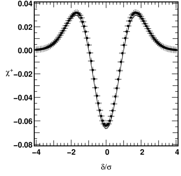
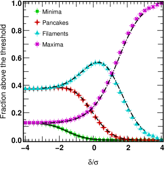
In Figure 1, the numerical estimates of the Euler characteristic are given as a function of the density threshold $\delta_{\rm TH}=\delta/\sigma$ where $\delta=(\rho-\bar{\rho})/\bar{\rho}$ is the density contrast and $\sigma={\rm rms}(\delta)$ from five Gaussian random field (GRF) realizations (points with error bars) whose power spectrum is given by a power-law with spectral index $n=-1$, i.e. $P(k)\propto k^{n}$. The result is compared with the analytic prediction (solid line). The shape of the curve as a function of the density threshold can be understood from Equation (4) and Figure 2 which displays the critical point counts. At very low values of the threshold ($\delta/\sigma\la-4$) the excursion set includes almost all points and, due to the symmetry between high and low-density regions, the number of minima (pancakes) compensates the number of maxima (filaments) so that the Euler characteristic approaches zero. When the value of the threshold is increased, local minima first drop out of $E^{+}$, creating cavities and thus increasing the value of $\chi^{+}$. At $\delta/\sigma\mbox{$\>\stackrel{{\scriptstyle>}}{{{}_{\sim}}}\>$}-2$, pancakes start to drop out too and cavities connect together, thus the value of $\chi^{+}$ decreases, reaching its minimum at $\delta/\sigma\approx 0$. In the range $0\mbox{$\>\stackrel{{\scriptstyle<}}{{{}_{\sim}}}\>$}\delta/\sigma\mbox{$\>\stackrel{{\scriptstyle<}}{{{}_{\sim}}}\>$}2$ filaments also drop out, breaking up the ridges to create isolated clusters, thus increasing $\chi^{+}$ again. Finally in the region $\delta/\sigma\mbox{$\>\stackrel{{\scriptstyle>}}{{{}_{\sim}}}\>$}2$ only clumps are found to lie in the excursion set, but they are progressively lost as the threshold increases, explaining the final decrease of the curve.

This simple analysis shows how the features seen in the Euler characteristic are closely related to the network of filaments and pancakes that connect clumps and voids.

3 From dark matter to optical depth

The Lyman-$\alpha$ absorption lines observed in QSOs spectra and produced by the Hi structures intercepted by the line-of-sight can be used to study the topology of the Universe at high redshift ($z\mbox{$\>\stackrel{{\scriptstyle>}}{{{}_{\sim}}}\>$}1-2$). However, the information derived from observations of QSOs spectra is more directly related to the Hi optical depth, whereas here the aim is to constrain the underlying dark matter density field for which theory makes direct predictions. Hence, one has to rely on simulations in order to calibrate the relation between the density field of the neutral hydrogen and that of the dark matter.

In this section we first present the hydrodynamical simulations used in the present work and we then analyse the shape of the PDF and the Euler characteristic of the three density fields (dark matter, gas and Hi) and of the optical depth field, explaining how these curves are related.

3.1 Numerical simulations

We analyse a cosmological hydrodynamical simulation that evolves both dark matter particles and a gaseous component to study the global topology of the intergalactic medium at redshift $z=2$. The dynamical evolution and the physical properties of the gas and the of the Hi component are calculated taking into account the heating and cooling processes and the effect of the ionizing UV background in a standard way. The corresponding Particle-Mesh (PM) code used to perform the simulation is described in detail in Coppolani et al. (2006).

In this run, the standard $\Lambda$CDM model is assumed with a set of cosmological parameters given by: $\Omega_{\rm m}=0.3$ and $\Omega_{\rm\Lambda}=0.7$, while the assumed baryon density is $\Omega_{\rm b}=0.04$. The Hubble constant is H${}_{0}=70\,{\rm km\,s^{-1}\,Mpc^{-1}}$ and the amplitude of the fluctuations of the matter density field in a sphere of radius $8\ h^{-1}$ Mpc is $\sigma_{8}=1$. While the other cosmological parameters are roughly in agreement with recent observational constraints, the value of $\sigma_{8}$ is somewhat large compared to the value suggested by WMAP (see Spergel et al., 2007). However, this should not have any incidence on the results derived in this paper.

The simulation involved $512^{3}$ dark matter particles in a box with periodic boundary conditions of comoving size $L_{\rm box}=40$ Mpc. The gaseous component was also followed on a $512^{3}$ grid which was used to compute gravitational forces. Although this simulation marginally resolves the Jeans length of the gas, Coppolani et al. (2006) checked with higher resolution runs that numerical convergence was achieved at small scales.

Although $512^{3}$ grid points were available, this resolution was degraded to a $256^{3}$ resolution (using standard donner cell procedure), in order to make the calculations more tractable. Obviously this additional smoothing makes the effects of subclustering within the Jeans length irrelevant. Therefore the gaseous component should be nearly indistinguishable from the dark matter component.

The main limit in these analyses remains the box size, which is still small and only allows for a fair statistical measure at scales $L_{\rm s}$ larger than $L_{\rm max}\sim L_{\rm box}/10$, i.e. 4 Mpc. Indeed finite volume effects are known to become significant for $L_{\rm s}\ga L_{\rm max}$ for standard statistics such as the probability function (see, e.g., Colombi, Bouchet & Schaeffer 1994) and the Euler number (see, e.g., CPS). For the reconstruction, the typical separation $\langle d_{\rm LOS}\rangle$ between lines of sight defines a natural smoothing scale $L_{\rm s}\simeq\langle d_{\rm LOS}\rangle$. Note that, unfortunately, the upper bound of $L_{\rm s}\sim 4$ Mpc corresponds to a lower bound on $\langle d_{\rm LOS}\rangle$ in current state of the art observations [Rollinde et al. 2003], but one can expect to lower this limit in future surveys [Theuns & Srianand 2006]. Hence the following analyses are performed in the range $2\ {\rm Mpc}\leq L_{\rm s}\leq 4$ Mpc.

Figure 3: Probability distribution function of density fields at different smoothing scales (from left to right, top to bottom, no smoothing, $L_{\rm s}$=1.6, $2.2$ and $3.6$ Mpc). The thick solid, thick dashed and thin solid curves correspond to dark matter, gas and Hi (rescaled according to Eq. 7), respectively. The dotted curve is a best fit of a lognormal distribution to the thin solid curve, showing that all these PDFs are reasonably close to lognormal, a property that will be useful for the reconstruction. In the unsmoothed case, the gas and H i PDFs match very well for $1+\delta\mbox{$\>\stackrel{{\scriptstyle<}}{{{}_{\sim}}}\>$}1$ but depart from each other at higher density. The apparent very good match in the unsmoothed case comes from the fact that the un-shocked part of the intergalactic medium totally dominates the part of the PDF which is visible in this panel. The match between Hi and gas PDFs decreases with increasing smoothing scale, due to “mixing effects”, as explained in the main text. Note finally that the dark matter is not displayed in the unsmoothed panel because the result would be contaminated by the cloud-in-cell interpolation used to compute the density on the grid.

Figure 4: Same as in Fig. 3 but for the measured Euler characteristic as a function of density threshold at different smoothing scales. Again, the thick solid, thick dashed and thin solid curves correspond respectively to dark matter, gas and Hi (rescaled according to Eq. 7 with the values $(A,\alpha)$ given in Table 1). While the curves for the dark matter and for the gas superpose exactly at all smoothing scales and all values of the threshold, the Hi, even after the scaling is applied, behaves in a different way in the high density region. As explained in the text, this is a consequence of the presence of shocks and condensed objects, whose effect is a change in connectivity properties.

3.2 PDF and Euler characteristic of physical density fields

It this Section we compare the large-scale distribution and the topological properties of the different density fields (dark matter, total amount of gas and neutral gas) by looking at their probability distribution function (PDF) and their Euler characteristic ($\chi^{+}$). Our knowledge of the physics of the intergalactic medium is used to perform the analysis and to link the distributions of Hi and H. Indeed, the observations give access to the Hi optical depth through absorption spectra. We also consider thermal broadening and redshift distortion effects.

3.2.1 From dark matter to Hi: IGM equation of state

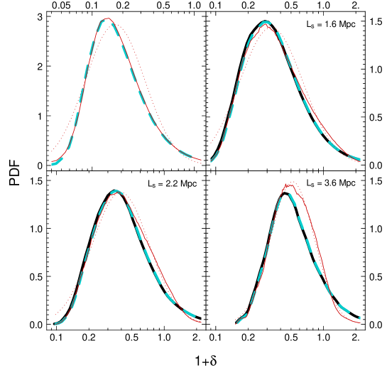
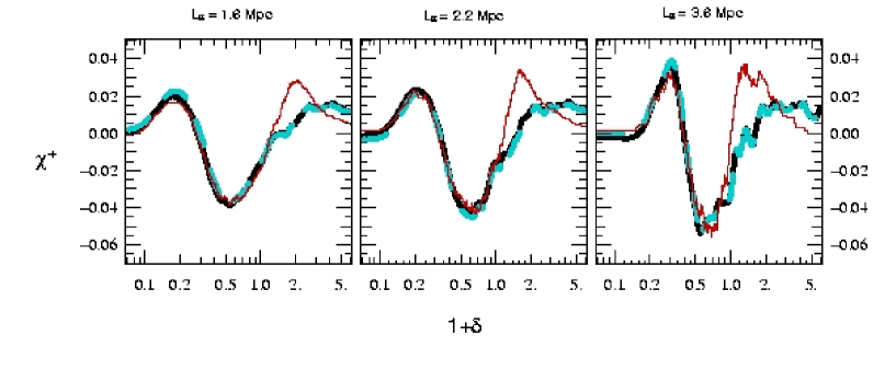
It is well known that on scales larger than the Jeans length the distribution of the gas follows the distribution of dark matter, so that their statistical and topological properties are expected to be the same at these scales. This is checked by comparing the PDF and the Euler characteristic of the two density fields smoothed using different values of $L_{\rm s}$, as shown in Figs. 3 and 4. Note the agreement of the PDFs and of the Euler characteristics of the two fields for all values of the smoothing scale considered, a result which can be expected since the scaling regime probed is largely above the Jeans length of the gas.

(a) Gas density and temperature

(b) Ratio R=${\tilde{\rho}_{\rm HI}}/\rho_{\rm gas}$

Figure 5: Top: Gas density and temperature (in units of $10^{4}$ K) spatial distributions in a one pixel ($\approx 15.6$ kpc) slice. The intensity of the fields is color-coded with the scale given on the right. The panels on the left give the contours corresponding to $\delta=1$ for the density and to $T/10^{4}=2$ for the temperature. Bottom: For the same slice as above we show on the right the spatial distribution of the ratio $R={\tilde{\rho}_{\rm HI}}/\rho_{\rm gas}$ for the unsmoothed field (up) and for the field smoothed with a Gaussian window of size (FWHM) $L_{\rm s}=2.2$ Mpc (down). The color scale is such that darker regions correspond to low values of $R$. On the left the contours correspond to $R=0.7$.

Figure 6: Scatter plots displaying the relation between the gas density and the Hi density at different smoothing scales. The dashed black lines in each panel represent the best fit, following Eq. (7), with the parameters $(A,\alpha)$ given in Table 1. Note that the dispersion increases when the smoothing scales increases, due to the mixing effect discussed in Figure 5.

The comparison of the distribution of the neutral gas (Hi) with that of the total amount of gas and the dark matter calls for a slightly more elaborate approach, given the non-linearity involved in the expression that relates the distribution of the gas to the distribution of Hi. In fact, numerical simulations support the idea that a tight correlation exists between neutral and total hydrogen density (Cen et al. 1994, Miralda-Escudé et al. 1996, Theuns et al. 1998, Viel, Haehnelt & Springel 2004). This correlation is expected to follow a power-law of the form

$$\rho_{\rm gas}\approx A\cdot(\rho_{H{\sc i}})^{\alpha}\,.$$ (7)

We thus introduce here a new density field $\tilde{\rho}_{\rm H{\sc i}}$ defined as the right-hand-side of Equation (7), so that $\tilde{\rho}_{\rm H{\sc i}}\equiv A\cdot(\rho_{H{\sc i}})^{\alpha}$. In what follows this new density field will be used in order to approximate the density of the gas. However, Equation (7) is not fulfilled in the whole range of $\rho_{H{\sc i}}$ values.

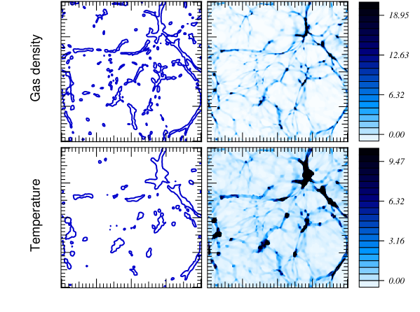
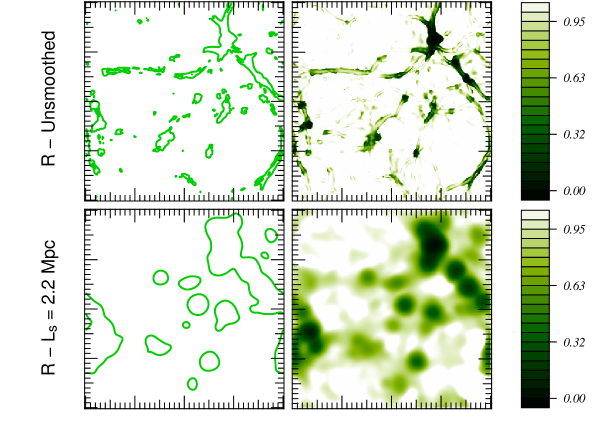
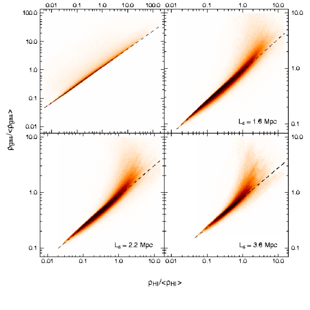
To illustrate this, Fig. 5(a) displays the gas density distribution (top), with its network of filaments outlined in the left panel with a contour corresponding to $\delta=1$, and the temperature distribution in units of $10^{4}$ K (bottom) for which we have drawn the contour corresponding to $(T/10^{4})=2$ in the left panel. Note that along filaments and at their intersection the gas is hot. This indicates that shock waves propagate along filaments, rising the temperature and ionizing the gas. This is confirmed by Fig. 5(b) which shows the ratio $R={\tilde{\rho}_{\rm HI}}/\rho_{\rm gas}$ measured directly in the $256^{3}$ grid (top), and after a Gaussian smoothing with a window whose size is $L_{\rm s}=2.2$ Mpc (bottom). In both cases, the panels on the left show the contours relative to $R=0.7$. To complete the picture, let us consider Fig. 6 which shows the scatter between $\rho_{\rm gas}$ and ${\rho}_{\rm H{\sc i}}$ for different smoothing scales, as indicated in each panel. As expected, the tightness of the correlation is very high in underdense and moderately dense regions, but shock heating on the one hand and the formation of condensed objects on the other produce a significant scatter (where $R<1$) along densest filaments and at their intersection (in clusters). For the purpose of the reconstruction, some smoothing is required. Unfortunately, smoothing also mixes these regions with the un-shocked part of the intergalactic medium. This is confirmed, in a qualitative way, by the slices shown in Fig. 5(b). More quantitatively, for the fields $R$ shown in Figure 5(b) we have calculated the fraction of the volume occupied by the regions with $R<0.7$ (i.e. the volume of the regions enclosed by the contours in the left panels). For the slice shown, this fraction is $f(R<0.7)=0.07$ and $f(R<0.7)=0.19$ for the un-smoothed and the smoothed case respectively, while when the whole three dimensional boxes are considered, the fraction of volume occupied by shocked regions are $f(R<0.7)=0.05$ and $f(R<0.7)=0.11$. As a result of such mixing, the tightness of the correlation is weakened, but remains good as shown in Fig. 6. However, the best fit values of the parameters $A$ and $\alpha$ changes slightly when the field is smoothed (see Table 1). We fit these values with the low density tail of the PDF (see Figure 3). As expected, the higher density tail match worsens with smoothing.

$L_{\rm s}$	$A$	$\alpha$
Unsmoothed	1.275	0.63
1.6 Mpc	0.915	0.56879
2.2 Mpc	0.85	0.55209
3.6 Mpc	0.795	0.5389

Table 1: Values of the parameters A and $\alpha$ entering in the scaling relation between gas and Hi (see Eq. 7) as a function of the smoothing scale $L_{\rm s}$.

Given that the scaling relation (7) is monotonous, should it apply exactly, the topology of the neutral gas should be exactly the same as of the total gas/matter distribution. However, given the dispersion of this relation, one expects the Euler characteristic of the $\tilde{\rho}_{\rm H{\sc i}}$ field to depart from that of $\rho_{\rm gas}$ for large density contrasts. This is confirmed by Fig. 4: a nearly perfect agreement is found between the gas and Hi for $\delta\la 0$, while differences become significant at larger values of the density contrast. Increasing the smoothing length (i.e. going from left to right in Fig. 4) worsens the match, as expected, but this is in part lost in the noise due to finite volume effects. Note that $\chi^{+}$ measured in Hi is, in the $\delta>0$ regime, more peaked than for the total gas. This agrees with intuition, since galaxies form in filaments: in these highly condensed objects, gas concentrates and cools down. Hence the Hi density becomes significant again inside these clumps, but is depleted in their surroundings due to shock heating as can be seen from Fig. 5. The resulting distribution of Hi in filaments is therefore expected to be more clumpy than the total gas i.e. less efficiently connected, resulting in a larger increase of $\chi^{+}$ for $\delta>0$. The estimates made inside filaments are however certainly not free of numerical artefacts since they are limited by the simulation’s spatial resolution (following accurately the formation of condensed objects requires much higher spatial resolution than our simulation). Therefore although one can definitely trust the $\delta\la 0$ measurements, the results derived for $\delta>0$ are likely to yield the right qualitative behavior, but are certainly quantitatively biased.

In the next Sections, the $\delta>0$ disagreement will be ignored and it will be assumed that the scaling relation (7) is always valid, keeping in mind the limitation of such an assumption. Hence, reconstructions will be performed on the optical depth without attempting to directly recover the gas distribution.

Figure 7: The effect of redshift distortion on the HI density. The same slice (whose width is 6 pixels, corresponding to 0.94 Mpc) of the Hi density contrast is shown without distortion (left panels) and with distortion (right panels, using the infinitely distant observer approximation with a distortion along the $x$ axis) in the case where the fields are not smoothed (top panels) and when the fields are smoothed at $L_{\rm s}=1.6$ Mpc (bottom panels).

Figure 8: Effect of redshift distortion on the Euler characteristic of Hi at different smoothing scales: $L_{\rm s}=1.6$ Mpc, 2.2 Mpc and 3.6 Mpc. The solid black line is for Hi without any distortions, the dashed yellow line has been obtained by including only the effect of peculiar velocities, while for the red thin line both redshift distortion and thermal broadening are taken into account.

3.2.2 From Hi to optical depth: redshift space distortions and thermal broadening

In the above discussion we argued that the main features of dark matter topology, as traced through the Euler characteristic and the probability density function, can be recovered through the topology of the Hi  for small density contrasts, $\delta\la 0$. However, along a line-of-sight, the optical depth is in fact observed in redshift space, where distortions induced by the peculiar motions operate. Moreover, the profiles of absorption lines are broadened at small scales by the effect of the temperature. Since the thermal broadening is important only at scales of the same order or smaller than the Jeans length, this second effect should be negligeable in the scaling range considered in this paper, since it will be swept out by the smoothing. On the contrary, redshift distortion should a priori not be neglected.

In theory, it is possible to partially correct for redshift distortion effects (see for instance PVRCP). However, the corresponding treatment of the peculiar velocities involves a simultaneous deconvolution of the Hi density field with the velocity field on top of the inversion discussed in next section. This requires not only a prior for the density field but also for its correlation with the peculiar velocity field and makes the inversion quite convolved and this would go beyond the scope of this paper. In what follows, it is shown that in fact redshift distortions have a small effect on the topology of the overall density distribution for the probed scales; they shall thus be neglected in the reconstruction part of this work. Moreover, one of the interesting outcomes of the reconstruction is to predict the positions of filaments in the three dimensional matter distribution. Cross-correlation of such a distribution with for instance the observed distribution of galaxies at high redshift can in fact be also performed in redshift space.

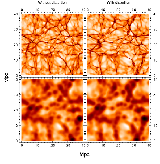
Figure 7 displays the Hi distribution in real and redshift space with and without smoothing: the main effect of redshift distortion on Hi is an enhancement of large scale density contrasts orthogonally to the line of sight due to large scale motions (this is the so-called Kaiser effect, e.g. Kaiser 1987): the “voids” (underdense regions) are more pronounced, and the filaments orthogonal to the LOS are more contrasted. There is as well a small scale “finger of god” effect, due to internal motions inside large dark matter haloes, but it is not very pronounced at such a high redshift, and is in amplitude of the same order of thermal broadening. Note however, that non trivial shell crossings can still occur, e.g. two filaments crossing each other thanks to peculiar velocities, but this effect remains small, and is clearly damped out by smoothing; after smoothing only the Kaiser effect remains.

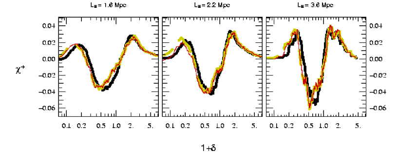
These qualitative arguments are illustrated by Figure 8. The measured Euler characteristics before and after redshift distortion differ only slightly. When the redshift distortion is taken into account, for $\delta\la 0$, a shift towards the left is induced (dashed curve) as compared to the non-distorted case (solid one); while the opposite occurs for $\delta\ga 0$ (although in the latter case, the effect seems to be nearly insignificant). This shift remains quite small as argued before. Note as well that thermal broadening (thin curve) is totally negligeable.

Finally, one last point should be mentioned. When one considers real absorption spectra, instrumental noise has to be taken into account in the analysis. This noise, combined with saturation of the flux of the Ly-$\alpha$ absorption lines arising in high density regions (with $\delta\ga 10$) can complicate the interpretation of the measurements. In this case, some of the information about the intensity of the density field cannot be recovered, unless, say, Lyman-$\beta$ is also available. In this work, however, the main interest lays in reproducing the low-density part of the Hi distribution, for which the relation (7) holds and for which the topology of the underlying dark matter distribution is theoretically constrained. In this regime, the Ly-$\alpha$ lines are not saturated, thus a complete treatment of saturation effects in high density regions is not required for the aim of the present work.

4 Topological and statistical properties of the recovered fields

The absorption spectrum towards a quasar gives access to one-dimensional information i.e. the optical depth along the line of sight (LOS) towards the QSO. However, if a set of LOSs towards a group of quasars is available, the information along each LOS can be interpolated to construct a 3-dimensional optical depth field.

In this Section we first briefly outline the inversion technique implemented to recover the optical depth and describes how to set the parameters that enter the inversion procedure. We then check how the reconstruction performs by measuring various statistical quantities, in particular the PDF of the density field and its Euler characteristic. As argued in the previous Section, the focus is on the optical depth: no attempt is made to recover the gas or dark matter distribution directly. Thermal broadening, redshift distortion and effects of saturation or instrumental noise are neglected. Given these assumptions, studying the optical depth distribution is then equivalent to studying the Hi density distribution, $\rho_{H{\sc i}}$.

4.1 The inversion method: Wiener interpolation

The technique used to interpolate the optical depth field between lines of sight is described and discussed in details in PVRCP.

Let D be a 1-dimensional array representing the data set (i.e. the values of $\gamma_{\rm LOS}=\ln(\rho_{H{\sc i}})$ along the LOSs, which we assume to be parallel to each other); we call M the 3-dimensional array of the parameters that need to be estimated (here the values of $\gamma_{\rm 3D}=\ln(\rho_{H{\sc i}})$ in the 3-dimensional volume) by fitting the data. Wiener interpolation reads (see Eq. 20 of PVRCP), assuming the noise is uniform and uncorrelated,

$${\bf M}={\bf C_{\rm MD}}\cdot({\bf C_{\rm DD}}+{\bf N})^{-1}\cdot{\bf D}\,,$$ (8)

where ${\bf N}=n^{2}{\bf I}$ is the diagonal noise contribution, ${\bf C_{\rm MD}}$ is the mixed parameters-data covariance matrix and ${\bf C_{\rm DD}}$ is the data covariance matrix:

$${\bf C_{\rm MD}}={\bf C_{\gamma_{\rm 3D}\gamma_{\rm LOS}}}\,,\quad{\bf C_{\rm DD}}={\bf C_{\gamma_{\rm LOS}\gamma_{\rm LOS}}}\,.$$ (9)

Here an ad-hoc prior is used and a Gaussian shape for the covariances is assumed. In this cases the matrices ${\bf C_{\gamma_{\rm 3D}\gamma_{\rm LOS}}}$ and ${\bf C_{\gamma_{\rm LOS}\gamma_{\rm LOS}}}$ are given by

$${\bf C}(x_{1},x_{2},{\bf x_{1\perp}},{\bf x_{2\perp}})=\sigma^{2}\times\exp\Big{(}-\frac{(x_{1}-x_{2})^{2}}{L_{x}^{2}}\Big{)}\times$$

$$\exp\Big{(}-\frac{|{\bf x_{1\perp}}-{\bf x_{2\perp}}|^{2}}{L_{T}^{2}}\Big{)}\,,$$ (10)

where $(x_{i},{\bf x}_{i\perp})$ represents the coordinates of the points along and perpendicular to the LOSs respectively, $L_{x}$ and $L_{T}$ are correlation lengths along and perpendicular to the LOSs, while $\sigma^{2}$ quantifies the typical a priori fluctuations in a volume of size $L_{x}\times L_{T}^{2}$. The meaning and choice of these parameters will be discussed further in § 4.2.

Note that the shape of the covariance matrix can be calculated with a more sophisticated approach. This would involve the use of theoretical priors relying on our knowledge of large scale structure dynamics. If, for instance, the reconstruction was performed on the pure dark matter density contrast, one could be tempted to derive these correlation matrices from the non-linear power spectrum obtained, for example, by Peacock & Dodds (1996), given a cosmological model. Here, a simpler interpolation scheme is used. This scheme has the advantage of depending only on three tuning parameters: the assumed typical overall signal-to-noise ratio, $\sigma/n$, and two typical lengths in the interpolation, $L_{x}$ and $L_{T}$.

4.2 Choice of the parameters in the interpolation

Each reconstruction is performed on a number $N_{\rm LOS}$ of LOSs extracted at random from the simulation box. Since the distant observer approximation is implemented, all the LOSs are parallel. For a given value of $N_{\rm LOS}$, the mean inter-LOS distance, $\langle d_{\rm LOS}\rangle$, reads:

$$\langle d_{\rm LOS}\rangle\equiv\sqrt{L_{\rm box}^{2}/N_{\rm LOS}}.$$ (11)

This parameter obviously defines a natural scale in the reconstruction: one cannot, intuitively, expect to reconstruct details of the distribution at scales $\la\langle d_{\rm LOS}\rangle$, at least in the direction orthogonal to the LOSs.

The meaning of the parameters $L_{T}$ and $L_{x}$ in Eq. (10) is then quite straightforward. The correlation lengths $L=L_{T}$ and $L=L_{x}$ stabilize the inversion by ensuring the smoothness of the reconstruction. In order to avoid the formation of fictitious structures, the transverse correlation length must be of the order of the mean separation between the LOSs, $L_{\rm T}\sim\langle d_{\rm LOS}\rangle$ (we have chosen to take it exactly equal to $\langle d_{\rm LOS}\rangle$), while the choice of the longitudinal correlation length depends on the problem considered. Since redshift distortion is not a concern in the present work, this parameter can be chosen to be of the order of the Jeans length in order to avoid information loss for small scales along the LOSs, here $L_{x}=0.4$ Mpc.

Raw fields

Smoothed fields in logarithmic space                                            Smoothed fields in linear space

Figure 9: Qualitative comparison between the original Hi density field in terms of $\gamma=\ln(1+\delta)$ (left column in each group of 4 panels) and the recovered one (right column in each group of 4 panels) in a thin slice (the thickness of the slice is 8 pixels, corresponding to 1.25 Mpc). Higher densities correspond to darker colors. The recovered field has been obtained by inverting a set of $N_{\rm LOSs}=320$ random LOSs (mean separation $\langle d_{\rm LOS}\rangle=2.24$ Mpc) taken through the original (unsmoothed) density field. In each group of panels, the first row corresponds to a slice orthogonal to the LOSs, while the second row corresponds to a slice parallel to the LOSs. Upper group: the raw $\gamma$ fields for the original box and for the reconstruction. Lower left group: same as the upper group but after smoothing (in the logarithmic space) with a Gaussian window of radius $L_{\rm s}=\sqrt{2}\langle d_{\rm LOS}\rangle=3.17$ Mpc. Lower right group: same as the lower left one, but smoothing is now applied directly to the density field, $1+\delta=\exp(\gamma)$, instead of its logarithm and the normalization is slightly different (see Eq. 15 of Appendix A).

From a practical point of view, the variance parameter $\sigma$ of the correlation matrix fixes the relative contribution of signal to noise in Eq. (8), $\sigma/n$. In our reconstruction, only ideal LOSs are considered. Thus, strictly speaking, there is no instrumental noise or saturation effects. However, the inversion of the matrix ${\bf C_{\rm DD}}+{\bf N}$ is numerically unstable when ${\bf N}$ is set to zero, given the finite sampling and the degeneracy of the matrix, Eq (10), close to its diagonal, $(x_{1},{\bf x_{1\perp}})\simeq(x_{2},{\bf x_{2\perp}})$. In practice one has to “tune” the signal-to-noise ratio, $\sigma/n$, to obtain the best compromise between numerical stability and “exactness” of the final reconstruction. This choice is ad-hoc: $(\sigma/n)^{2}$ is the estimated variance $\sigma^{2}(L_{T},L_{x})$ of the underlying field in a box of size $L_{T}\times L_{T}\times L_{x}$. This is equivalent to assuming that, as the noise goes to zero, the inverse of the non-reduced second order correlation (in the appropriate units) is used, ${\bf I}+{\bf C}_{\rm DD}$, instead of the reduced one, ${\bf C}_{\rm DD}^{-1}$, to perform a stable reconstruction.

In this work we estimate directly $\sigma^{2}(L_{T},L_{x})$ from the simulation. It is however important to note that $\sigma^{2}(L_{T},L_{x})$ can in principle be derived from the LOSs alone by measuring the 1-D power-spectrum of $\rho_{H{\sc i}}$. From this 1-D power-spectrum, one can indeed infer a 3-D power-spectrum with standard deconvolution methods and then an estimate of $\sigma^{2}(L_{T},L_{x})$ by the appropriate integral on the 3-D power-spectrum.

The measured values of $\sigma(L_{T},L_{x})$ are listed in Table 2. They are of the order unity: the assumed signal-to-noise ratio is about one in the regime considered here. Hence, in practice, the ad-hoc procedure used to perform the inversion does not change significantly by including the contribution of the actual instrumental noise. However, in this case the presence of the saturated regions in the Lyman-$\alpha$ spectra remains a problem.

$N_{\rm LOS}$	Separation	$L_{T}$	$\sigma$
	(arcmin)	(Mpc)
400	1.33	2	1.12
320	1.49	2.24	1.17
225	1.77	2.67	1.23
200	1.88	2.83	1.25
145	2.2	3.32	1.29
120	2.42	3.65	1.31
100	2.65	4	1.34

Table 2: Parameters used in the reconstructions performed in this paper. The longitudinal correlation length as been fixed to the value $L_{x}=0.4$ Mpc for all the reconstructions.

Finally, note that due to the large size of the matrices, reconstructions can only be performed by partioning the simulation box in blocks of smaller size, that contain $N_{\rm sub}^{3}$ grid points with $N_{\rm sub}=32$. The reconstruction is performed on each block individually. In order to avoid edge effects, neighboring patches are overlapped by adding a buffer region in which LOSs still contribute. In this way, the a priori correlation ensure continuity between adjacent patches. The size of the buffer region is chosen to be $n_{\rm over}\simeq 2L_{T}$ (in grid pixel units), which implies a typical residual contamination of edge effects due to the partitioning of less than 2 percent.

4.3 Bias in the reconstruction

Figure 10: Statistics and topology in logarithmic space, i.e. in terms of $\gamma_{H{\sc i}}=\ln(1+\delta_{H{\sc i}})$, for three different reconstructions performed with $N_{\rm LOS}=320$, $N_{\rm LOS}=200$ and $N_{\rm LOS}=120$, from left to right respectively. First row of panels: the power-spectrum of $\gamma_{H{\sc i}}$ as a function of wavenumber indicated at the top. In each panel, the thin dashed curve represents the power spectrum of the original field while the thick solid line is the power spectrum of the (unsmoothed) recovered field. The light shaded region corresponds to the scatter between five realizations of Gaussian fields (GRFs) with the same power spectrum as the reconstruction. The wavenumber $k$ is expressed in unit of the inverse of the pixel size multiplied by $2\pi$, corresponding roughly to $k\simeq 1/L({\rm Mpc})$. Second row of panels: the probability distribution function as a function of $\gamma_{H{\sc i}}=\ln(1+\delta_{H{\sc i}}$ (as it is indicated at the bottom), after smoothing $\gamma_{H{\sc i}}$ with a Gaussian window of size $L_{\rm s}=\sqrt{2}\langle d_{\rm LOS}\rangle$. Solid thick and dashed thin lines correspond to the recovered and the original fields, respectively. The light shaded region in each panel represents the scatter derived from the five GRFs, while the big dots correspond to gaussian profiles with same mean and same variance as the smoothed recovered fields. Third row of panels: similarly as for the second row, but for the Euler characteristic. Fourth row of panels: similarly as for the third row, but for the individual critical point counts. In that case, the thick and thin lines correspond to the recovered and original fields, respectively. The solid, dashed, dotted and dot-dashed lines correspond respectively to minima, pancake saddle points, filament saddle points and maxima.

Figure 11: Left panel: Comparison between the skeletons of the original field (light lines) and its recovered counterpart (darker lines) (the skeletons represented here are the true ones, and not their local approximations, as defined in the main text). The original field was recovered by inverting $N_{\rm LOS}=320$ lines of sight, corresponding to a separation $\langle d_{\rm LOS}\rangle=2.24$ Mpc. Both skeletons are computed on fields smoothed over a scale $L_{\rm s}=3.16$ Mpc, in logarithmic space. For clarity, only a $4$ Mpc slice is shown, the background contour representing the original smoothed density field (lighter colors corresponding to higher densities). Right panel: Evolution of the inter-skeleton distance (ISD) between the original and reconstructed fields as a function of the number of line of sight $N_{\rm LOS}$. The ISD is computed after smoothing over a scale $L_{\rm s}=3.65$ Mpc which is roughly equivalent to the lowest resolution reconstruction sample. The upper (crosses) and lower (squares) curves represent the measured median distance from the reconstructed field skeleton to the original one and vice versa respectively, while the dotted curve represent their average value.

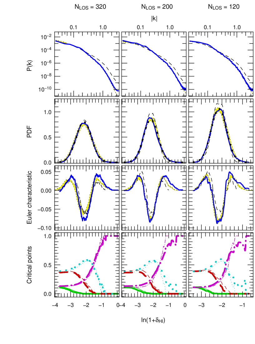
First note that the inversion is not directly performed on the density, but on its logarithm, i.e. the normalized density field is written as $\rho_{H{\sc i}}=1+\delta_{H{\sc i}}\equiv\exp(\gamma_{H{\sc i}})$ and the field $\gamma_{H{\sc i}}$ is interpolated by using the method described above. This has two advantages: (i) it ensures the positivity of the reconstructed density; (ii) since the density turns out to be roughly log-normal (see for example Bi & Davidsen, 1997; Choudhury, Padmanabhan & Srianand, 2001; Viel et al., 2002a; Zaroubi et al.; 2006, Desjacques et al., 2007; and see Coles & Jones, 1991, for the statistical properties of the log-normal distribution), performing the reconstruction on the logarithm of the field is expected to reproduce more realistic results as shown on Fig. 3.

However, as a result of the reconstruction, the recovered field, $\gamma_{H{\sc i},\rm rec}$, will be smooth over anisotropic volumes of size $\sim L_{x}\times L_{T}\times L_{T}$, which means that at best, one can identify structures at this level of smoothness on a logarithmic space. Although theoretical predictions (namely gravitational clustering, primordial non Gaussianities, etc. ) do exist for the density field itself, that is for $\rho_{H{\sc i}}=\exp(\gamma_{H{\sc i}})$ and its smoothed counterparts, they can not be applied directly in our case because smoothing and taking the exponential are operations which do not commute, except in the weakly nonlinear regime, $\delta_{H{\sc i}}\ll 1$. In particular, recovering the results for $\delta_{H{\sc i}}$ on a linear space, by taking the exponential of $\gamma_{H}{\sc i}$ and subsequently smoothing it, an effective bias, essentially due to rare peaks in the $\gamma_{H{\sc i},\rm rec}$ field, is introduced. The effect of such a nonlinear bias is difficult to control and can in some cases be important as shown below and studied in more details in Appendix A.

Figure 12: Variance (top panel) and skewness (bottom panel) of $\gamma_{H{\sc i}}=\ln(1+\delta_{H{\sc i}})$ for the original (open crosses), the recovered (filled crosses) fields and the Gaussian prediction (light dots), as functions of the LOS separation, $\langle d_{\rm LOS}\rangle$. The symbols correspond to measurements performed on the $\gamma$ fields smoothed with a Gaussian window of size $L_{\rm s}=\sqrt{2}\langle d_{\rm LOS}\rangle$. For a proxy of the errorbars, we used the measurements at smoothing scales $L_{\rm s}=\langle d_{\rm LOS}\rangle$ and $L_{\rm s}=\sqrt{3}\langle d_{\rm LOS}\rangle$, except for the Gaussian fields, where the dispersion among the 5 realizations is a better choice. For the Gaussian case, the skewness should be exactly zero. The measurements are consistent with that value, despite the large dispersion at the largest scales, due to finite volume effects.

Figure 13: Same as in Fig. 12 but for the filling factor of underdense regions at the minimum of the Euler characteristic. The Gaussian limit, not shown here, would give a filling factor exactly equal to 0.5.

Figure 14: Contours of underdense regions estimated from the minimum of the Euler characteristic in logarithmic space. The thick curves represent the contours for two recovered fields $\gamma_{H{\sc i},{\rm rec}}$ obtained by the inversion of $N_{\rm LOS}=320$ and $N_{\rm LOS}=200$ lines of sight (solid and dashed lines respectively). Prior to contour determination, the recovered field was smoothed with a Gaussian window of size $L_{\rm s}=\sqrt{2}\langle d_{\rm LOS}\rangle$. These contours should be compared with those of the original field, $\gamma_{H{\sc i}}$, represented with a thin line, smoothed at the same scales (solid and dashed lines respectively). This figure is complemented with the two upper panels of the lower left group shown in Fig. 9, where the same slices for the original and the recovered fields are displayed.

Figure 15: Same as Fig. 14, but smoothing is performed in linear space. This figure is complemented with the two upper panels of the lower right group in Fig. 9, where the same slices for the original and the recovered fields are displayed.

4.4 Testing the reconstruction: statistical and topological analysis

We now test the quality of the reconstruction using the same statistical tools as in Section 3, namely the PDF of the field and the Euler characteristic. Other statistics are considered, such as the variance and the skewness of the PDF, the power-spectrum of the density field and the filling factor of regions less dense than the minimum of the Euler characteristic. In addition, to have a quantitative estimate of the accuracy in the locus of the filamentary structures, we use the skeleton as introduced by Novikov, Colombi & Doré (2006) and by Sousbie et al. (2007) and define an inter-skeleton distance (ISD).

Following the discussion in Section 4.3, the reconstruction is mainly tested on the field $\gamma_{H}{\sc i}$ and its smoothed counterparts. In Appendix A we provide additional results on the field $\delta_{H{\sc i}}$.

Since there are two scales in the inversion (see Section 4.2), the recovered optical depth is an anisotropic smooth field with fewer structures in the direction transverse to the LOSs than in the direction parallel to them. Optimal comparison between reconstructed and real optical depth would require an approach based on anisotropic smoothing, a level of complexity well beyond the scope of this paper. Instead, to compare the reconstructions to the exact solution, an isotropic smoothing via a Gaussian window is used (see Eq. 5). The width of the smoothing window is $L_{\rm s}\ga\langle d_{\rm LOS}\rangle=L_{T}$. The choice of the optimal smoothing scale is constrained by the inter-skeleton distance.

One of the uncertainties in the reconstruction involves the determination of the mean value of the field $\mu_{\rm true}\equiv\langle\gamma_{H{\sc i}}\rangle\equiv\langle\ln\rho_{H{\sc i}}\rangle$, which can in principle be estimated only along the LOSs. To improve the quality of the reconstruction, its average is fixed to $\mu_{\rm true}$:

$$\gamma_{H{\sc i},\rm rec}={\tilde{\gamma}}_{H{\sc i},\rm rec}-\langle{\tilde{\gamma}}_{H{\sc i},\rm rec}\rangle+\mu_{\rm true}.$$ (12)

In practice, the knowledge of $\mu_{\rm true}$ is expected to be accurate, even though its actual measured value, $\mu_{\rm LOS}$, is determined along the LOSs. For instance in the worse case considered in this work, $N_{\rm LOS}=100$, $\langle(\mu_{\rm LOS}-\mu_{\rm true})^{2}\rangle^{1/2}/|\mu_{\rm true}|\simeq 1.91\%$, where the mean value of the difference between the measured and the real $\mu$ has been calculated by averaging over 100 different realizations of 100 LOSs.

4.4.1 Visual inspection

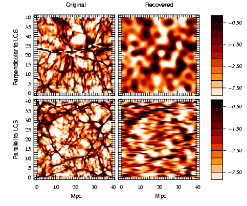
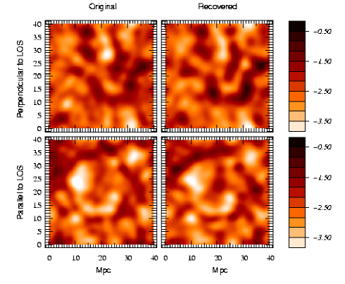
A first qualitative comparison between the original and the recovered fields in logarithmic space can be made by examining Figure 9. The top panels illustrate the anisotropic nature of the reconstruction. Smoothing at a scale $L_{\rm s}\ga\langle d_{\rm LOS}\rangle$ (for example, in the case of Fig. 9, $L_{\rm s}=\sqrt{2}\langle d_{\rm LOS}\rangle$), greatly improves the agreement between the reconstruction and the exact solution and the two field become almost indistinguishable (bottom left panels). When one examines in detail where the reconstruction fails, one notices that these structures correspond to overdense regions. The fine nature of the web formed by overdense regions (filaments, clusters) makes the reconstruction more difficult for these regions than for the underdense ones because of the sparse sampling of the transverse structures.

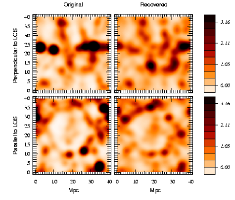
When going to linear space, i.e. taking the exponential of the fields and subsequently smoothing them, the effect caused by the amplification of rare events discussed in § 4.3 becomes obvious, as illustrated by the bottom right panels of Figure 9, that represent the counterpart of the bottom left panels in linear space. In logarithmic space the highest density peaks are highly depleted, here they are visible and spread over a beam the typical size of which is that of the smoothing window.

4.4.2 Power-spectrum: the scales correctly reconstructed

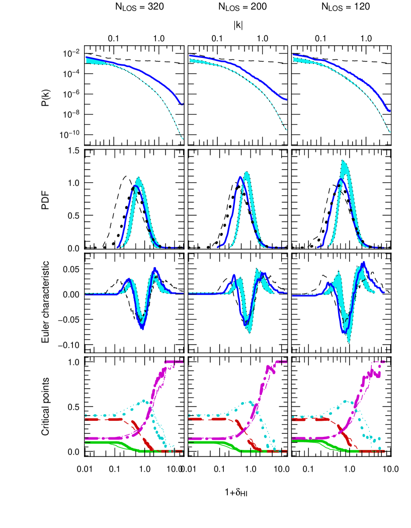
The good agreement between the original and the recovered fields in logarithmic space is confirmed by the first row of panels in Fig. 10, which shows the power-spectrum, $P(k)=\langle|\gamma_{\bf k}|^{2}\rangle$, of the raw fields, $\gamma_{H{\sc i}}$ and $\gamma_{H{\sc i},\rm rec}$, for three reconstructions ($N_{\rm LOS}=320,\ 200,\ 120$, corresponding respectively to $\langle d_{\rm LOS}\rangle=2.24$, $2.83$ and $3.65$ Mpc). We also show five realizations of a Gaussian random field (GRF) with the same $P(k)$ as $\gamma_{H{\sc i},\rm rec}$, in order to estimate finite volume effects. As expected, the filtering nature of the reconstruction introduces an apodization effect on $P(k)$ visible on Fig. 10: a bending of $P(k)$ is expected to happen roughly for $k\simeq k_{\rm bend}\equiv 2\pi/L_{\rm T}$, i.e., $k_{\rm bend}=0.44$, $0.35$, $0.27$ from the upper left to the upper right panel, respectively, in the units chosen in Fig. 10. It is not straightforward to check accurately this property by visual inspection. Indeed, when $N_{\rm LOS}$ decreases, the small $k$ part of the reconstructed power-spectrum becomes less well correlated with the true $P(k)$, giving the illusion, for example, that overall the $N_{\rm LOS}=120$ reconstruction does better than the $N_{\rm LOS}=320$ one. Still for $k\la k_{\rm bend}$, i.e., $L_{\rm s}\ga L_{\rm T}=\langle d_{\rm LOS}\rangle$, there is a good agreement between the reconstruction and the exact solution. However, the measurement of the power-spectrum itself is not accurate enough neither does it contain enough information to guarantee that filaments are well reconstructed in detail, as we examine now.

4.4.3 The skeleton: optimal smoothing scale

The visual inspection of Figure 9 seems to show that the filamentary pattern of the overall three-dimensional distribution is well recovered by the reconstruction in logarithmic space. One can check that assertion more quantitatively on the skeleton (Novikov et al., 2006; Sousbie et al., 2007). This will allow us to define an optimal smoothing scale which will be used in the subsequent analyses. More detailed analyses relying on the skeleton are postponed to another paper.

The actual definition of the skeleton is in fact deeply related to the Euler characteristic since it relies on first principles of Morse theory: basically, the skeleton is composed of the set of field lines (the curves defined by the gradient of the density field) starting from the filament saddle points ($I=2$ in the formalism described in § 2.1) and converging to local maxima. Although apparently simple, solving this equation is quite difficult, this is why a local approximation, based on a Taylor expansion around the critical points contained in the skeleton, was introduced in Novikov et al. (2006) and extended in 3D by Sousbie et al. (2007): the local skeleton. In this paper we use the implementation of Sousbie et al. (2007).

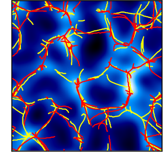
Note that, as opposed to a global topological estimator such as the Euler characteristic, the skeleton provides a local test of the accuracy of reconstruction (i.e., one can check whether a precise filament at a given location is recovered or not). Figure 11 presents the skeleton (yellow lines) of a $4$ Mpc slice extracted from the original Hi density field, as well as the skeleton of its reconstructed counterpart (red lines), using $320$ LOSs. Both fields are smoothed in logarithmic space using a gaussian window of scale $L_{\rm s}=3.16$ Mpc. This figure confirms that, on large scales, the general shape of the filamentary structures is well preserved, demonstrating the ability of the reconstruction to recover the cosmic web. Nonetheless, as expected, some discrepancies appear on small scales.

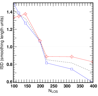
The inter-skeleton distance (ISD) is an estimator which allows to make a quantitative comparison. A skeleton corresponds to a number of small segments linked together to form the filaments. In order to estimate the average distance between two skeletons, A and B, for each segment of A, the distance to the closest segment in B is computed leading to the PDF of the distribution of the spatial separation from A to B. The distance from A to B is defined as the median of this PDF. Since this definition of distance is not symmetrical (in the sense that ISD(A,B) and ISD(B,A) will, in general, be different), the mean distance between A and B is defined as the average of these quantities. Figure 11 presents the measurement of the ISD between the skeleton of the original field and its reconstruction, as a function of the number of LOSs used to perform the inversion (in units of the smoothing scale). In all cases, both fields were smoothed over a scale $L_{\rm s}=3.65$ Mpc. What is important to notice here is the sharp transition at $N_{\rm LOS}=225$, corresponding to $L_{\rm s}=L_{\rm crit}$ with

$$L_{\rm crit}\simeq 1.35\langle d_{\rm LOS}\rangle.$$ (13)

For a smoothing scale $L_{\rm s}\la L_{\rm crit}$, the match between reconstruction and exact solution worsens suddenly, while no significant improvement is really seen when $L_{\rm s}\ga L_{\rm crit}$: $L_{\rm crit}$ represents some “optimal” smoothing scale, which is the smallest possible scale at which the reconstruction performs well, in terms of filamentary pattern recovery. Note that only the measurements for a particular value of $L_{\rm s}$ are shown, but Eq. (13) should not change significantly for the scaling range considered in this work.

Although all the subsequent analyses involving smoothing were performed at various scales, namely $L_{\rm s}^{2}=\langle d_{\rm LOS}\rangle^{2}$, $2\langle d_{\rm LOS}\rangle^{2}$, $3\langle d_{\rm LOS}\rangle^{2}$, increasing likewise the number of LOSs contributing per smoothing volume, we shall, in light of the above findings, mainly concentrate on the results corresponding to $L_{\rm s}^{2}=2\langle d_{\rm LOS}\rangle^{2}\simeq L_{\rm crit}^{2}$.

4.4.4 Statistical analysis

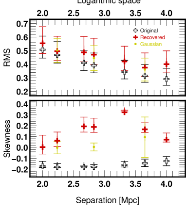
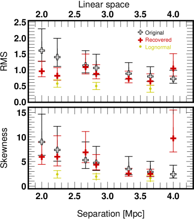
The second row of Fig. 10 shows the PDFs of the smoothed counterparts of $\gamma_{H{\sc i}}$ (dashes) and $\gamma_{H{\sc i},\rm rec}$ (solid), with a window of size $L_{\rm s}=\sqrt{2}\langle d_{\rm LOS}\rangle$, as argued just above. These measurements are supplemented with Fig. 12, which shows the variance and the skewness of the PDFs of various fields as functions of separation between the LOSs. Again, the agreement between the solid and dashed curves in second row of panels of Fig. 10 is quite good and the results do not depend significantly on the value of $N_{\rm LOS}$.

From a quantitative point of view, the difference between the recovered and the original curves can be calculated using the following estimator,

$${\rm err}=\frac{\sum_{i}|y_{i}^{\rm orig}-y_{i}^{\rm rec}|\Delta x_{i}}{\sum_{i}|y_{i}^{\rm orig}|\Delta x_{i}}\,,$$ (14)

where $y_{i}^{\rm orig}=y^{\rm orig}(x_{i})$ and $y_{i}^{\rm rec}=y^{\rm rec}(x_{i})$ are the values of the curves relative to the original and the recovered fields respectively and the curves have been sampled at points $x_{i}$. This corresponds to the area between the curves, normalized by the area enclosed by the original ones. For the three reconstructions shown, the errors are of the order of ${\rm err}_{\rm PDF}=10-20\%$.

These quantitative estimates show that there are still some noticeable differences between the reconstruction and the true field: the shape of PDF of the reconstructed field, $\gamma_{H{\sc i},\rm rec}$, tends to be Gaussian, within the error range provided by the five Gaussian fields. This “Gaussianisation” is expected from both the central limit theorem and the shape of the correlation matrix given by Eq. (10). Note that this statement is not totally consistent with the measurement of the skewness (lower panel of Fig. 12), especially at intermediate separations between the LOSs. However, this skewness is quite sensitive to the upper tail of the PDF corresponding to rare events in overdense regions: one expects, in that regime, deviations from Gaussianity in the reconstruction because the central limit is not yet reached.

The true field, $\gamma_{H{\sc i}}$, deviates slightly from a Gaussian, as already shown in Fig. 3. In particular, in the right part of the bell shape of the PDF on Fig. 10, there is a slight disagreement between the dashed and the continuous curves, which corresponds to the weak negative skewness measured in lower panel of Fig. 12. This disagreement would be even more visible if a logarithmic representation were used on the $y$ axis to display the PDF: the high density tail of the Hi field is far from lognormal. The main contribution to such a tail comes from collapsed objects in clusters and in filaments. As argued in § 4.4.1, these objects are sparsely sampled by the LOSs, which worsens the quality of the reconstruction in overdense regions.

4.4.5 Global topology

The nearly Gaussian nature of the reconstructed $\gamma$ field can be also confirmed by examining the third row of panels in Fig. 10, which is similar to the second row, but displays the Euler characteristic as a function of the density threshold. Deviations from Gaussianity of the true field, $\gamma_{H{\sc i}}$, are more clearly visible than for the PDF. In particular, on all the panels, the corresponding dashed curve always presents an asymmetry between its two maxima, contrary to what is observed in the Gaussian limit. The reconstruction, $\gamma_{H{\sc i},\rm rec}$, being more symmetrical, is clearly closer to the Gaussian limit than the true field. However, as noticed earlier for the skewness of the PDF, one cannot really claim that the reconstruction is fully Gaussian: deviations outside the range allowed by our five Gaussian realizations are noticeable, particularly in the right panel and in general in the overdense right tail ($\gamma\ga-1.5$) of $\chi^{+}$. Still the overall topology of the reconstructed field, although closer to the Gaussian limit, reproduces rather well the topology of the true field, especially in the range $-2.0\la\gamma\la-1.5$, which confirms the findings of § 4.4.3 on the skeleton. This density regime is indeed dominated by filaments saddle points and local maxima, as shown by the last row of panels of Fig. 10, which displays the different critical point counts as functions of the density threshold for $\gamma_{H{\sc i}}$ and $\gamma_{H{\sc i},{\rm rec}}$ . Note the increasing contribution of the noise when $N_{\rm LOS}$ decreases, which makes the agreement between reconstruction and exact solution worse, particularly for large densities, as expected. From a more quantitative point of view, one can, similarly as for the PDF, compute the integrated errors on the critical point counts (Eq. 14). For the 3 reconstructions we consider here, these errors are of the same order as for the PDF (i.e. less than 20%).

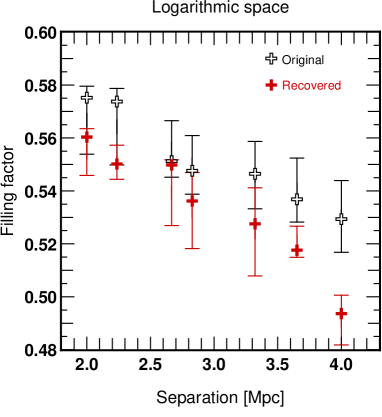
As an additional test, the minimum of the Euler characteristic, $\gamma_{\rm min}\sim-2$, can be used to define a topological boundary between “underdense” and “overdense” regions. Indeed in the Gaussian limit, this minimum lies exactly at $\gamma_{\rm min}=\langle\gamma\rangle$. Defining the filling factor of underdense regions, $FF_{\rm underdense}$, as the fraction of space occupied by points verifying $\gamma\leq\gamma_{\rm min}$, one expects $FF_{\rm underdense}$ to be always close to $0.5$: at least this is true for any monotonic local transform of a Gaussian field (with no additional smoothing). Even though the reconstruction and the true field do not have exactly the same behavior for $\chi^{+}$, they seem to have very close values of $\gamma_{\rm min}$, which should correspond to a good agreement between the measured values of $FF_{\rm underdense}$: this is indeed the case as shown in Fig. 13. Although the measured values of $FF_{\rm underdense}$ are consistent with those of the original ones, the connectivity of the underdense (or equivalently, overdense) regions defined in this way is good but not perfect, as illustrated by Fig. 14. In this range of densities, connectivity of the excursion is controlled equally by filament and pancake saddle points and their respective counts tend to be slightly underestimated and overestimated, respectively, as illustrated by bottom panels of Fig. 10. This is however not enough to explain the discrepancies in Fig. 13, and shows the limits of global topological estimators.

At the qualitative level, note finally that the situation becomes worse when one attempts to recover the boundary contour between overdense and underdense regions in linear space, because of the bias mentioned in § 4.3. This is shown in Figure 15, which represents the same slice as in Figure 14 but in this case the contours were calculated from the minimum of the Euler characteristic after smoothing the exponential of the fields. Here, the position of the structures in the recovered contours is significantly different from that of the original fields, not to mention connectivity. Appendix A, which discusses a figure similar to Fig. 10 but in linear space, fully confirms these results.

5 Discussion and conclusion

In this paper we have studied the topology of large scale structures as traced by the intergalactic medium (IGM) in a hydrodynamical cosmological simulation. The main goal was to test a reconstruction method (PVRCP) of the three-dimensional large scale matter distribution from multiple lines of sights (LOSs) towards quasars. For this purpose, we relied on a number of global statistical tools, the probability distribution function of density field (PDF), the Euler characteristic ($\chi^{+}$) as an alternate critical point counts and related quantities such as the variance and the skewness of the PDF, the individual critical points counts and the filling factor of the underdense regions at the minimum of the Euler characteristic. We also used the skeleton as local probe of the geometry and the topology of the field. The main results of our investigations can be summarized as follows

• In the first part of this paper we addressed the problem of relating the topology of the dark matter density field to the topology of the distribution traced by the total amount of gas and the neutral gas (Hi). When one considers the Hi density distribution at scales larger than the Jeans length of the gas and takes into account the IGM equation of state relating the neutral and total amount of gas, then the properties of this nearly lognormal distribution are exactly the same as found for the dark matter/total gas in underdense regions (i.e. for density contrasts $\delta\la 0$). For larger density contrasts, some deviations appear, due to shocks (where Hi is depleted) and to the presence in filaments and clusters of highly condensed objects (where Hi is very concentrated). Taking these results into account, with the additional assumption that instrumental noise, in particular effects of saturation, can be neglected, we have shown that studying the topological properties of large scale matter density distribution is equivalent to studying directly those of the optical depth or in what follows, those of neutral gas, Hi.

• In the second part of this work we tested the Wiener interpolation proposed by PVRCP to recover the three-dimensional distribution of Hi from a set of multiple LOSs, along which the (one-dimensional) distribution of Hi is assumed to be known exactly. This interpolation depends on three parameters, the typical size, $L_{x}$ of structures along the LOSs, the typical mean LOSs separation, $L_{T}=\langle d_{\rm LOS}\rangle$, and the expected variance of the fluctuations of the field which can be in principle indirectly inferred from the LOSs themselves.

  Our investigation shows that the reconstruction method can be used to predict quite accurately the patterns in the large scale matter distribution at scales of the order of $\sim 1.4\langle d_{\rm LOS}\rangle$ or larger when one attempts to recover the logarithm of the density field. In particular it allows us to recover the position of filaments in the large scale distribution: we compared the skeleton of the initial and recovered field and measured the distance between these skeletons and found that for smoothing scales larger than $\sim 1.4\langle d_{\rm LOS}\rangle$, the inter-skeleton distance remains smaller than $\langle d_{\rm LOS}\rangle$. Furthermore, the global shape of the PDF, of the fraction of critical points and of the Euler characteristic are well reproduced, the integral errors on these quantities varying in the range 10-20%. Discrepancies between the reconstruction and the exact solution are mainly found in overdense regions, where deviations from a lognormal behavior are the most significant.

The good recovery of the statistical properties of the density field in logarithmic space, is strongly related to the Gaussian prior on which the inversion method is based. Recall that, since the distribution of the gas density is very close to log-normal, the distribution of its logarithm is well approximated by a Gaussian function. As demonstrated in PVRCP, the Wiener interpolation is just a special case of the maximum likelihood method. It gives, under the hypothesis that the statistical distributions of the data and of the parameters are Gaussian, the optimal reconstruction for a linear model. However, this relies on a proper knowledge of the covariances matrices. Here we assume a simple functional shape for these matrices, given by Equation (10). A better treatment would need an accurate knowledge of the underlying power-spectrum of the logarithm of the density. The interpolation could for instance be improved by using a stronger prior relying on the extension of e.g. the nonlinear ansatz of Hamilton et al. (1991) to logarithmic space.

We noticed that some deviations are present in the original field, compared to the log-normal limit at the scales we have probed here. This information could be added to the model. This could be achieved by applying an Edgeworth expansion to the logarithm of the field [Juszkiewicz et al. 1995, Colombi 1994], hence by taking into account slight deviations of the likelyhood function from a Gaussian distribution to correct our Wiener interpolator (Amendola, 1998).

Even though the best variable for the reconstruction is the logarithm of the density, theoretical predictions are usually performed on the density itself. Therefore it is in practice difficult to compare the properties of the reconstructed density distribution to those predicted by e.g. nonlinear perturbation theory (e.g. Bernardeau et al. 2002) or other models. The problem is that linear space gives more emphasis to rare events in overdense regions. In Appendix A we analyse the corresponding bias on the reconstruction, and find that it is critical for the higher density peaks. As a result, the tomography is in practice much less robust when expressed directly in linear space. However, this is mainly related to the fact that our analyses are performed at scales smaller or of the order of 4 Mpc, where non-linear effects in the dynamics are still present.

Due to the size of our simulation ($L_{\rm box}=40$ Mpc), in this work we have analysed the properties of connectivity at relatively small scales ($L_{\rm s}=4$ Mpc), where the distribution of matter is close to log-normal. However, one could in principle extend the analyses to larger scales, to probe the linear or quasi-linear regime, where the density distribution is actually close to Gaussian. In that case, the reconstruction should be performed on the density itself rather than on its logarithm while the above mentioned problems would become irrelevant. In particular, the implementation of the improvements on the Wiener interpolator could for instance be used to test directly if non trivial deviations from Gaussianity are present or not in the data. If present, they could be ascribed to primordial non-gaussian features that are produced during the inflationary phase or as a result of topological defects.

The inversion method is based on the hypothesis that a sufficiently strong correlation exists at the scale under consideration. Indeed, various sources of noise can hide such a correlation completely (errors due to the finite cosmological volume probed by a finite number of LOSs, noise in the measurement of the spectra), making the reconstruction irrelevant. To test the strength of the correlation a large number of quasar pairs spanning the range of separations we want to probe must be observed. It has been recently shown [Coppolani et al. 2006] that at $z\approx 2$ for a separation of $\sim 5$ arcmin (corresponding to $\approx 7.6$ Mpc for a flat universe with $\Omega_{\rm m}=0.3$, $\Omega_{\Lambda}=0.7$ and $H_{0}=70\,{\rm km}\,{\rm s}^{-1}\,{\rm Mpc}^{-1}$), some correlation is observed, suggesting that the inversion method could be applied at such scales. It is thus very important to measure more accurately the transverse correlation function from quasar pairs. Indeed, once this is done, we can include this information as a self-consistent prior in the reconstruction procedure.

Using realistic data about the luminosity function of quasars [Jiang et al. 2006], it is found that for magnitude limits of $g\mbox{$\>\stackrel{{\scriptstyle<}}{{{}_{\sim}}}\>$}(23,24,25)$ the number of quasars observed per square degree at $z\mbox{$\>\stackrel{{\scriptstyle>}}{{{}_{\sim}}}\>$}2$ is $n_{\rm QSOs}=(41,77,136)$ respectively. For the set of cosmological parameters assumed here, the corresponding mean angular separations are $\langle d_{\rm LOS}\rangle=(9.37,6.84,5.15)$ arcmin. Moreover, for $g\mbox{$\>\stackrel{{\scriptstyle>}}{{{}_{\sim}}}\>$}23$ the number density of Lyman-break galaxies (LBGs) starts to become significant and we can think of using these objects as background sources in combination with QSOs. In particular, it is found that for $g\mbox{$\>\stackrel{{\scriptstyle<}}{{{}_{\sim}}}\>$}(23,24,25)$ the number of LBGs par square degree is $n_{\rm LBGs}=(0.3,116,2325)$ respectively [Adelberger & Steidel 2000], so that, even at $g\mbox{$\>\stackrel{{\scriptstyle<}}{{{}_{\sim}}}\>$}24$, the number of available sources is largely increased. In Table 3 we display the mean separation one can expect as a function of the magnitude limit.

Magnitude limit	Separation (QSOs)	Separation (QSOs et LBGs)
$g$	(arcmin)	(arcmin)
23	9.4	9.3
24	6.8	4.3
25	5.2	1.2

Table 3: Mean angular separation between the background sources as a function of the magnitude limit (left column).

One can see that if we are able to observe objects up to a magnitude limit of $g\sim 24$, the density of background sources will be high enough to perform a reconstruction similar to what described in this paper. A better approach will be to search for peculiar fields in which the density is larger by chance (e.g. Petitjean 1997). The spectral resolution will be a decreasing function of the magnitude. Observational difficulties will include the contamination of the LBG spectrum by absorption lines originating in the interstellar medium of the galaxy and the fact that the mean redshift ($z\approx 2.8$) will be larger than what we have considered in this paper. To reach these faint magnitudes we need to wait for the advent of the Extremely Large Telescopes (Theuns & Srianand 2006).

To conclude, the approach developed here is very promising as the advent of Extremely Large Telescopes will boost this field by allowing the observation of a number of background sources large enough to probe the distribution of the matter with accurate precision at the scales under consideration. The total amount of observing time will be large however but worthwhile given the expected results foreseen in this paper.

Appendix A Recovered field: analysis in linear space

Figure 16: Same as in Fig. 10, but in the linear space, i.e. by taking the exponential of the recovered fields and the Gaussian realizations along with normalization 15, with subsequent smoothing with a Gaussian of size $L_{\rm s}=\sqrt{2}\langle d_{\rm LOS}\rangle$ for the last three row of panels. The big dots on the second row of panels now correspond to a lognormal distribution with same variance and average as the reconstruction.

While the reconstruction seems to perform well for $\gamma=\ln(\rho)$ and its smoothed counterparts (except that it is somewhat “Gaussianized”, as shown by the measurements in the main text), let us now investigate what happens for the statistical properties of the field itself $\rho=\exp(\gamma)$.

It was noted in that case (§ 4.3) that the recovered field is expected to be biased, originating from the fact that taking the exponential of a field does not commute with smoothing via a Gaussian window. Furthermore, taking the exponential gives emphasis to high density peaks, which are the most poorly reconstructed (§ 4.4). Additional smoothing contaminates neighboring pixels as well, resulting in significant changes in the connectivity. These effects were confirmed at the qualitative level in the main text by visual inspection of Figs. 9, 14 and 15. We now examine them more quantitatively.

Figure 17: Same as Figure 12, but in linear space, as explained in caption of Fig. 16.

Figure 18: Same as Fig. 13, but in linear space, as explained in caption of Fig. 16.

As just argued above, since we are working in linear space, $\rho\sim\exp(\gamma)$, rare events in overdense regions (which are poorly reconstructed) dominate. As a consequence, the reconstruction fails with respect to the mean density: equation (12) is clearly not appropriate anymore to normalize the reconstruction. Instead, the reconstructed density, $\rho_{H{\sc i},\rm rec}$, is renormalized as follows:

$$\rho_{H{\sc i},{\rm rec}}=\langle\rho_{H{\sc i}}\rangle\frac{\exp({\tilde{\gamma}}_{H{\sc i},\rm rec})}{\langle\exp({\tilde{\gamma}}_{H{\sc i},\rm rec})\rangle},$$ (15)

where $\langle\rho_{H{\sc i}}\rangle$ is the true mean density in the simulation. Note that this density is no longer accurately determined from direct measurements on the LOSs: in the worse case considered in this paper, $N_{\rm LOS}=100$, we indeed find a relative error on the estimate of $\langle\rho_{H{\sc i}}\rangle$ of the order of $30$%. However, the simulation volume is quite small, leading to unrealistically short LOSs. In real observations the determination of the average neutral gas density along LOSs should be much more accurate [Guimar es et al. 2007].

The choice of the normalization given by Eq. (15) is natural since it imposes the average density of the reconstructed field to be equal to that of the exact solution. However, because it is still affected by overdense regions contributions, this normalization is not fully satisfactory as it does not lead to the appropriate corrections in underdense regions, as can be noted by a careful examination of 4 lower right panels of Fig. 9.

The contamination by high density peaks affects all statistics, as illustrated by Figs. 16 and 17. This is particularly dramatic for second order statistics (upper row of Fig. 16 and upper panel of Fig. 17). The reconstruction underestimates the normalization of the power-spectrum, and as a result the variance of the PDF, especially when the separation between the LOSs is small: in the latter case, nonlinear features in the density field are given more weight and are poorly captured by the reconstruction. This appears as a shift in the PDF shown in the second row of panels in Fig. 16, worsening with increasing $N_{\rm LOS}$. Note however that the agreement between the reconstruction and the exact solution, although poorer than in logarithmic space, improves when $N_{\rm LOS}\la 200$. Note also that the smoothed lognormal fields no longer match the reconstruction. In fact, in the linear space, its seems that the reconstruction gives a solution intermediate between the exact one and the smoothed lognormal fields, both from the point of view of the power-spectrum and the PDF (and its cumulants) (Fig. 17): it captures more than just the Gaussian features of the logarithm of the real solution, as would have naively followed from the analysis of § 4.4.

These results are confirmed in the third row of panels in Fig. 16: the measured Euler characteristic of the reconstruction gives an intermediate solution between the true and the lognormal solution (see for instance the position of the local extrema of the curves representing $\chi^{+}$). Note that overall, the reconstruction matches better the lognormal behaviour than the true solution, especially when $N_{\rm LOS}$ is large, implying that “lognormalization” dominates, at least from a topological point of view, while nonlinear dynamics implies significant departures from a purely lognormal behavior. This explains again why the quality of the reconstruction decreases when attempting to probe the smallest scales. Note that this does not mean that decreasing the number of LOSs is better: the analysis always looks at the smallest scale recoverable in logarithmic space, $\sim 1.4\langle d_{\rm LOS}\rangle$. At fixed smoothing scale, a reconstruction with a given number of LOSs does better than a reconstruction with sparser LOS sampling. Still, note that the reconstruction does more than a simple “lognormalization” as it gives an intermediary answer between the expected lognormal behavior from the analysis in logarithmic space and the true solution, at least from the point of view of the PDF and the Euler number. The uncertainties in the measurements due to the emphasis put on rare events are however too large to drive definite conclusions with a small sample of LOS: the spread between the five lognormal fields is much larger than they were in the logarithmic space (and similarly for the PDF).

Let us finally check the global topological properties of the reconstruction by examining the number counts of each kind of critical points individually, as shown in the last row of panels in Figure 16. Notwithstanding all the above points, note that the inversion achieves a fair reconstruction of the distribution of some of the critical points: in the low density regime, it overestimates the local minima count, as expected from visual inspection of four lower right panels of Fig. 9 and from the PDF: the reconstructed field in underdense region is overestimated. In the intermediate density range, reconstruction overestimates pancake saddle point counts (and to a lesser extent, underestimates filaments saddle point and local maxima counts) for $N_{\rm LOS}=320$ while larger separations between LOSs do better. In the overdense regime, where the reconstruction fails more dramatically, and where the amplification of the errors is large, one tends to overestimate (underestimate) filament saddle points (local maxima).

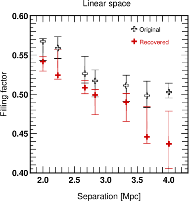
Still, it is interesting to note that the local minimum of the Euler number, $\rho_{\rm min}\sim 0.7$ is comparable for the reconstruction and the exact solution, suggesting that the measured filling factor defined previously will be similar for the reconstruction and the exact solution: according to Figure 18, the filling factor of underdense regions at the minimum of the Euler number does nearly as well as in logarithmic space, but the match between its isocontours is worse than before (compare Figure 14 with Figure 15): thus, even if the critical point counts and the fraction of underdense regions agree, this does not necessarily imply that the structures, in particular the densest ones, are at the right position.

References

- [Adelberger & Steidel 2000] Adelberger, K. L., Steidel, C. C., 2000, ApJ, 544, 218
- [Amendola 1998] Amendola, L., 1998, astro-ph/9810198
- [Aracil et al. 2002] Aracil, B., Petitjean, P., Smette, A., Surdej, J., Mücket, J.P., Cristiani, S., 2002, A&A, 391, 1
- [Bardeen et al. 1986] Bardeen, J. M., Bond, J. R., Kaiser, N., Szalay, A. S., 1986, ApJ 304, 15
- [Bernardeau et al. 2002] Bernardeau, F., Colombi S., Gaztañaga, E., Scoccimarro, R., 2002, Physics Reports 367, 1
- [Bi & Davidsen 1997] Bi, H. G., Davidsen, A. F., 1997, ApJ, 479, 523
- [Cen et al. 1994] Cen, R., Miralda-Escudé, J., Ostriker, J., P., Rauch, M., 1994, ApJ, 437, L9
- [Choudhury et al. 2001] Choudhury, T. R., Padmanabhan, T., Srianand, R., 2001, MNRAS, 322, 561
- [Coles & Jones 1991] Coles, P., Jones, B.,1991, MNRAS, 248, 1
- [Colombi 1994] Colombi, S., 1994, ApJ, 435, 536
- [Colombi et al. 1994] Colombi, S., Bouchet, F. R., Schaeffer, R., 1994, A&A, 281, 301
- [Colombi et al. 2000] Colombi, S., Pogosyan, D., Souradeep, T., 2000, PhRvL, 85, 5515 (CPS)
- [Coppolani et al. 2006] Coppolani, F., Petitjean, P., Stoehr, F., Rollinde, E., Pichon, C., Colombi, S., Haehnelt, M., Carswell, B., Teyssier R., 2006, MNRAS, 370, 1804
- [Croft et al.1998] Croft, R.A.C., Weinberg, D.H., Katz, N., Hernquist, L., 1998, ApJ, 495,44
- [Crotts & Fang 1998] Crotts, A.P.J., Fang, Y., 1998, ApJ, 502, 16
- [Davé et al. 2001] Davé et al. 2001, ApJ, 552, 473
- [Desjacques et al. 2007] Desjacques, V,, Nusser, A., Sheth, R. K., 2007 MNRAS, 374, 206
- [Doroshkevich 1970] Doroshkevich, A. G. 1970, Astrophysics, 6, 320
- [Gnedin & Hui 1998] Gnedin, N. Y., Hui, L., 1998, MNRAS, 296, 44
- [Gott et al. 1986] Gott III, J. R., Melott, A. L., Dickinson, M. 1986, ApJ, 306, 341
- [Gott et al. 1987] Gott III, J. R., Weinberg, D. H., Melott, A. L., 1987, ApJ, 319, 1
- [Guimar es et al. 2007] Guimar es, R., Petitjean, P., Rollinde, E., de Carvalho, R. R., Djorgovski, S. G., Srianand, R., Aghaee, A., Castro, S., 2007, MNRAS, 377, 657
- [Gunn & Peterson 1965] Gunn, J. E., Peterson, B. A. 1965, ApJ, 142, 1633
- [Guzzo 2001] Guzzo, L. 2001, astro-ph/0102062
- [Hamilton et al. 1991] Hamilton, A. J. S.; Kumar, P.; Lu, Edward; Matthews, Alex 1991, ApJ, 374, 1L
- [Hui et al. 1999] Hui, L., Stebbins, A., Burles, S. 1999, ApJ, 511, L5
- [Jiang et al. 2006] Jiang, L., Fan, X., Cool, R. J., Eisenstein, D. J., Zehavi, I., Richards, G. T., Scranton, R., Johnston, D., Strauss, M. A., Schneider, D. P., Brinkmann, J., 2006, AJ, 131, 2788
- [Juszkiewicz et al. 1995] Juszkiewicz, R., Weinberg, D. H., Amsterdamski, P., Chodorowski, M., Bouchet, F., 1995, ApJ, 442, 39
- [Kaiser 1984] Kaiser, N. 1984, ApJ, 284, L9
- [Kaiser 1987] Kaiser, N. 1987, MNRAS, 227, 1
- [McDonald & Miralda-Escudé 1999] McDonald, P., Miralda-Escudé, J. 1999, ApJ, 518, 24
- [Mecke, Buchert & Wagner 1994] ecke, K. R., Buchert, T., Wagner, H., 1994, A&A 288, 697
- [Milnor, Morse Theory] Milnor, 1963, Morse Theory p.29
- [Miralda-Escudé et al. 1996] Miralda-Escudé, J., Cen, R., Ostriker, J. P., Rauch, M., 1996, ApJ, 417, 582
- [Mucket et al. 2004] Mucket, J. P., Petitjean, P., Kates, R. E., Riediger, R. 1996, A&A, 308, 17
- [Nakagami et al. 2004] Nakagami, T., Matsubara, T., Schmalzing, J., Jing, Y., 2004, astro-ph/0408428
- [Novikov et al. 2006] Novikov, D., Colombi, S., Doré, O., 2006, MNRAS, 366, 1201
- [Nusser & Haehnelt] Nusser, A., Haehnelt, M., 1999, MNRAS, 303, 179
- [Park et al. 2005] Park, C., Choi, Y., Vogeley, M. S., Gott III, J. R., Kim, J., Hikage, C., Matsubara, T., Park, M., Suto, Y., Weinberg, D. H., 2005, ApJ, 633, 11
- [Peacock & Dodds 1996] Peacock, J. A., Dodds S. J., 1996, MNRAS, 280, L19
- [Petitjean et al. 1995] Petitjean, P., Mücket, J. P., Kates, R. E., 1995, A&A, 295, L9
- [Petitjean 1997] Petitjean, P., 1997, euvl.conf, p266, (arXiv:astro-ph/9608115)
- [Petitjean et al. 1998] Petitjean, P., Surdej, J., Smette, A., Shaver, P., Mücket, J., Remy, M. 1998, A&A, 334, L45
- [Pichon et al. 2001] Pichon, C., Vergely, J. L., Rollinde, E., Colombi, S., Petitjean, P., 2001, MNRAS, 326, 597 (PVRCP)
- [Protogeros & Weinberg 1997] Protogeros, Z. A. M., Weinberg, D. H., 1997, ApJ, 489, 457
- [Rauch 1998] Rauch, M., 1998, ARA& A, 36, 267
- [Rollinde et al. 2001] Rollinde, E., Petitjean, P., Pichon, C., 2001, A&A, 376, 28
- [Rollinde et al. 2003] Rollinde, E., Petitjean, P., Pichon, C., Colombi, S., Aracil, B., D’Odorico, V., Haehnelt, M. G. 2003, MNRAS, 341, 1299
- [Schmalzing & Buchert 1997] Schmalzing, J., Buchert, T., 1997, ApJ, 482, L1
- [Sousbie et al. 2006] Sousbie, T., Pichon, C., Courtois, H., Colombi, S., Novikov, D., 2006, submitted to ApJLett. (arXiv:astro-ph/0602628)
- [Sousbie et al. 2007] Sousbie, T., Pichon, C., Colombi, S., Novikov, D., Pogosyan, D. 2007, submitted to MNRAS (arXiv:astro-ph/0707.3123)
- [Spergel et al. 2007] Spergel, D. N., Bean, R., Doré, O., Nolta, M. R., Bennett, C. L., Dunkley, J., Hinshaw, G., Jarosik, N., Komatsu, E., Page, L., Peiris, H. V., Verde, L., Halpern, M., Hill, R. S., Kogut, A., Limon, M., Meyer, S. S., Odegard, N., Tucker, G. S., Weiland, J. L., Wollack, E., Wright, E. L., 2007, ApJS, 170, 377
- [Theuns et al. 1998] Theuns, T., Leonard, A., Efstathiou, G., Pearce, F.R., Thomas, P. A., 1998, MNRAS, 301, 478
- [Theuns & Srianand 2006] Theuns T. & Srianand R., 2006, IAUS, 232, 464 (arXiv:astro-ph/0601637v1)
- [Trac et al. 2002] Trac, H., Mitsouras, D., Hickson, P., Brandenberger, R., 2002, MNRAS, 330, 531
- [Viel et al. 2002a] Viel, M., Matarrese, S., Mo, H. J., Haehnelt, M. G., Theuns, T., 2002, MNRAS, 329, 848
- [Viel et al. 2002b] Viel M., Matarrese S., Mo, H. J., Theuns T., Haehnelt M. G. 2002, MNRAS, 336, 685
- [Viel et al. 2004] Viel, M., Haehnelt, M. G., Springel, V., 2004, MNRAS, 354, 684
- [Viel et al. 2006] Viel, M., Haehnelt, M. G., Springel, V., 2006, MNRAS, 367, 1655
- [Vogeley et al. 1994] Vogeley, M. S., Park, C., Geller, M. J., Huchra, J. P., Gott III, J. R., 1994, ApJ, 420, 525
- [Young et al. 2001] Young, P. A., Impey, C. D., Foltz, C. B. 2001, ApJ, 549, 76
- [Zaroubi et al. 2006] Zaroubi, S., Viel, M., Nusser, A., Haehnelt, M., Kim, T. S., 2006, MNRAS 369, 734