Risk-Seeking vs. Risk-Avoiding Investments in Noisy Periodic Environments

J. E. Navarro B., F. E. Walter, F. Schweitzer

1 Introduction

In the course of this paper, we investigate a model in which agents with different strategies participate in an simple investment scenario with noisy returns [NavarroEtAl07]. We use this setup to approach the question how the (internal) complexity of agents enhances their performance in a hard-to-predict environment. In the field of artificial intelligence and complex systems, one can distinguish between two types of agents: first, agents which only react on external changes (also known as “zero-intelligence agents” [Gode-Sunder93, Farmer-Patelli04]) and second, agents which have a complex internal architecture (e.g. “belief-desire-intention agents”). Despite these clear differences in agent architecture, it is difficult to determine what influence these properties have on the overall performance of the agents. In order to study this question in a controlled environment, we have chosen an investment model with noisy returns, to compare the performance of simple and complex agents. To which extent is worthwhile to equip an agent with complex learning mechanisms instead of having a reactive response to exogenous returns?

As a necessary step to study more complex scenarios, we are interested in an initial study of the performance of different agent architectures/investment strategies in the following simple setup: each agent has a certain budget $x(t)$ and is able to invest a certain fraction of its budget on a market. The gain or loss it makes depends on the market return, or return on investment (RoI). In other words, at each time step $t$, the agent adjust its risk propensity, the fraction of its budget that it are willing to invest on the market, denoted by $q(t)$, thereby controlling gains and losses resulting from the RoI, denoted by $r(t)$. We assume that only the past and current values of $r(t)$ are known to the agent; it does not know the dynamics governing future values of $r(t)$. Agents observe the market through the value of $r(t)$ and, based on analysing a set of past $r(t)$ values, they predict future $r(t)$ values and determine their behaviour on that market through specifying $q(t)$.

In this simple model, we consider agents that invest independently in the market, i.e. there is no interaction or communication with other agents. Also, there is no feedback of the investments done by agents on the market return. In other words, the environment of the agents is not influenced by their investments. This is a crucial assumption which makes our model different from other attempts to model real market dynamics, e.g. as for financial markets [LeBaron01, Lux-Marchesi02, Raberto-Cincotti03]. Consequently, we do not construct and investigate a market model; rather, our focus lies on investigating what are good and what are bad strategies – in a rather artificial and controlled market environment (see also Section 4). Regarding the relevance of our results for real financial markets, see also our comments in the concluding Section 7.

(a)                                                      (b)

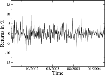
Figure 1: (a) Real returns of a stock item (in this example, the stock was AAA, the Altana Group) in percent over time (01/05/2002 – 01/03/2004). $r(t)$ was computed for a current price $p(t)$ as follows: $r(t)=\log{p(t)}-\log{p(t-1)}$. (b) The dynamics of the market as indicated by the market return $r(t)$ and the strategy as defined by the invested budget $q(t)$. Note that our model does not consider the feedback of investments on the market dynamics (dashed line).

The essence of the model is captured in Figure 1: (a) plots the returns in percent of a real stock item over the range of about two years. This illustrates the range and shape of values of returns of a real-world stock item. (b) illustrates the dynamics of the model: $r(t)$, the market return, influences the strategies agents have to adjust $q(t)$, the risk propensity. In this particular model, we do not consider the influence that adjusted risk propensity has on the market return, i.e. the influence of $q(t)$ on $r(t)$.

The challenge for the agents thus is twofold: first, agents have to predict $r(t)$ as accurately as possible, and second, they have to adjust $q(t)$ to the proper values as quickly as possible. This is a complex and difficult task since most investment environments are uncertain and fluctuating. Choosing to avoid risk and investing too little may lead to small gains, and choosing to take risk and investing too much may lead to large losses.

The task of finding an appropriate strategy that controls the risk and balances between these two extrema is by far not trivial. Methods from technical analysis, such as estimations based on moving averages or moving least squares (see also Section 3.2) try to approximate the behaviour of the environment and, based on that approximation, determine the most appropriate investment at a particular time. In the theory of risk, several authors assume that individuals choose among assets based on the mean return and on the variance of the return [markowitz91, maslov98, kirman05]. Others have focused their attention to the important task of how to measure risk, which lead to different type of measures [pratt64, Artzner99]. In general, these measures are based on the risk aversion of a decision maker having the choice to receive a random or a non-random amount.

A typical scenario to study investment strategies is to let an agent choose between investing in a risk-free asset or in a risky asset[tobin58, pratt64]. It was shown[tobin58] that sometimes it may be more reasonable to invest in a risk-free asset as a means to transfer wealth over time. However, assuming a model with no consumption [hens06], those agents investing in risk-free assets will be driven out of the market in the long run by agents investing in a risky asset. When dealing with risky assets, it is typically assumed that the agent considers the expected return and its volatility as indicators for the investment strategy [markowitz91].

For the sake of simplicity, in this paper we assume that the agent’s behavior is risk-neutral in the sense that the agent estimates only the expected return, $r(t)$, and does not consider risk measures such as the volatility. Based on the estimation of $r(t)$, the decision to increase or decrease the investment fraction of the risky asset should be taken. Hence, the two terms ’risk-seeking’ and ’risk-avoiding’ refer only to the choice of the investment fraction, $q(t)$.

The remainder of this paper is organised as follows: In the next section, Section 2, we present the details of the investment model, the properties and abilities of an agent acting/investing in this environment. Following that, Section 3 presents some of the strategies that an agent can use to control its risk propensity and Section 4 presents the properties of the return on investment (RoI) that we are considering; Section 5 illustrates the optimal parameter adjustment for the presented strategies and their derivation; Section 6 compares the different investment strategies. This is done by means of simulations where the average total budget of agents using each investment strategy is obtained for a large a number of trials. Finally, in Section 7, we present our conclusions.

2 Model

In this model, agents are characterised by the following two variables:

1. their budget $x(t)$, which is a measure of their “wealth” or “liquidity”, and

2. the strategy that they employ in order to control the fraction of the budget $q(t)$ to invest at each time step.

In other words, at each time step $t$, an agent invests a portion $q(t)x(t)$ of its budget. The investment yields a gain or a loss, determined by the value of $r(t)$. Being a fraction of the investment budget, $q(t)$, is, of course, restricted to the interval between $[0,1]$. However, in our model we further restrict it to be from the interval $[q_{min},q_{max}]$ where we choose $q_{min}=0.1$ and $q_{max}=1.0$. This implies that, at each time step $t$, there is a minimal investment of $0.1$ of the budget, and a maximal investment of the entire budget.

We can then define the dynamics for the budget of agents $x(t)$ as

$$x(t+1)=x(t)\,\Big{[}1+r(t)\,q(t)\Big{]}$$ (1)

where $r(t)$ is the market return at the previous time step $t$. The market return function $r(t)$ is restricted to the range of $[-1,1]$. A value of $r(t)=-1$ corresponds to a total loss of the invested fraction of the budget $q(t)$ and $r(t)=1$ corresponds to a gain equivalent to the invested fraction. Thus, an agent can, at any time step $t$, loose its complete budget (for $q(t)=1$ and $r(t)=-1$), but also double its budget (for $q(t)=1$ and $r(t)=1$). In principle, there is no upper boundary for $r(t)$, $r(t)=1$ was chosen to obtain a mean of zero for $r(t)$ which allows us to better understand the basic dynamics of this model. We emphasize again that, in our model, the aim is not a most realistic simulation of the market return, but a comparison of different agent strategies. The difficulty for the agents lies in properly predicting the next value of $r(t)$ and then adjusting $q(t)$ fast enough.

Note that the restriction of $r(t)$ to the range of $[-1,1]$ is not a realistic assumption for a real market. There, some $r(t)$ will also fall into the range $)-1,1($ – these are rare, extreme events that occur, e.g. in cases of stock market bubbles and crashes. However, normally, returns will be in the range of $[-1,1]$, e.g. as the ones of the stock depicted in Figure 1. As we would like to focus on the questions of choosing appropriate agent strategies in environments with noisy, periodic returns, it is reasonable to exclude such rare, extreme events and assume a restriction of $r(t)$ to the range of $[-1,1]$.

In the next two sections, we will outline the agent strategies (Section 3) and return on investment (Section 4) that we consider.

3 Agent Strategies

As explained before, we are interested in how the market dynamics, $r(t)$, affect the different investment strategies of the agent, $q(t)$. It is very important to realise that the market dynamics – while affecting each agent’s $q(t)$ – are not known to the agents. I.e., at time $t$, each agent only receives the actual value of the Return on Investment (RoI) and adjusts its risk propensity accordingly, without having a complete knowledge about the dynamics of $r(t)$. The agent may, of course, have some bounded memory about past RoI that could be used for predictions of future RoI. However, the agent has to gather information about the ups and downs of the RoI and to draw its own conclusions from this information by itself. Therefore, the agent will perform better in the environment if it is able to guess the market dynamics.

In the following, we present a selection of strategies that can be applied by agents. We distinguish a reference strategy, which serves as a frame of reference to compare and evaluate the performance of other strategies, as well as technical analysis-based and machine learning-based strategies. Usually (there are exceptions, as will be discussed in the following), a strategy consists of two components: a prediction component and an action component. For such strategies, the prediction component predicts a variable in the system – in this case, the next value of $r(t)$ – and the action component then defines an action upon the prediction of the variable – in this case, it defines the appropriate value for $q(t)$.

3.1 Reference Strategy

In order to compare different strategies, we need a point of reference against which the performance of each strategy can be measured. The reference strategy that we are using is the most simple strategy possible, i.e. that an agent always assumes a constant risk-propensity value $q_{0}$ at every time step $t$:

$$q(t)=q_{0}=\mathrm{const.}$$ (2)

Since the value of $q(t)$ is always fixed, this is not really a “strategy”, but it plays a role in more physics-inspired investment models [Sornette-Cont97, Takayasu-Sato97, NavarroEtAl07]. We use this strategy to compare it with more complex strategies. Note that this reference strategy requires no knowledge on the RoI.

3.2 Technical Analysis

The following simple strategies for risk adjustment are based on “technical analysis” [Brooks02]. Technical analysis tries to deduce information about the dynamics of $r(t)$ by looking at trends (averages, variances, higher order moments) of the RoI values over a range of time. This assumes that an agent has a bounded memory of size $M$ to record previous RoI; this information is then processed in different ways to predict the next RoI. In the following, we consider two strategies from the field of technical analysis: the first strategy is based on calculating moving averages (MA) on previous RoI, while the second strategy uses moving least squares (MLS) on previous RoI, $r(t)$, over a fixed period of time, $M$. Both of them can be regarded as “zero-intelligence” strategies, as agents do not do any reasoning or learning.

3.2.1 Moving Averages

The moving averages technique computes $\hat{r}_{MA}(t)$, an estimate of the next $r(t)$, as the average of the previous $M$ values of $r(t)$:

$$\hat{r}_{MA}(t)=\frac{1}{M}\sum_{n=t-M}^{t-1}r(n)$$ (3)

3.2.2 Moving Least Squares

The moving least squares technique fits a function to the data of the previous $M$ values of $r(t)$ to estimate the next $r(t)$. In our case, we choose this function to be a linear trend-line, which is found by minimising the distance to the data points of $r(t)$. Based on the previous $M$ values of $r(t)$, the squared estimation error $\epsilon_{r}$ is defined as:

$$\epsilon_{r}(t)=\frac{1}{M}\sum\limits_{n=t-M+1}^{t}\left[r(n)-\hat{r}_{MLS}(n)\right]^{2}$$ (4)

where $\hat{r}_{MLS}(t)$ is the predicted RoI based on the linear regression trend-line, defined as:

$$\hat{r}_{MLS}(t^{\prime})=m(t)\,t^{\prime}+b(t)\quad\mathrm{for}\;t-M\leq t^{\prime}\leq t$$ (5)

Now, the best fitting values $m$ and $b$ are obtained by minimising the squared error estimation, eq. (4). From $\partial\epsilon_{r}/\partial m=0$ and $\partial\epsilon_{r}/\partial b=0$, we get, as it is well known:

$$m(t) = \frac{M\sum\limits_{n=t-M+1}^{t}n\,r(n)\;-\;\left(\sum\limits_{n=t-M+1}^{t}n\right)\left(\sum\limits_{n=t-M+1}^{t}r(n)\right)}{M\sum\limits_{n=t-M+1}^{t}n^{2}-\left(\sum\limits_{n=t-M+1}^{t}n\right)^{2}}$$ (6)

$$b(t) = \frac{1}{M}\left[\sum\limits_{n=t-M+1}^{t}r(n)-m(t)\sum\limits_{n=t-M+1}^{t}n\right]$$ (7)

These two strategies use different approaches to estimate future $r(t)$; it remains to define the corresponding adjustment of the risk propensity: here, we consider two possibilities. First, a risk-seeking (RS) and, second, a risk-avoiding (RA) approach. In the risk-seeking approach, the value of $q_{RS}(t)$ is defined as follows for $\hat{r}(t)\in\{\hat{r}_{MA}(t),\hat{r}_{MLS}(t)\}$, i.e. for $\hat{r}(t)$ being an MA or MLS estimate of $r(t)$:

$$q_{RS}(t)=\begin{cases}q_{\mathrm{\min}}&\textrm{$\hat{r}(t)\leq 0$}\\ q_{\mathrm{\max}}&\textrm{$\hat{r}(t)>0$}\end{cases}$$ (8)

where $q_{\mathrm{\min}},q_{\mathrm{\max}}\in[0,1]$ and $q_{\mathrm{\min}}<q_{\mathrm{\max}}$. In other words, agents invest $q_{\mathrm{\min}}$ if the next value of $r(t)$ is predicted to be negative or zero, and agents invest $q_{\mathrm{\max}}$ if the next value of $r(t)$ is predicted to be positive.

In the risk-avoiding approach, the value of $q_{RA}(t)$ is defined as follows for $\hat{r}(t)\in\{\hat{r}_{MA}(t),\hat{r}_{MLS}(t)\}$, i.e. for $\hat{r}(t)$ being an MA or MLS estimate of $r(t)$:

$$q_{RA}(t)=\begin{cases}q_{\mathrm{\min}}&\textrm{$\hat{r}(t)\leq q_{\mathrm{\min}}$}\\ \hat{r}(t)&q_{\mathrm{\min}}<\hat{r}(t)<q_{\mathrm{\max}}\\ q_{\mathrm{\max}}&\textrm{$\hat{r}(t)\geq q_{\mathrm{\max}}$}\end{cases}$$ (9)

where $q_{\mathrm{\min}},q_{\mathrm{\max}}\in[0,1]$ and $q_{\mathrm{\min}}<q_{\mathrm{\max}}$. Here, the respective $q(t)$ is set to the predicted $r(t)$ (with appropriate adjustments to ensure that $q(t)=q_{min}$ whenever $\hat{r}(t)\leq q_{min}$ and $q(t)=q_{max}$ whenever $\hat{r}(t)\geq q_{max}$) – agents only invest a fraction of the budget which corresponds in size to the expected return.

3.3 Machine Learning Approaches

Another class of strategies for risk adjustment is based on more complex agent information processing capabilities from the field of machine learning. In this paper, we consider two such approaches: one based on an incremental update rule (IUR), which is a form of reinforcement learning, and the other based on a genetic algorithm (GA), which is a form of evolutionary learning.

3.3.1 Incremental Update Rule

The following machine learning approach is based on the incremental update rule, an application of reinforcement learning [Sutton98]. The idea of reinforcement learning is that an agent continuously uses a reward signal to adjust its own performance. In our scenario, the values of the return are the reward signal; at each step, the agent computes the error between the predicted and the actual value of the return and uses this error to adjust the estimation of the following return. The general incremental update rule from reinforcement learning is defined as follows:

$$\textrm{\emph{NewEst}}\leftarrow\textrm{\emph{OldEst}}+\textrm{\emph{StepSize}}[\textrm{\emph{Target}}-\textrm{\emph{OldEst }}]$$ (10)

$OldEst$ and $NewEst$ are the old and new estimates for the quantity of interest. So, $Target-OldEst$ gives the error of the current estimation, which is weighted by the factor $StepSize$. This is, a new estimate is computed by taking the old estimate and adjusting it by the error of the current estimate. $NewEst$ has to be updated at each time step. Applying eq. (10) to our model, we find the following instance of the incremental update rule:

$$\hat{r}_{IUR}(t+1)=\hat{r}_{IUR}(t)+\gamma\bigl{[}r(t)-\hat{r}_{IUR}(t)\bigr{]}$$ (11)

Consequently, $OldEst$ and $NewEst$ are the old and new estimates for the return, $\hat{r}_{IUR}(t)$ and $\hat{r}_{IUR}(t+1)$; furthermore, $r(t)-\hat{r}_{IUR}(t)$ is the error of the current estimate. Because of its recursive definition, the incremental update rule considers an infinite history of returns – of course, the weight of a value depends on its age and its impact fades over time. We chose $\hat{r}_{IUR}(0)=0$ as the initial value of $\hat{r}_{IUR}(t)$. Different values of $\gamma$ lead to different performance of the algorithm; in other words, for small $\gamma$, the adjustment of the estimate will be small, and for large $\gamma$, the adjustment of the estimate will be large. It is important to choose an optimal value for $\gamma$ in order to be able to compare the algorithm with other algorithms; in the next section, we will discuss this in more detail. Finally, it remains to specify what action to do given a particular estimate for the next return; we again define a risk-seeking and a risk-avoiding approach, similar to eq. 8 and 9 for the MA and MLS strategies:

In the risk-seeking approach, $q_{RS}(t)$ is defined as follows for $\hat{r}_{IUR}(t)$:

$$q_{RS}(t)=\begin{cases}q_{\mathrm{\min}}&\textrm{$\hat{r}_{IUR}(t)\leq 0$}\\ q_{\mathrm{\max}}&\textrm{$\hat{r}_{IUR}(t)>0$}\end{cases}$$ (12)

and in the risk-avoiding approach, $q_{RA}(t)$ is defined as follows for $\hat{r}_{IUR}(t)$:

$$q_{RA}(t)=\begin{cases}q_{\mathrm{\min}}&\textrm{$\hat{r}_{IUR}(t)\leq q_{\mathrm{\min}}$}\\ \hat{r}_{IUR}(t)&q_{\mathrm{\min}}<\hat{r}_{IUR}(t)<q_{\mathrm{\max}}\\ q_{\mathrm{\max}}&\textrm{$\hat{r}_{IUR}(t)\geq q_{\mathrm{\max}}$}\end{cases}$$ (13)

where, for both definitions, $q_{\mathrm{\min}},q_{\mathrm{\max}}\in[0,1]$ and $q_{\mathrm{\min}}<q_{\mathrm{\max}}$.

It is important to note that reinforcement learning and the incremental update rule are not identical; rather, reinforcement learning describes a group of machine learning approaches and the incremental update rule is one instance of these approaches.

We note eventually that a different representation of $\gamma$ in eq.(11) could be used to study some aspects of the prospect theory of decision-making. This theory takes into account that decisions are made based on changes from a certain reference point, i.e. humans for example decide differently for profits and for losses, as they cognize losses twice as large as profits, [kahnemanTversky79, KahnemanTversky92, edwards96, Takahashi-Terano03]. This, however, is not the target of the present investigations.

3.3.2 Genetic Algorithm

Genetic algorithms (GA) are a technique from the field of artificial intelligence which finds approximate solutions to problems. Genetic algorithms belong to the class of evolutionary algorithms. Genetic algorithms are based on modelling solutions to a problem as a population of chromosomes; and the chromosomes are candidate solutions to the problem which gradually evolve to better solutions to the problem. The following is a description of the instance of a genetic algorithm which we apply to our scenario:

Let $j=1,...,C$ be a chromosome with population size $C$. Each chromosome $j$ is an array of genes, $g_{jk}$ $(k=0,...,G-1)$. The values of the genes are real numbers [Michalewicz99]. In our model, each chromosome $j$ represents a set of possible strategies of an agent, so the $g_{jk}$ refers to possible values for the risk propensity $q$.

In the beginning, each $g_{jk}$ is assigned a random value: $g_{jk}\in(q_{min},q_{max})$. Each chromosome $j$ is then evaluated by a fitness function, $f_{j}(\tau)$, which is defined as follows:

$$f_{j}(\tau)=\sum_{k=0}^{G-1}r(t)\,g_{jk}\;;\quad k\equiv t\bmod G$$ (14)

In our model, the fitness is determined by the gain/loss that each strategy $g_{jk}$ yields depending on the RoI, $r(t)$. Since the fitness of a chromosome must to be maximised, negative $r(t)$ lead to very small values of $g_{jk}$, i.e. a low risk propensity, whereas positive $r(t)$ lead to larger values of $g_{jk}$. This lets us consider the product of $r(t)g_{jk}$ as a performance measure of a chromosome.

The values of $g_{jk}$ are always multiplied by different $r(t)$ values – i.e., depending on $t$. For the chromosome, we define a further time scale $\tau$ in terms of generations. A generation is completed after each $g_{jk}$ is multiplied by a RoI from consecutive time steps, $t$. This means that the index $k$ refers to a particular time $t$ in the following manner: $k\equiv t\bmod G$, which means $k=\hat{t}\in\{1,G\}$, with $t=\hat{t}+\tau G$, $\tau=0,1,2,...$.

After time $\tau$, the population of chromosomes is replaced by a new population of better fitting chromosomes with the same population size $C$. This new population is determined in the following manner: after calculating the fitness of each chromosome according to eq. (14), we find the best chromosomes from the old population by applying elitist and tournament selection of size two:

• Elitist selection considers the best $s$ percentage of the population which is found by ranking the chromosomes according to their fitness. The best chromosomes are directly transferred to the new population.

• Tournament selection is done by randomly choosing two pairs of two chromosomes from the old population and then selecting from each pair the one with the higher fitness. These two chromosomes are not simply transferred to the new population, but undergo a transformation based on the genetic operators crossover and mutation, as follows: A single-point crossover operator finds the cross point, or cut point, in the two chromosomes beyond which the genetic material from two parents is exchanged, to form two new chromosomes. This cut point is the integer part of a random number drawn from a uniform distribution $p_{c}\in U(1,G)$.

After the crossover, a mutation operator is applied to each gene of the newly formed chromosomes. With a given mutation probability $p_{m}\in U(0,1)$, a gene is to be mutated by replacing its value by a random number from a uniform distribution $U(q_{min},q_{max})$. After the cycle of selection, crossover and mutation is completed, we eventually arrive at a new population of chromosomes that consists of a percentage of the best fitted chromosomes from the old population plus a number of new chromosomes that ensure further possibilities for the evolution of the set of strategies.

Given the optimised population of chromosomes representing a set of possible strategies, the agent still needs to update its actual risk propensity, $q_{i}(t)$. This works as follows: at time $t=\tau$, the agent takes the set of strategies $g_{jk}$ from the chromosome $j$ with the highest fitness in the previous generation. Given $G=T$, this means that the agent for each time step of the upcoming cyclic change chooses the appropriate risk propensity by computing the following:

$$q_{GA}(t)=g_{jk}\quad\mathrm{with}\;j=\arg\,(\max\nolimits_{j=1,...,C}f_{j})\;;\;\;t\equiv k\bmod G$$ (15)

This concludes the overview of the different agent strategies applied in our scenario. In the following section we will adjust the respective parameters of each of these strategies so that they are optimal. This is crucial for a comparison of the different agent strategies – only strategies that perform at their best can be compared.

4 Return on Investment

Given the assumptions stated, we have to provide a function for $r(t)$ which is independent of $q(t)$. In some of the models previously studied in the literature [Kesten73], the influence of the market is simply treated as random, i.e. $r(t)$ is a random number drawn from a uniform distribution in the interval $[-1,1]$.

However, it is known that for returns with a uniform distribution centered around the origin and agents which do not have any information on future market returns, this situation will lead the agents to a complete loss of their budget. This is a well-known property of multiplicative stochastic processes [NavarroEtAl07]. The only way to make a profit on the return is by having a certain knowledge on future returns of the market. This requires both that there exist correlations in the market return function, and that the agents are able to resolve and use those correlations to make correct predictions. Consequently, we choose to introduce correlations in our market return $r(t)$ under the form of a seasonal or periodic signal.

We study two different market return functions that depend on a noise level $\sigma_{1,2}$; for $\sigma_{1,2}=0$, they correspond to a pure sine wave function with frequency $w$ and for $\sigma_{1,2}=1$, they are completely uncorrelated:

$$r_{Phase}(t) = \sin(w\,t+\sigma_{1}\,\pi\,\xi)$$ (16)

$$r_{Amplitude}(t) = (1-\sigma_{2})\sin(w\,t)+\sigma_{2}\,\xi$$ (17)

where $\xi$ is distributed uniformly in the interval $[-1,1]$, i.e. $\xi\in U(-1,1)$. There are two types of noise that can occur with such a sine wave function – noise on the phase and noise on the amplitude. We consider both cases: the first function can be seen as a periodic market return signal with phase noise (determined by $\sigma_{1}$), the second as a periodic market return signal with amplitude noise (determined by $\sigma_{2}$). In our simulations, we chose the arbitrary value of $T=100$ for the period of the sine wave. Fig. 2 shows plots for these two kinds of return functions with different noise levels. Note that periodic returns with a periodicity changing over time are invested recently as well.[navarro-barrientos08]

The noise parameter $\sigma_{1,2}$ gives us a way of controlling the noise in the RoI, thereby allowing us to evaluate the various strategies for different scenarios, ranging from a completely clear signal with no noise at all (for $\sigma_{1,2}=0$) to a noise-only signal (for $\sigma_{1,2}=1$). This makes it possible for us to determine how well multiple strategies perform for different types and levels of noise and what impact the type and level of noise has on a single strategy.

(a)                                                     (b)

Figure 2: Plots of the return functions $r(t)$, eq. 16 for: (a) two different phase noise levels: (top) $\sigma_{1}=0.1$ and (bottom) $\sigma_{1}=0.5$; (b) two different amplitude noise levels: (top) $\sigma_{2}=0.1$ and (bottom) $\sigma_{2}=0.5$.

Agents have no knowledge about future market returns; of course, they do not know the functions that determine $r(t)$. Thus, the only way for agents to maximize their gain and minimize their losses is by making a correct prediction of the future market return and choosing the appropriate investment action. Conceptually, we can separate an agent’s strategy into two components: a prediction component and an action component. The prediction algorithm estimates the future values of the market return and the action algorithm determines the best action based on the predicted results.

We study the performance of the different algorithms or strategies that are explained in section 3. We define the performance of an agent employing a particular strategy as being the average growth of the budget $x(t)$ of the agent collected after a certain number of time steps. We choose to take this average over $t=T=100$ time steps, $T$ being the period of the sine wave. The reason for this particular choice is that, for a constant investment action and a return function with no noise, this average value will have zero standard deviation. In contrast, if we do the averaging of the growth over all the time steps there will be a non-zero standard deviation associated with the sine wave. In section 6, we compare the performance of the different strategies.

[0.3cm] (a)                                                      (b)

Figure 3: Probability distribution of the RoI, $r(t)$, eq. 16, for: (a) phase noise $\sigma_{1}=\{0.1,0.5,0.9\}$ and (b) amplitude noise $\sigma_{2}=\{0.1,0.5,0.9\}$.

In order to interpret the results that we obtain and present in this paper, it is useful to understand some properties of the two different return functions. Two properties are of particular interest: the absolute average value of the return, and the correlation between the sign of two consecutive returns.

For the sake of completeness, we show the probability distribution of the RoI in Fig. 3. For the probability distributions of $r(t)$ with phase noise, we see that there is a higher probability for values close to $-1$ and $1$, and a lower probability for values close to $0$. Note that this is the same distribution that is found for a sine wave with no noise at all. For phase noise, the value of $\sigma_{1}$ has no effect – the distributions are virtually identical. For the probability distributions of $r(t)$ with amplitude noise, we observe a probability distribution which is a combination of the probability distribution of a sine wave without noise (caused by the sine wave) and a uniform probability distribution (caused by the noise). For higher levels of noise, the convolution of probability distributions more closely resembles the uniform distribution, and for lower levels of noise, the convolution of probability distributions more closely resembles the sine wave distribution. For amplitude noise, the value of $\sigma_{2}$ is crucial and different values lead to different distributions. Note that the distribution of the returns for phase noise is independent of the level of noise, whereas for the RoI with amplitude noise there is a significant change as the level of noise is increased.

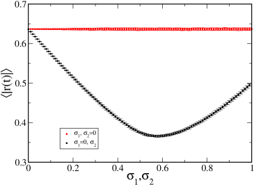
Figure 4: Average absolute value of the RoI, $r(t)$, eq. 16, for phase noise (red, top line) and for amplitude noise (black, bottom line).

Since the distribution of the RoI is independent of the noise level $\sigma_{1}$ for phase noise, it is expected that the average absolute RoI, Fig. 4, is constant with respect to $\sigma_{1}$ in the RoI. This, as we have explained, is not the case for the noise level $\sigma_{2}$ for amplitude noise, where the average absolute RoI is varying with respect to $\sigma_{2}$ in the RoI. For $\sigma_{1}=0$ and $\sigma_{2}=0$, the average absolute value of the RoI are equal. Roughly, the average absolute value of the RoI with amplitude noise decreases for $\sigma_{2}<0.6$ and it increases for $\sigma_{2}\geq 0.6$. This matches with the observations for the probability distributions: there, for $\sigma_{2}=0.5$, the values are concentrated around $r(t)=0$, leading to smaller $\left\langle\left|r(t)\right|\right\rangle$, and for $\sigma_{2}=0.1$ and $\sigma_{2}=0.9$, the values are less concentrated around $r(t)=0$, leading to larger $\left\langle\left|r(t)\right|\right\rangle$.

The average absolute RoI is of importance because its known from multiplicative stochastic processes [Sornette-Cont97, NavarroEtAl07], that for a constant investment $q(t)=q_{0}$ the better performing constant strategies are the ones that invest the least possible amount. In our model, the agents are forced to invest the minimum amount of $q_{min}=0.1$. Since $q(t)$ is multiplied with $r(t)$ in eq. 1, the change in average absolute value of $r(t)$ has an impact similar to the change in $q_{0}$ seen in the multiplicative stochastic processes [NavarroEtAl07] studied. This leads to changes in performance that are not necessarily related with the performance of agents, and should be taken into account when interpreting the results.

(a)                                                     (b)

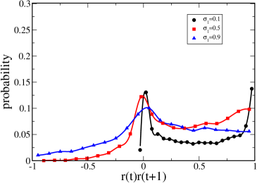
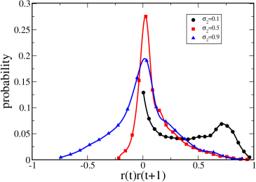
Figure 5: Distribution of the correlations of the RoI in time, $r(t)$, eq. 16, for: (a) phase noise with $\sigma_{1}=\{0.1,0.5,0.9\}$ and (b) amplitude noise with $\sigma_{2}=\{0.1,0.5,0.9\}$.

The correlation between the sign of two consecutive returns shows whether it is possible to draw conclusions from the sign of $r(t)$ on the sign of $r(t+1)$. In Fig. 5 we show the distribution of the correlations of the RoI with respect to two consecutive returns, $r(t)r(t+1)$. We can clearly see that for low levels of noise there is bigger correlation between consecutive values. As the noise increases this correlation diminishes until, finally, for high levels of noise, the returns are completely uncorrelated.

Most of the algorithms studied are sensitive to correlations in consecutive RoI with the same sign. We notice that between the returns with phase noise and amplitude noise, correlations do not vary exactly in the same manner with noise. In particular, it can clearly be seen that for $\sigma_{1,2}=0.5$ the amplitude noise has still more correlation than the phase noise. This difference can account for some discrepancies seen between the performance of the agents for the two types of market return functions.

5 Optimal Parameter Adjustment

In the previous sections, we have defined several different strategies that can be applied by agents to determine when to invest which amount of money. In the next section, we want to compare their performance in a periodic environment. However, in order to make this comparison meaningful, we have to ensure that we have adjusted the different parameters of the strategies properly. Only if the strategies perform at their optimum, they can really be compared.

The procedure that we apply to adjust the optimal parameters is straightforward: we compare the performance – averaged over $10^{5}$ periods – of each of the algorithms for a range of possible parameters and then choose the optimal one. At this point, it remains to define the notion of optimality: we have already defined that we measure the performance of agents as the average of their budget growth over a certain number of time steps. The optimal strategy is the strategy that performs better than all the other strategies, i.e. the strategy that, on average, leads to the greatest budget growth. Of course, for the measurement, each agent has to be provided with enough time to gather the information necessary for the proper calibration of the algorithm that it applies.

For the MA, MLS, and IUR strategies, there is only one parameter that requires adjustment: either the memory size $M$ (in the case of MA and MLS) or the step size $\gamma$ (in the case of IUR). This implies that for these strategies, it is possible to choose the optimal value of the parameter by comparing the average budget $\left\langle x(t)\right\rangle$ for several possible values of the parameter, and then take the one which gives the best results. For MA and MLS, we have considered memory sizes $M\in[1,50]$ and for IUR, we have considered step sizes $\gamma\in[0,1]$.

For the GA strategy, there are, however, several parameters which require adjustment: the population size, $C$, the crossover probability, $p_{c}$, the mutation probability, $p_{m}$, and the elitism size, $s$. Consequently, the process of finding the optimal combination of values for the parameters is not as trivial as for the other strategies. The +CARPS (Multiagent System for Configuring Algorithms in Real Problem Solving) tool [Monett04a, Monett04b] was used during this step. This application uses autonomous, distributed, cooperative agents that search for solutions to a configuration problem, thereby fine-tuning the meta-heuristic’s parameters. The agents in +CARPS apply a Random Restart Hill-Climbing approach and they exchange their so-far best solutions to the problem in the process. The intervals of definition, i.e. the intervals in which the most acceptable GA configurations should lie, were set as follows: $C\in\{50,100,200,500,1000\}$, $p_{c}\in\left[0.0,1.0\right]$, $p_{m}\in\left[0.0,1.0\right]$, and $s\in\left[0.0,0.5\right]$,

Table 1: Optimal Strategy Parameters

Algorithm	Parameters
MA	$M=5$ (risk-seeking), $M=2$ (risk-avoiding)
MLS	$M=25$ (both risk-seeking and risk-avoiding)
IUR	$\gamma=0.5$ (both risk-seeking and risk-avoiding)
GA	$C=1000$, $p_{c}=0.7$, $p_{m}=0.01$, $s=0.3$

Table 1 shows the optimal parameters that we choose for the comparison of the different strategies. Of course, the optimal parameters usually are not the same for different types and levels of noise or for risk-seeking and risk-avoiding behaviour, so at times, a compromise between several alternative values for different situations had to be found.

6 Results

In this section, we compare all strategies presented in this article for RoI with periodicity $T=100$ and different noise levels for both phase and amplitude noise. In our comparison, we consider a set of agents, each one using one of the following strategies: Q0 eq. (2), MA eq. (3), MLS eq. (6), IUR eq. (11), and GA eq. (15). Note that periodic returns with a periodicity changing over time are invested recently as well.[navarro-barrientos08]

In our comparison, we make two assumptions: first, all agents receive the same RoI at a particular time, i.e. the fact that some agents win or loose more than others is influenced only by their different strategies to determine the correct risk-propensity value; second, all agents use the optimal parameter values of their respective strategies. Let us state again that only the past and current values of $r(t)$ are known to the agents; they do not know the dynamics governing future values of $r(t)$.

We perform $N=100$ trials of the same experiment, i.e. RoI with same parameters, where at each end of a cycle of the RoI, i.e. for all $t$ such that $t{}\bmod{}T\equiv 0$, an average budget is obtained for each agent over the 100 trials. This is done for a large number of time steps, i.e. $t=10^{5}$. We vary the amplitude noise values, $\sigma_{2}\in(0,1)$, while leaving the phase noise value constant, $\sigma_{1}=0$, and we vary the phase noise values, $\sigma_{1}\in(0,1)$, while leaving the amplitude noise value constant, $\sigma_{2}=0$. For the simulations which distinguish between a risk-seeking and a risk-avoiding action upon a prediction of the RoI, we compute the average budget for both approaches. This gives us four variants of the simulations: amplitude noise/risk seeking, phase noise/risk seeking, amplitude noise/risk avoiding, and phase noise/risk avoiding.

6.1 Comparison

Fig. 6 shows the result of the simulations by plotting the average budget resulting from the different strategies against the noise level for each of the four variants of the simulations (amplitude noise/risk seeking in (a), phase noise/risk seeking in (b), amplitude noise/risk avoiding in (c), and phase noise/risk avoiding in (d)).

(a)                                                        (b)

(c)                                                        (d)

Figure 6: Average budget over $N=100$ trials, for agents using strategies Q0, MA, MLS, GA, IUR and SW (square wave, to be introduced in section 6.2), over $t=10^{5}$ time steps. Agents use optimal parameter values for RoI with periodicity, $T=100$, and different noise levels: (a) different amplitude noise values, $\sigma_{2}\in(0,1)$, and no phase noise, $\sigma_{1}=0$ with a risk-seeking strategy; (b) different phase noise values, $\sigma_{1}\in(0,1)$, and no amplitude noise, $\sigma_{2}=0$ with a risk-seeking strategy; (c) different amplitude noise values, $\sigma_{2}\in(0,1)$, and no phase noise, $\sigma_{1}=0$ with a risk-avoiding strategy, and (d) different phase noise values, $\sigma_{1}\in(0,1)$, and no amplitude noise, $\sigma_{2}=0$ with a risk-avoiding strategy.

For all variants of the simulations, the constant-risk strategy is the worst strategy. The constant-risk strategy always puts a constant proportion of the budget at stake. This money is won when the return is positive, but also lost when the return is negative; even though $\left\langle\left|r(t)\right|\right\rangle=0$, this leads to a loss in budget over time, as this is a well known property for multiplicative stochastic processes.

Furthermore, for all strategies, the average budget decreases with increasing noise. That is the expected behaviour: with increasing noise, the accuracy of the predictions made by the agents decreases, and thus they cannot necessarily chose the appropriate risk propensity in the action.

There are no significant crossovers of the performance of different strategies. In general, this implies that if a strategy $s_{1}$ performs better than a strategy $s_{2}$ for a given noise level $\sigma_{a}$ (either on the phase or on the amplitude), $s_{1}$ can be expected to perform better than $s_{2}$ for a different noise level $\sigma_{b}$. Consequently, the choice of strategy is independent of the noise in the return – a good strategy is a good strategy for all noise levels, and a bad strategy is a bad strategy for all noise levels, too. However, for low noise levels, the GA is slightly outperformed by the other strategies – this is due to the intrinsic stochastic nature of the algorithm; for the same reason, this algorithm performs better for high noise levels. Note that the experiments in this simulations are done for $t=10^{5}$ time steps, which corresponds also to the learning phase for the GA.

For phase noise, the average budget obtained is roughly comparable to that for amplitude noise, although the differences between strategies are greater for phase noise than for amplitude noise.

From the range of strategies employed, the simple strategies (MA, MLS, IUR) were almost always outperformed by the complex one (GA). Other researchers [Gode-Sunder93, Daniels-Farmer03] have shown that this needs not necessarily be the case.

6.2 Optimal Strategy

As a consequence of the comparison it is logical to investigate what would be the optimal strategy in the given scenario. Given the fact that the GA performs best of all the strategies, it makes sense to look at the $q(t)$ as chosen by the GA for $r(t)$ over time, in order to analyse why the GA performs so well. Fig. 7 plots the values of $r(t)$ and the corresponding $q(t)$ as chosen by the GA against time $t$ for different noises and from different times $t_{n}$ on. From the graph, it is visible that the behaviour of the GA resembles a square wave function which is a type of a ramp-rectangle function.

(a)                                                       (b)

(c)                                                       (d)

Figure 7: Values of the return $r(t)$ and the risk propensity $q(t)$ as chosen by the GA for RoI with different types of noise and for different times during the simulation: (a) amplitude noise, $\sigma_{1}=0,\sigma_{2}=0.5$, $t_{n}\approx 10,000$, (b) amplitude noise, $\sigma_{1}=0,\sigma_{2}=0.5$, $t_{n}\approx 100,000$, (c) phase noise, $\sigma_{1}=0.5,\sigma_{2}=0$, $t_{n}\approx 10,000$, (d) phase noise, $\sigma_{1}=0.5,\sigma_{2}=0$, $t_{n}\approx 100,000$.

The ramp-rectangle (RR) function maps RoI that are uncertain to increasing/decreasing risk-propensity values and RoI that are certainly positive or negative to a maximal or minimal risk-propensity value, respectively. The corresponding strategy is expressed as follows:

$$q(t+1)=\begin{cases}\left(\frac{q_{\mathrm{max}}-q_{\mathrm{min}}}{h_{1}}\right)\hat{t}+q_{\mathrm{min}}&\textrm{if $\hat{t}\in(0,h_{1})$}\\ q_{\mathrm{max}}&\textrm{if $\hat{t}\in[h_{1},h_{2}]$}\\ \left(\frac{q_{\mathrm{max}}-q_{\mathrm{min}}}{h_{2}-h_{3}}\right)(\hat{t}-h_{2})+q_{\mathrm{max}}&\textrm{if $\hat{t}\in(h_{2},h_{3})$}\\ q_{\mathrm{min}}&\textrm{if $\hat{t}\in[h_{3},h_{4}]$}\end{cases}$$ (18)

In this function, $h_{1}$ ($h_{3}$) sets the transition from an increasing (decreasing) ramp function to a rectangle function and $h_{2}$($h_{4}$) sets the transition from a rectangle function to a decreasing (increasing) ramp function. Moreover, for each time step, $t$, the following congruence is used: $\hat{t}\equiv t\bmod h_{4}$; this maps each time step $t\in(0,\infty)$ to a time step in the ramp-rectangle function, $\hat{t}\in(0,h_{4})$.

Furthermore, we assume that the differences between time steps when an agent increases and decreases its risk propensity values are symmetric. This means that the time difference $\triangle h$ between when the ramp function starts and stops to increase or decrease can be expressed as follows:

$$\triangle h=h_{1}=h_{3}-h_{2}$$ (19)

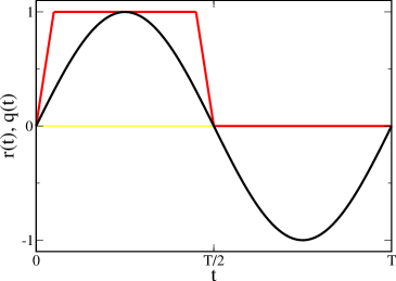
which for $\triangle h=1$, means that agents use a Square Wave (SW) strategy. We are particularly interested in this case of the ramp-rectangle function: it implies that an agent invests $q_{max}$ for time steps $\hat{t}\in(0,T/2)$, and invests $q_{min}$ for time steps $\hat{t}\in[T/2,T]$. This is the optimal strategy.

The GA approaches the optimal strategy: for all different noises, the risk propensity $q(t)$ chosen by the GA approximates the one that would have been chosen by SW. Considering that the GA does not have an ‘a priori’-behaviour defined, it is interesting to realise that it finds the optimal strategy – investing the maximum when, at a particular time $t$ in the period, the probability of winning is higher than loosing and vice versa – on its own.

Fig. 7 illustrates this behaviour. It plots the values of $r(t)$ and the corresponding $q(t)$ as chosen by the genetic algorithm against time $t$ for different noises and from different times $t_{n}$ on. From this, it is clearly visible that the behaviour of the GA is very similar to the behaviour of the SW, which is the optimal strategy. Comparing fig. 7 (a) with (b) and fig. 7 (c) with (d), i.e. the same scenario, but at different times $t_{n1}=10,000$ and $t_{n2}=100,000$, one can see that the $q(t)$ chosen by the GA approach the ones chosen by the SW more closely as time goes on – i.e., as the GA has more time to evolve. Additionally, from the simulation results, it can be observed the approximation of the SW by the GA is closer for low levels of noise than for high levels of noise. This is the expected behaviour.

6.3 “Everything on Red”

Furthermore, from the plots, we can observe that for low levels of noise, the risk-seeking behaviour clearly outperforms the risk-avoiding behaviour: always investing the maximum when a positive return is expected and investing the minimum when a negative return is expected outperforms investing a quantity proportional to the expected return. This may seem counter-intuitive – humans would probably choose not to invest their complete budget when they know that there is a certain probability to lose it.

However, this behaviour is explained as follows: consider $r(t)$ to be periodic with a period of $T$ and, for the moment, assume that there is no noise, i.e. $\sigma_{1}=0$ as well as $\sigma_{2}=0$. Then, the optimal strategy would be to invest the complete budget or $q_{max}$ during $[0,T/2)$ and to invest nothing or $q_{min}$ during $[T/2,T)$. This is because it is certain – we assumed that there is no noise – that during the first half of the period, $[0,T/2)$, the value of $r(t)$ will be positive and during the second half of the period, $[T/2,T)$, the value of $r(t)$ will be negative. No matter what the precise values of $r(t)$ are, once they are positive, this leads to a gain, and thus $q(t)$ should be as large as possible to maximise the gain; conversely, once the values of $r(t)$ are negative, this leads to a loss, and thus $q(t)$ should be as small as possible or zero to minimise the loss. In other words, for determining $q(t)$, not the quantity of the expected return matters, but whether the probability of the expected return being positive is greater than the probability of the expected return being negative. This explains why the risk-seeking behaviour outperforms the risk-avoiding behaviour for periodic returns with no noise. The behaviour of this strategy is shown in Fig. 8 (a).

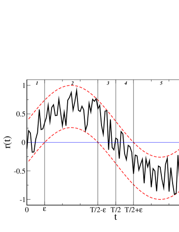
For periodic returns with noise, i.e., $\sigma_{1}\neq 0$ or $\sigma_{2}\neq 0$, the situation is quite similar. Depending on the values of $\sigma_{1}$ and $\sigma_{2}$, there will be two intervals $[0+\epsilon,(T/2)-\epsilon)$ and $[(T/2)+\epsilon,T-\epsilon)$ such that during $[0+\epsilon,(T/2)-\epsilon)$, the value of $r(t)$ will – on average – be positive and such that during $[(T/2)+\epsilon,T-\epsilon)$, the value of $r(t)$ will – on average – be negative, see Fig. 8 (a). In these intervals, the optimal strategy would again be to invest the complete budget or $q_{max}$ and to invest nothing or $q_{min}$, respectively. The value of $\epsilon$, of course, depends on $\sigma_{1}$ and $\sigma_{2}$, i.e. the more noise, the greater $\epsilon$. Now, what still has to be considered are the intervals $[0,0+\epsilon)$, $[(T/2)-\epsilon,(T/2)+\epsilon)$, and $[T-\epsilon,T)$. Because of the noise, it is not possible to determine the exact sign of $r(t)$ during these intervals.

(a)                                                     (b)

Figure 8: Intervals of certainty and uncertainty: (a) shows $r(t)$ with no noise and the corresponding $q(t)$ of the square wave (SW) strategy plotted against $t$ and (b) shows $r(t)$ with noise and the different intervals for which different conclusions about the sign of the return can be drawn: (2) and (5) are the intervals in which the sign of $r(t)$ is certain to be positive or negative, respectively, and (1), (3), (4), and (6) are the intervals in which the the sign of $r(t)$ is uncertain.

However, it still is possible to say that – on average – the probability of $r(t)$ being positive is greater than the probability of $r(t)$ being negative during $[0,0+\epsilon)$ and $[(T/2)-\epsilon,T/2)$ and the probability of $r(t)$ being negative is greater than the probability of $r(t)$ being positive during $[T/2,(T/2)+\epsilon)$ and $[T-\epsilon,T)$. Consequently, it makes sense to invest during $[0,0+\epsilon)$ and $[(T/2)-\epsilon,T/2)$ and not to invest during $[T/2,(T/2)+\epsilon)$ and $[T-\epsilon,T)$.

With such behaviour, there will, however, be the situation that an agent invests the complete budget, but the return is negative. In this type of situation, $\left|r(t)\right|$ depends on $\sigma_{1}$ and $\sigma_{2}$: for small $\sigma_{1}$ and $\sigma_{2}$, it will be small, too. Consequently, for low levels of noise, the product of $q(t)r(t)$ would be a small value, which signifies, for $r(t)<0$, a small loss, and for $r(t)>0$, a small gain. Thus, even for $q(t)=1$, the loss is bound to a proportion of the budget corresponding to the value of $r(t)$. This explains why the risk-seeking behaviour outperforms the risk-avoiding behaviour for low levels of noise. For high levels of noise, the product of $q(t)r(t)$ needs not necessarily be a small value, which potentially signifies, for $r(t)<0$, a large loss, and for $r(t)>0$, a large gain. Thus, an agent could potentially loose a significant amount of its budget if it invests the complete budget; this is the reason why, for high levels of noise, the risk-avoiding behaviour outperforms the risk-seeking behaviour.

This also provides a straightforward explanation why different algorithms using the same rule to determine $q(t)$ perform differently. Even though the best strategy is to still invest the maximum when there is a slightly better probability that $r(t)>0$ than that $r(t)\leq 0$, the algorithms fail to predict the exact probabilities of $r(t)>0$ and of $r(t)\leq 0$ with good enough accuracy to determine how to properly invest. In other words, the performance of the action depends on the accuracy of the prediction; if the accuracy of the prediction is high, then the performance of the action is good, and if the accuracy of the prediction is low, then the performance of the action is bad, too. The GA does not exhibit this prediction-action behaviour and it is able to adjust better than the other strategies.

7 Discussion and Conclusions

In this paper, we have presented a number of strategies that can be applied by agents in an investment market scenario with periodic returns and different types and levels of noise. We have compared their performance – the respective average budget growth over a certain number of time steps – and analysed the results. We have made three main observations:

1. The type of noise – whether the RoI has phase or amplitude noise – does not have a significant influence on the performance of the algorithms, while the level of noise certainly does – for increasing noise, we observe decreasing performance.

2. The GA performs best of all strategies for almost all scenarios; it discovers a strategy which resembles a square wave strategy and which follows the principle of always investing the complete budget or the maximum amount possible when the expected return is positive and not investing anything or the least amount possible when the expected return is negative.

3. The best rule for investment is the risk-seeking behaviour of always putting the complete budget in an investment; this behaviour clearly outperforms a risk-avoiding behaviour which humans would probably apply intuitively: whilst it may seem intuitive to a human to invest an amount proportional to the expected return, this is not the approach which yields the greatest budget growth over time.

Consequently, returning to our original goal to find an answer to the question of to which extent the internal complexity of agents influences their overall performance, we can state that, in our simple scenario, the agents with a complex architecture outperform the agents with a simple architecture.

Although, with respect to the question above, the major focus on this paper is more related to issues of computer science, one may also ask for the application of the results in an economic context, in particular to financial markets. Surely, our paper can be seen as a computational experiment on the performance of different trading strategies in face of noisy market returns. In this context, the agent in our model may have two possible preferences: liquidity preference [tobin58] and speculative preference. I.e. based on the previous returns the agent has a preference to keep cash or to invest in the market, respectively - which is modeled by the risk-seeking and risk-avoiding behavior.

Apart from this, our model allows only a limited interpretation in the context of financial markets, because a number of important features in these markets are not covered or are even explicitely excluded, for the sake of a controlled simulation setup:

Heterogeneity:

Agents in our model are homogenous with respect to the strategy employed, i.e. there is no variability in their individual strategies.[kirman05] In this respect, the model is basically a “representative agent model”, which takes into account only the limited information of the previous $r(t)$. More elaborated strategies, where agents are assumed to be fundamentalist or chartists [day90, farmer00price, follmer05] are also not considered here.

Interaction:

Agents in our model do not interact with other agents. They rather “learn” the dynamics of the market return, in order to predict it more accurately. Important collective interactions in financial markets, such as herding behavior, is neglected here, as well as interactions between (heterogeneous) trading strategies [follmer05]. This implies the absence of emergent properties in our model, as heterogeneity and interaction are indeed basic premises for the existence of emergent properties in financial markets.

Feedback:

Agents in our model have no effect upon the market, and consequently the price of an asset and the return on investment are treated as exogenous variables. This is equivalent to the ’atomistic market’ assumption. Our model also neglects the collective impact of all agents on the price and the return of an asset. Other feedbacks on the market, such as agent’s expectations about the market dynamics itself, are also not explicitely modeled here. Some artificial market models consider an endogeneous approach, where the returns are generated by means of constant trading between heterogeneous agents [day90, farmer00price].

Microfoundation:

Our model is lacking an adequate economic microfoundation of the (representative) agent behaviour. The terms “risk-avoiding” and “risk-seeking” are used to denote the investment preference of the agent. However, since decisions are always taken based on just the expected return, the behaviour of the agent has to be classified as “risk neutral” – risk-adverse agents indeed account also for the “variance” of returns in their decisions. Recent literature in economics and finance presents a more realistic approach about behaviour toward risk. [hens06, Pindyck-Rubinfeld]

Multi-assets:

Agents in our model can only invest in one (risky) asset, whereas in financial markets multi-asset investments and portfolio strategies play the most crucial role. [elton03, markowitz91] Multi-asset optimal investment strategies for risky assets were already discussed 50 years ago, with an interesting relation to gambling [breiman60]. More recently, investment strategies to readjust portfolios [merton90] have been extended [maslov98] for a general distribution of return per capital. Similar to our model, these contributions consider exogeneous returns which are drawn from a probability distribution or are modeled by a stochastic processes.

Acknowledgements

We thank Dagmar Monett Díaz for her help in finding the optimal parameters for the genetic algorithm applied in this paper using the +CARPS tool and shown in Table 1. We furthermore thank João F. M. Rodrigues, Mauro Napoletano and Robert Mach for valuable comments and discussions, and the latter one for his help in obtaining the data and creating the plots for Figure 1.