A generalisation of the mass-sheet degeneracy producing ring-like artefacts in the lens mass distribution

Abstract

The inversion of a gravitational lens system is, as is well known, plagued by the so-called mass-sheet degeneracy: one can always rescale the density distribution of the lens and add a constant-density mass-sheet such that the, also properly rescaled, source plane is projected onto the same observed images. For strong lensing systems, it is often claimed that this degeneracy is broken as soon as two or more sources at different redshifts are available. This is definitely true in the strict sense that it is then impossible to add a constant-density mass-sheet to the rescaled density of the lens without affecting the resulting images. However, often one can easily construct a more general mass distribution – instead of a constant-density sheet of mass – which gives rise to the same effect: a uniform scaling of the sources involved without affecting the observed images. We show that this can be achieved by adding one or more circularly symmetric mass distributions, each with its own center of symmetry, to the rescaled mass distribution of the original lens. As it uses circularly symmetric distributions, this procedure can lead to the introduction of ring shaped features in the mass distribution of the lens. In this paper, we show explicitly how degenerate inversions for a given strong lensing system can be constructed. It then becomes clear that many constraints are needed to effectively break this degeneracy.

1 Introduction

Being an ill-posed problem, it is not surprising that gravitational lens inversion is plagued by degeneracies. Several classes of degeneracies were first identified by Gorenstein et al. (1988) and were later reinterpreted by Saha (2000) in terms of changes in the arrival-time surface. Of these, the most widely known degeneracy is usually called the mass-sheet degeneracy, although recently the more correct name of steepness degeneracy has been suggested (Saha & Williams, 2006). This degeneracy was first mentioned in the context of the strong lensing system Q0957+561 (Falco et al., 1985), but has also been studied in weak lensing systems (e.g. Schneider & Seitz (1995)) and even in the context of microlensing (Paczynski, 1986).

In strong lensing systems, it is often claimed that the presence of two sources at different redshifts suffices to break the mass-sheet degeneracy (e.g. Abdelsalam et al. (1998)). While it is definitely true that a constant-density mass-sheet can no longer be used to construct degenerate solutions in such a case, we show in this paper how a more general mass distribution, to be added to the original lens mass distribution, can be constructed which gives rise to a similar type of degenerate solutions. In particular, the alternative name of steepness degeneracy is still applicable since the construction of degenerate solutions still requires the original mass distribution to be rescaled. Although the method described below is quite straightforward, the authors, having performed a thorough literature study, are not aware of this result being published before.

In section 2 the necessary equations from the gravitational lensing formalism will be reviewed. These equations will be used to derive the mass-sheet degeneracy in section 3 and to explain the extension to multiple redshifts in section 4. Finally, in section 5, the results and their implications are discussed.

2 Lensing formalism

We shall briefly review the necessary equations related to the gravitational lensing formalism. The interested reader is referred to Schneider et al. (1992) for a thorough review of gravitational lensing theory.

In the thin lens approximation, the gravitational lens effect is essentially a mapping of the source plane ($\beta$-space) onto the image plane ($\theta$-space), described by the lens equation:

$$\mbox{\boldmath$\beta$}(\mbox{\boldmath$\theta$})=\mbox{\boldmath$\theta$}-\frac{D_{\rm ds}}{D_{\rm s}}\mbox{\boldmath$\hat{\alpha}$}(\mbox{\boldmath$\theta$})\mathrm{.}$$ (1)

Here, $\mbox{\boldmath$\hat{\alpha}$}(\mbox{\boldmath$\theta$})$ describes the instantaneous deflection of a light ray that punctures the lens plane at the position $\theta$, and depends linearly on the two-dimensional projected surface mass density $\Sigma(\mbox{\boldmath$\theta$})$ of the lens.

For a circularly symmetric projected mass density centered on the origin, the defection angle reduces to:

$$\mbox{\boldmath$\hat{\alpha}$}(\mbox{\boldmath$\theta$})=\frac{4GM(\theta)}{c^{2}D_{\rm d}\theta^{2}}\mbox{\boldmath$\theta$}\mathrm{,}$$ (2)

in which $M(\theta)$ is the total mass within a radius $\theta$. The geometry of the situation is described by the angular diameter distances $D_{\rm d}$, $D_{\rm ds}$ and $D_{\rm s}$. As a result, for a circularly symmetric projected mass distribution, only the total mass inside a specific radius contributes to the deflection of light rays.

Figure 1: Left panel: original sources used to illustrate the construction of degenerate solutions. The source surrounded by a box is placed at redshift $z_{1}=1.2$, the second source is at $z_{2}=1.8$. The caustics created by the non-singular isothermal ellipse placed at $z=0.5$ are also visible. The solid line corresponds to $z_{1}=1.2$, the dotted line to $z_{2}=1.8$. Right panel: images of the two sources used to illustrate the construction of degenerate solutions. The critical lines are also shown.

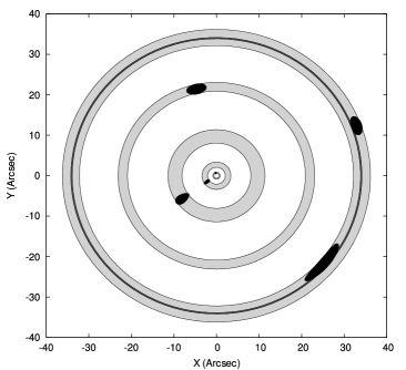
Figure 2: Left panel: the annuli in which the images reside, as seen from the origin of the coordinate system, are displayed as grey rings. The darker ring indicates the region in which the annuli of the outer images overlap. Because of this overlap, no suitable mass density can be constructed (see text). Right panel: similar to the left panel, but now the annuli are centered on $(0,-5)$. This center can be used in the construction of a degenerate solution since there are no longer overlapping annuli.

3 The mass-sheet degeneracy

Let us first consider a strong lensing system with images coming from a single source. A uniform sheet of mass with density $\Sigma_{\rm s}$ produces a deflection described by

$$\mbox{\boldmath$\hat{\alpha}$}_{\rm s}(\mbox{\boldmath$\theta$})=\frac{D_{\rm s}}{D_{\rm ds}}\frac{\Sigma_{\rm s}}{\Sigma_{\rm cr}}\mbox{\boldmath$\theta$}\mathrm{,}$$ (3)

in which the critical mass density for the current geometry is defined as follows:

$$\Sigma_{\rm cr}=\frac{c^{2}}{4\pi GD_{\rm d}}\frac{D_{\rm s}}{D_{\rm ds}}\mathrm{.}$$ (4)

Note that $\Sigma_{\rm cr}$ depends on the redshift of the source via the angular diameter distances $D_{\rm s}$ and $D_{\rm ds}$. Let $\Sigma_{0}(\mbox{\boldmath$\theta$})$ be a mass distribution that is compatible with the observed images. This means that the corresponding lens equation

$$\mbox{\boldmath$\beta$}_{0}(\mbox{\boldmath$\theta$})=\mbox{\boldmath$\theta$}-\frac{D_{\rm ds}}{D_{\rm s}}\mbox{\boldmath$\hat{\alpha}$}_{0}(\mbox{\boldmath$\theta$})$$ (5)

projects the images onto the source plane in such a way that they overlap exactly. Without further constraints, this immediately yields an infinite number of alternative solutions. Indeed, if the mass distribution is replaced by

$$\Sigma_{1}(\mbox{\boldmath$\theta$})=\lambda\Sigma_{0}(\mbox{\boldmath$\theta$})+(1-\lambda)\Sigma_{\rm cr}\mathrm{,}$$ (6)

the new lens equation becomes

$$\mbox{\boldmath$\beta$}_{1}(\mbox{\boldmath$\theta$})=\mbox{\boldmath$\theta$}-\lambda\frac{D_{\rm ds}}{D_{\rm s}}\mbox{\boldmath$\hat{\alpha}$}_{0}(\mbox{\boldmath$\theta$})-(1-\lambda)\frac{D_{\rm ds}}{D_{\rm s}}\mbox{\boldmath$\hat{\alpha}$}_{\rm s}(\mbox{\boldmath$\theta$})=\lambda\mbox{\boldmath$\beta$}_{0}(\mbox{\boldmath$\theta$})\mathrm{.}$$ (7)

The transformation (6) describes the so-called mass-sheet degeneracy and simply rescales the source plane by the factor $\lambda$, producing an equally acceptable source reconstruction. Note that merely adding a mass-sheet is not sufficient; one also needs to rescale the original mass distribution by the same factor $\lambda$, which justifies the alternative name of steepness degeneracy. The density of the mass-sheet has to be precisely the critical mass density for this to work. For this reason, a mass-sheet cannot be used when there are sources at different redshifts, since these would require different critical densities.

4 Extension to multiple redshifts

An infinite sheet of mass, however, is not the only mass distribution which can be used to produce degenerate solutions. If the mass density is circularly symmetric and equal to $\Sigma_{\rm cr}$ in an area large enough to encompass all the images, the same source scaling effect will arise, thanks to equation (2). The center of symmetry of such a distribution determines the center of the scaling (which is the origin of the coordinate system in case of an infinite sheet). This way, the mass-sheet degeneracy is easily transformed into a mass-disk degeneracy. In fact, the added mass density need not be constant inside such a disk to produce the same effect. As long as the total mass inside each image point is the same as for the mass-disk, equation (2) ensures that the distribution can be used to construct a degenerate solution as well. This constraint automatically implies a density equal to $\Sigma_{\rm cr}$ inside the annuli in which the images reside, but otherwise allows a lot of freedom.

This freedom allows us to construct a mass distribution which, when added to a scaled version of an existing solution for the lens mass density, is equally compatible with the observed images, but which will rescale the sources. The effect is therefore very similar to that of the mass-sheet degeneracy, but this degeneracy is not necessarily broken by the presence of additional images of sources at different redshifts.

To illustrate the procedure, consider the two sources and their respective images in Fig. 1. The two sources are placed at redshifts $z_{1}=1.2$ and $z_{2}=1.8$ and the images are created by a non-singular isothermal ellipse at $z=0.5$. This non-singular isothermal ellipse then provides us with the initial mass density $\Sigma_{0}(\mbox{\boldmath$\theta$})$. A flat cosmological model with $\Omega_{\rm m}=0.27$, $\Omega_{\Lambda}=0.73$ and $H_{0}=70\,\textrm{km}\,\textrm{s}^{-1}\,\textrm{Mpc}^{-1}$ was used to calculate the necessary angular diameter distances.

The circularly symmetric mass density $\Sigma_{\rm gen}(\theta)$ and corresponding $M_{\rm gen}(\theta)$ that we shall construct, must have the same effect as a mass-sheet for both sources. This mass density will serve as the generator of the transformation which creates a degenerate solution $\Sigma_{1}(\mbox{\boldmath$\theta$})$ from an existing solution $\Sigma_{0}(\mbox{\boldmath$\theta$})$. The procedure is very similar to the mass-sheet case:

$$\Sigma_{1}(\mbox{\boldmath$\theta$})=\lambda\Sigma_{0}(\mbox{\boldmath$\theta$})+(1-\lambda)\Sigma_{\rm gen}(|\mbox{\boldmath$\theta$}-\mbox{\boldmath$\theta$}_{\rm c}|)\mathrm{,}$$ (8)

in which $\mbox{\boldmath$\theta$}_{\rm c}$ is the center of symmetry of the generator. The mass distribution of the generator must satisfy constraints provided by the images: the mass enclosed by each image point must equal the mass of the corresponding constant-density mass-sheet. Therefore, if a specific image of a source at redshift $z$ lies in an annulus with inner radius $\theta_{\rm in}$ and outer radius $\theta_{\rm out}$, the constraint provided by said image is the following:

$$\forall\theta\in[\theta_{\rm in},\theta_{\rm out}]:M_{\rm gen}(\theta)=\pi D_{\rm d}^{2}\theta^{2}\Sigma_{\rm cr}(z)\mathrm{,}$$ (9)

in which the radii are measured with respect to the chosen center of symmetry $\mbox{\boldmath$\theta$}_{\rm c}$. Consequently, within such an annulus the mass density must equal the critical density for an image at redshift $z$ and in the region enclosed by the annulus, the mean density must equal the critical density. In the left panel of Fig. 2, we plot the annuli of the images, as seen from the center of the non-singular isothermal ellipse. Looking at the furthest image of each source, it is clear that no $\Sigma_{\rm gen}$ can be constructed. The mass density would have to be equal to $\Sigma_{\rm cr}(z_{1})$ inside the annulus of one image and $\Sigma_{\rm cr}(z_{2})$ inside the annulus of the other image. Since these regions overlap, as is indicated by the darker ring, this is impossible. However, if we take $(0,-5)$ as the center, there are no overlapping annuli as can be seen in the right panel of Fig. 2.

Figure 3: Left panel: the positions of the images of each source place constraints on the enclosed mass $M_{\rm gen}$ (thick lines on the mass profile). The regions in between can easily be interpolated. Right panel: the total mass profile in the left panel gives rise to the density profile $\Sigma_{\rm gen}$ shown here. The dotted lines indicate the critical mass densities for the two sources.

Figure 4: The profile of the degenerate solution (thick line) is compared to the profile of the original mass distribution, a non-singular isothermal ellipse. In this example, $\lambda=0.75$ was used.

Figure 5: Sources recreated by the degenerate solution (thick solid lines); the original sources are indicated by dotted lines. The direction of the scaling is clearly towards $(0,-5)$.

Figure 6: Left panel: sources and caustics predicted by a degenerate solution. Comparing with the left panel of Fig. 1 one sees that both sources and caustics are scaled versions of their original counterparts. Right panel: the reconstructed sources and caustics shown in the left panel predict the images and critical lines shown here. The same images as in the right panel of Fig. 1 can be seen and the critical lines still resemble the original ones.

Figure 7: Left panel: the degenerate solution which gives rise to the source and image planes shown in Fig. 6. Several ring-like features can be seen, the most prominent one being centered on $(-8,-8)$. Right panel: density profile as seen from $(-8,-8)$. Apart from the peak of the non-singular isothermal ellipse, one can clearly see a ring-like feature.

Once an appropriate center has been identified, the positions of the images of each source can be used to calculate parts of the total mass map $M_{\rm gen}(\theta)$, as specified by (9). In our example, these constraints are illustrated by thick black lines in Fig. 3 (left panel), when using $(0,-5)$ as the center of the distribution. The rest of the mass map can easily be interpolated, after which the full density profile of $\Sigma_{\rm gen}(\theta)$ can be derived. In the left panel of Fig. 3, a third degree polynomial was used to interpolate between the constrained regions. The resulting density profile is plotted in in the right panel of the same figure and the critical densities for the two sources are indicated with dotted lines. Note that although this particular example does not require negative densities, in general it is possible that this is indeed necessary. This need not be a problem, since the resulting mass distribution will be combined with the existing distribution $\Sigma_{0}(\mbox{\boldmath$\theta$})$ (the non-singular isothermal ellipse in this example) and may still yield an overall positive density profile. Still, placing a positivity constraint on the overall density profile may help to alleviate this degeneracy.

By construction, the procedure (8) has the same effect as the mass-sheet degeneracy: the observed images are identical but the reconstructed sources are scaled versions of the original ones while the density profile of the lens has become less steep. The resulting density profile for $\lambda=0.75$ can be seen in Fig. 5, in which the original profile is shown as well. Clearly, the central peak has become weaker while at larger radii a ring of excess density has been introduced. This figure illustrates nicely that the term steepness degeneracy still applies to this kind of degenerate solution. When the images of Fig. 1 are projected back onto their source planes using the new mass distribution $\Sigma_{1}$, the sources in Fig. 5 (solid lines) are retrieved. The fact that the images of a specific source overlap perfectly when projected onto the source plane proves that the constructed mass distribution is still compatible with the observed images and can therefore correctly be identified as a degenerate solution. Since each dimension is scaled by $\lambda=0.75$, the reconstructed sources are smaller than the original ones (dotted lines). The image also clearly shows that the direction of the scaling is towards $(0,-5)$, the center of the circularly symmetric $\Sigma_{\rm gen}$ which was constructed.

Of course, since the positions of the images are not affected, one is free to repeat the entire procedure using the newly acquired $\Sigma_{1}$ as the “original” solution. In general, if it is possible to create $N$ different circularly symmetric density distributions $\Sigma_{{\rm gen},i}$, each with another center of symmetry $\mbox{\boldmath$\theta$}_{{\rm c},i}$, it is easily derived that for any $\lambda$, the following mass distribution will still project the images back onto consistent sources:

$$\Sigma_{N}(\mbox{\boldmath$\theta$})=\lambda^{N}\Sigma_{0}(\mbox{\boldmath$\theta$})+(1-\lambda)\sum_{i=1}^{N}\lambda^{N-i}\Sigma_{{\rm gen},i}(|\mbox{\boldmath$\theta$}-\mbox{\boldmath$\theta$}_{{\rm c},i}|)\mathrm{.}$$ (10)

This way, the mass distribution which is added to $\Sigma_{0}$ need not possess circular symmetry anymore and its density profile can become much more complex. Equation (10) is important from a practical point of view: the target scale $\lambda^{N}$ can easily be reached by using $N$ generators, each producing only a very small effect. If a large number of suitable center positions can be found, this can severely reduce the amount of substructure introduced by the procedure.

An example of degenerate source and image planes obtained by using $N=100$ different $\Sigma_{{\rm gen},i}$ can be seen in Fig. 6. Each source is scaled by a factor $\lambda^{N}=0.75$ in each dimension; the caustics are scaled as well. The critical lines still show the same general structure. The mass distribution of the degenerate solution can be seen in Fig. 7 (left panel) and contains several ring-like structures, the most prominent one being centered on $(-8,-8)$. This can also be clearly seen when the density profile is calculated using $(-8,-8)$ as the center (right panel of Fig. 7). The first peak in this plot is due to the non-singular isothermal ellipse, the second one is caused by the ring-like substructure of the degenerate solution. Note that the ring is not caused by one particular generator, but is a combined effect.

As an aside, even when it is impossible to rescale the sources, it may still be possible to introduce ring-shaped features. One only needs a ring-shaped region without data points. A circularly symmetric distribution which is zero everywhere but which fluctuates in the ring-shaped region in such a way that the total mass inside the region is zero as well, can simply be added to the original, again thanks to equation (2). Doing so can obviously introduce a ring-like feature in the mass distribution of the lens.

5 Discussion and conclusion

In this article we have presented a straightforward extension of the mass-sheet degeneracy to multiple redshifts. Although there is no actual sheet of mass involved, the procedure and effect of the degeneracy are the same. In both cases, the existing mass distribution is rescaled and a component is added, leading to a rescaling of the sources. This justifies placing the degeneracy described above in the same category as the mass-sheet or steepness degeneracy. Although we illustrated the construction of degenerate solutions using a strong lensing example, it is clear that weak lensing studies can be affected as well. In particular, if weak lensing data alone leads to solutions prone to the mass-sheet degeneracy, it will not suffice to add strong lensing data of a single source to break the degeneracy if strong and weak lensing regions do not overlap. Otherwise, a similar construction as above is possible, using one critical density in the weak lensing region and another in the strong lensing region.

However, as was shown by Bradač et al. (2004), using weak lensing data it is in principle possible to break the mass-sheet degeneracy – including the extension described here – if individual source redshifts are available and if sources with a rather high distortion are included. Another way to break the degeneracy is to add information about the magnification, for example by using source number statistics (Broadhurst et al., 1995) or Type Ia supernovae observations (Holz, 2001). Additional information about stellar dynamics in the gravitational lens can also help to break the degeneracy (Koopmans, 2006). Since the mass-sheet degeneracy rescales the time delay surface, time delay measurements can be used to break it as well.

This degeneracy seems to explain what we observed during tests of our non-parametric inversion algorithm (Liesenborgs et al., 2007). Although an example using two sources was used to avoid the mass-sheet degeneracy, we found that our algorithm did not succeed in finding the correct source sizes. However, the general shape and features of the reconstructed mass map did resemble closely the true mass distribution, which was used to create the images that served as input for the inversion routine. It is now clear that images of two sources at different redshifts do not provide enough constraints to firmly establish the scale of these sources.

The procedure outlined above still allows much freedom in the interpolation scheme, and therefore in the precise shape of $\Sigma_{\rm gen}$. It is clear, however, that in general it will always be necessary to introduce substructure in $\Sigma_{\rm gen}$, which may lead to the presence of substructure in the new mass map. The presence of such substructure will limit the range in which the parameter $\lambda$ may lie: if too much substructure is introduced, additional images will be predicted and the created mass distribution will no longer be compatible with the observed situation. However, by using several versions of $\Sigma_{\rm gen}$, each with a different center of symmetry, the amount of substructure that needs to be introduced to obtain a specific scaling can be limited.

It is straightforward to extend the procedure to more than two sources, but at some point it will no longer be possible to construct such degenerate solutions. How many sources are needed will depend on a number of factors. The number of the images and their sizes play an important role, as this determines how easily their annuli will overlap and therefore how difficult it will be to find appropriate scaling centers. The precise redshifts of the sources will determine how much substructure needs to be introduced, since the redshifts will determine if the corresponding critical densities lie close to each other or differ a lot. If the latter is the case, automatically more substructure will need to be introduced, allowing only a limited range of $\lambda$ values to avoid the prediction of extra images.

Although at a first glance the mass-sheet or steepness degeneracy is easily broken, this article shows that it is in fact a lot more difficult to do so and a relatively large number of constraints may be needed. The examples above also suggest that circularly symmetric features should be distrusted, as they are easily introduced in degenerate solutions.

References

- Abdelsalam et al. (1998) Abdelsalam H. M., Saha P., Williams L. L. R., 1998, AJ, 116, 1541
- Bradač et al. (2004) Bradač M., Lombardi M., Schneider P., 2004, A&A, 424, 13
- Broadhurst et al. (1995) Broadhurst T. J., Taylor A. N., Peacock J. A., 1995, ApJ, 438, 49
- Falco et al. (1985) Falco E. E., Gorenstein M. V., Shapiro I. I., 1985, ApJ, 289, L1
- Gorenstein et al. (1988) Gorenstein M. V., Shapiro I. I., Falco E. E., 1988, ApJ, 327, 693
- Holz (2001) Holz D. E., 2001, ApJ, 556, L71
- Koopmans (2006) Koopmans L. V. E., 2006, in EAS Publications Series, Vol. 20, EAS Publications Series, Mamon G. A., Combes F., Deffayet C., Fort B., eds., pp. 161–166
- Liesenborgs et al. (2007) Liesenborgs J., De Rijcke S., Dejonghe H., Bekaert P., 2007, MNRAS, 380, 1729
- Paczynski (1986) Paczynski B., 1986, ApJ, 301, 503
- Saha (2000) Saha P., 2000, AJ, 120, 1654
- Saha & Williams (2006) Saha P., Williams L. L. R., 2006, ApJ, 653, 936
- Schneider et al. (1992) Schneider P., Ehlers J., Falco E. E., 1992, Gravitational Lenses. Springer-Verlag, Berlin
- Schneider & Seitz (1995) Schneider P., Seitz C., 1995, A&A, 294, 411