Orbifold construction of the modes
of the Poincaré dodecahedral space

Abstract

We provide a new construction of the modes of the Poincaré dodecahedral space $S^{3}/I^{*}$. The construction uses the Hopf map, Maxwell’s multipole vectors and orbifolds. In particular, the *235-orbifold serves as a parameter space for the modes of $S^{3}/I^{*}$, shedding new light on the geometrical significance of the dimension of each space of $k$-modes, as well as on the modes themselves.

Keywords: Poincaré dodecahedral space, spherical 3-manifold, eigenmodes of the Laplace operator, Hopf fibration, multipole vectors, orbifold

1 Introduction

Cosmological motivations [1] have inspired recent progress in understanding the eigenmodes of the spherical spaces $S^{3}/\Gamma^{*}$, i.e., the quotients of the three-sphere $S^{3}$ by a binary polyhedral group $\Gamma^{*}$. Such modes may be seen as the $\Gamma^{*}$-invariant solutions of the Helmoltz equation in the universal cover $S^{3}$. Their numeration and degeneracy were given by Ikeda [2]. Recent works [3, 4, 5] have provided various means to calculate them.

Here we give a new point of view, using the Hopf map, multipole vectors and orbifolds to construct the modes of $S^{3}/\Gamma^{*}$ and shed additional light on the geometrical significance of Ikeda’s formula. Section 2 reviews the Hopf map and uses it to lift eigenmodes from $S^{2}$ to $S^{3}$. Section 3 uses twist operators to extend the lifted modes to a full eigenbasis for $S^{3}$. Section 4 generalizes the preceding results from the modes of $S^{3}$ to the modes of a spherical space $S^{3}/\Gamma^{*}$, showing that the latter all come from the lifts of the those eigenmodes of $S^{2}$ that are invariant under the corresponding (non-binary) polyhedral group $\Gamma$. We then turn to a detailed study of the $\Gamma$-invariant modes of $S^{2}$. Section 5 recalls Maxwell’s multipole vector approach and uses it to associate each mode of $S^{2}/\Gamma$ to a $\Gamma$-invariant set of multipole directions. Restricting attention to the case that $\Gamma$ is the icosahedral group, Section 6 introduces the concept of an orbifold and re-interprets a $\Gamma$-invariant set of multipole directions as a (much smaller) set of points in the *235-orbifold, which serves as the parameter space. Section 7 pulls together the results of the preceding sections to summarize the construction of the modes of the Poincaré dodecahedral space and state the dimension of the mode space for each $k$.

2 From $S^{2}$ to $S^{3}$: lifting with the Hopf map

2.1 Spheres

We parameterize the circle $S^{1}$ as the set of points $\alpha\in\mathbb{C}$ of unit norm $\alpha\bar{\alpha}=1$. The relationship between the complex coordinate $\alpha$ and the usual Cartesian coordinates $(x,y)$ is the natural one: $\alpha=x+iy$.

We parameterize the 2-sphere $S^{2}$ as the set of points $(x,y,z)\in\mathbb{R}^{3}$ of unit norm $x^{2}+y^{2}+z^{2}=1$.

We parameterize the 3-sphere $S^{3}$ as the unit sphere in $\mathbb{C}^{2}$: the set of points $(\alpha,\beta)\in\mathbb{C}^{2}$ of unit norm $\alpha\bar{\alpha}+\beta\bar{\beta}=1$. Hereafter, we will always assume that this normalization relation holds. The relationship between the complex coordinates $(\alpha,\beta)$ and the usual Cartesian coordinates $(x,y,z,w)$ is the natural one: $\alpha=x+iy$ and $\beta=z+iw$.

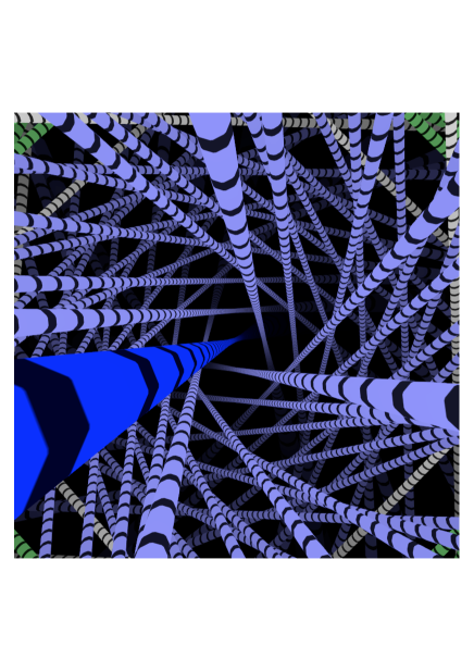
Figure 1: A computer generated view of the Clifford parallels in $S^{3}$

2.2 The Hopf fibration

In $S^{3}$, simultaneous rotation in the $\alpha$- and $\beta$-planes defines the Hopf flow $H_{t}:S^{3}\rightarrow S^{3}$,

$$H_{t}(\alpha,\beta)\equiv(\;e^{it}\alpha,\;e^{it}\beta\;).$$ (1)

The Hopf flow is homogeneous in the sense that it looks the same at all points. An orbit

$$\{\;(e^{it}\alpha,e^{it}\beta)\quad|\quad 0\leq t<2\pi\}.$$ (2)

is a great circle on $S^{3}$ called a Clifford parallel (Figure 1). Collectively the Clifford parallels comprise the Hopf fibration of $S^{3}$. The fibers carry Clifford’s name because William Kingdon Clifford (1845 – 1879) discovered them before Heinz Hopf (1894 – 1971) was born. However, while Clifford understood the fibration quite well, he did not, as far as we know, go on to consider the quotient map (Eqn. (3)).

As we walk along any given Clifford parallel $(e^{it}\alpha,e^{it}\beta)$, the ratio of its coordinates $\frac{e^{it}\alpha}{e^{it}\beta}$ remains a constant $\frac{\alpha}{\beta}$, independent of $t$. The ratio $\frac{\alpha}{\beta}$ labels uniquely each Clifford parallel, taking values in the extended complex numbers $\mathbb{C}\cup\{\infty\}$, where $\infty$ represents the ratio $\frac{\alpha}{\beta}=\frac{1}{0}$. The extended complex numbers may be visualized as a Riemann sphere, proving that the Clifford parallels are in one-to-one correspondence with the points of a topological 2-sphere $S$.

The Hopf map is defined as sending any point $(\alpha,\beta)$ of $S^{3}$ to the fiber its belong to, i.e., the point of $S$ labelled by $\frac{\alpha}{\beta}$. Composing with a natural map from $S$ to the unit 2-sphere $S^{2}$ gives an explicit formula for the Hopf map:

$$p:S^{3}\rightarrow S^{2}$$ (3)

$$(\alpha,\beta)\rightarrow p(\alpha,\beta)=(x,y,z)=\left(\;\alpha\bar{\beta}+\bar{\alpha}\beta,\;-i\;(\alpha\bar{\beta}-\bar{\alpha}\beta),\;\beta\bar{\beta}-\alpha\bar{\alpha}\;\right)$$ .

It is easy to check that $x^{2}+y^{2}+z^{2}=1$, confirming that the Hopf map $p$ sends $S^{3}$ to the the unit 2-sphere.

2.3 Lifts of functions

Any given function $f$ on $S^{2}$ lifts to a function $F$ on $S^{3}$ by composition with the Hopf map $p$ from Equation (3),

$$F:S^{3}\xrightarrow{\;p\;}S^{2}\xrightarrow{\;f\;}\mathbb{R}.$$ (4)

In other words, $F=p^{*}f$ is the pull-back of $f$ by $p$: explicitly,

$$F(\alpha,\beta)\equiv f(p(\alpha,\beta))=f\left(\alpha\bar{\beta}+\bar{\alpha}\beta,\;-i\;(\alpha\bar{\beta}-\bar{\alpha}\beta),\;\beta\bar{\beta}-\alpha\bar{\alpha}\right).$$ (5)

For example, the quadratic polynomial

$$f(x,y,z)=x^{2}-y^{2},$$ (6)

lifts to the quartic polynomial

$$F(\alpha,\beta) = (\alpha\bar{\beta}+\bar{\alpha}\beta)^{2}-(-i\;(\alpha\bar{\beta}-\bar{\alpha}\beta))^{2}$$ (7)

$$= 2(\alpha^{2}\bar{\beta}^{2}+\bar{\alpha}^{2}\beta^{2}).$$

Definition 2.3.1. We call a function $F:S^{3}\rightarrow\mathbb{R}$ vertical if it is constant along every Clifford parallel (Formula (2)).

For every function $f:S^{2}\rightarrow\mathbb{R}$, the construction of the lift $F(\alpha,\beta)=f(p(\alpha,\beta))$ guarantees that $F$ is vertical.

Proposition 2.3.2. The Hopf map lifts a polynomial $f:S^{2}\rightarrow\mathbb{R}$ of degree $\ell$ to a polynomial $F:S^{3}\rightarrow\mathbb{R}$ of degree $2\ell$.

Proof. The lifting formula (5) doubles the degree of any polynomial. $\blacksquare$

3 Eigenmodes

3.1 Basic definitions

Definition 3.1.1. An $\ell$-eigenmode is an eigenmode $f:S^{2}\rightarrow\mathbb{R}$ of the Laplacian, with eigenvalue $\lambda_{\ell}=\ell(\ell+1)$.

An $\ell$-eigenmode is a solution of the Helmholtz equation

$$\Delta_{S^{2}}f=\ell(\ell+1)f.$$ (8)

The index $\ell$ takes values in the set $\{0,1,2,\ldots\}$. For each $\ell$, the $\ell$-eigenmodes (which are the usual spherical harmonics) form a vector space $V^{\ell}$ of dimension $2\ell+1$.

Definition 3.1.2. A $k$-eigenmode is an eigenmode $F:S^{3}\rightarrow\mathbb{R}$ of the Laplacian with eigenvalue $\lambda_{k}=k(k+2)$.

A $k$-eigenmode is a solution of the Helmholtz equation

$$\Delta_{S^{3}}F=k(k+2)~{}F.$$ (9)

The index $k$ takes values in the set $\{0,1,2,\ldots\}$. For each $k$, the $k$-eigenmodes form a vector space $V^{k}$ of dimension $(k+1)^{2}$.

3.2 Eigenmodes of $S^{2}$ define eigenmodes of $S^{3}$

Proposition 3.2.1. An $\ell$-eigenmode $f$ on the unit 2-sphere lifts to a $k$-eigenmode $F$ on the unit 3-sphere, with $k=2\ell$.

Proof. It is well-known that the $\ell$-eigenmodes are precisely the homogenous harmonic polynomials of degree $\ell$ on $\mathbb{R}^{3}$, with domain restricted to the unit 2-sphere. Similarly the $k$-eigenmodes are the homogeneous harmonic polynomials of degree $k$ on $\mathbb{R}^{4}$, with domain restricted to the unit 3-sphere. A harmonic function on ${\rm I\!R}^{4}$ satisfies

$$\Delta_{R^{4}}F\equiv 4~{}(\partial_{\alpha}~{}\partial_{\bar{\alpha}}+\partial_{\beta}~{}\partial_{\bar{\beta}}~{})F=0.$$ (10)

When $F$ is the pull-back of $f$ given by (5), direct calculations give

$$\Delta_{R^{4}}F(\alpha,\beta)=(\partial_{x}~{}\partial_{x}+\partial_{y}~{}\partial_{y}+\partial_{z}~{}\partial_{z})f(x,y,z)=\Delta_{R^{3}}f(x,y,z).$$ (11)

Thus, the pull-back of a harmonic function on ${\rm I\!R}^{3}$ is a harmonic function on ${\rm I\!R}^{4}$, and therefore the pull-back of an eigenmode of $\Delta_{S^{2}}$ is an eigenmode of $\Delta_{S^{3}}$. Together with Proposition 2.3.2, this completes the proof. $\blacksquare$

Notation 3.2.2. Let $Y_{\ell m}$ denote the usual spherical harmonics on $S^{2}$. For example, the $Y_{2,m}$ may be expressed as harmonic polynomials as follows

	trigonometric	polynomial
$Y_{2,+2}$	$\sqrt{\frac{15}{32\pi}}\;\sin^{2}\theta\;e^{2i\varphi}$	$\sqrt{\frac{15}{32\pi}}\;(x+iy)^{2}$
$Y_{2,+1}$	$\sqrt{\frac{15}{8\pi}}\;\cos\theta\;\sin\theta\;e^{i\varphi}$	$\sqrt{\frac{15}{8\pi}}\;z(x+iy)$
$Y_{2,0}$	$\sqrt{\frac{5}{16\pi}}\;(1-3\cos^{2}\theta)$	$\sqrt{\frac{5}{16\pi}}\;(x^{2}+y^{2}-2z^{2})$
$Y_{2,-1}$	$\sqrt{\frac{15}{8\pi}}\;\cos\theta\;\sin\theta\;e^{-i\varphi}$	$\sqrt{\frac{15}{8\pi}}\;z(x-iy)$
$Y_{2,-2}$	$\sqrt{\frac{15}{32\pi}}\;\sin^{2}\theta\;e^{-2i\varphi}$	$\sqrt{\frac{15}{32\pi}}\;(x-iy)^{2}$

Let ${\cal Y}_{km0}=Y_{\ell m}\circ p$, with $k=2\ell$, denote the pullback of $Y_{\ell m}$ under the action of the Hopf map (3). In accordance with Proposition 2.3.2, its degree is $k$. For example, $Y_{2,0}=\sqrt{\frac{5}{16\pi}}\;(x^{2}+y^{2}-2z^{2})$ lifts to ${\cal Y}_{4,0,0}=\sqrt{\frac{5}{4\pi}}\;(\alpha^{2}\bar{\alpha}^{2}-4\alpha\bar{\alpha}\beta\bar{\beta}+\beta^{2}\bar{\beta}^{2})$, of degree 4.

The ${\cal Y}_{km0}$ are simply the realization of the $Y_{\ell m}$ on the abstract 2-sphere $S$ of Clifford parallels. As such, the linear independence of the $Y_{\ell m}$ immediately implies the linear independence of the ${\cal Y}_{km0}$ as well.

3.3 Twist

Each ${\cal Y}_{km0}$ is constant along Clifford parallels, but more general functions are not. As we take one trip around a Clifford parallel $(e^{it}\alpha_{0},e^{it}\beta_{0})$, $0\leq t\leq 2\pi$, the value of the monomial $\alpha^{a}\bar{\alpha}^{b}\beta^{c}\bar{\beta}^{d}$ varies as $e^{i(a-b+c-d)}$ times the constant $\alpha_{0}^{~{}a}\bar{\alpha}_{0}^{~{}b}\beta_{0}^{~{}c}\bar{\beta}_{0}^{~{}d}$. In other words, the value of a typical monomial $\alpha^{a}\bar{\alpha}^{b}\beta^{c}\bar{\beta}^{d}$ rotates counterclockwise $(a-b+c-d)$ times in the complex plane as we take one trip around any Clifford parallel. The graph of the monomial is a helix sitting over the Clifford parallel, motivating the following definition.

Definition 3.3.1. The twist of a monomial $\alpha^{a}\bar{\alpha}^{b}\beta^{c}\bar{\beta}^{d}$ is the power of the unbarred variables minus the power of the barred variables, i.e. $a-b+c-d$. The twist of a polynomial is the common twist of its terms, in cases where those twists all agree; otherwise it is undefined.

Proposition 3.3.2. The polynomials of well-defined twist (including all monomials) are precisely the eigenmodes of the operator

$$\alpha\partial_{\alpha}-\bar{\alpha}\partial_{\bar{\alpha}}+\beta\partial_{\beta}-\bar{\beta}\partial_{\bar{\beta}},$$ (12)

with the twist as eigenvalue.

Proof. Apply the operator to $\alpha^{a}\bar{\alpha}^{b}\beta^{c}\bar{\beta}^{d}$ and observe the result. $\blacksquare$

Geometrically, operator (12) is essentially the directional derivative operator in the direction of the the Clifford parallels, the only difference being that the directional derivative includes a factor of $i$ that operator (12) does not, because the complex-valued derivative is $90^{\circ}$ out of phase with the value of the function itself.

Because we consider modes of even $k$ only, the twist will always be even. Henceforth, for notational convenience, we shall take our twist-measuring operator to be

$$Z=\frac{1}{2}\;(\alpha\partial_{\alpha}-\bar{\alpha}\partial_{\bar{\alpha}}+\beta\partial_{\beta}-\bar{\beta}\partial_{\bar{\beta}}).$$ (13)

The ad hoc factor of $1/2$ transforms the range of eigenmodes from even integers to all integers.

3.4 Siblings and the twist operators

The twist operators

$$twist\;\equiv\;-\bar{\beta}~{}\partial_{\alpha}+\bar{\alpha}~{}\partial_{\beta}$$

$$\overline{twist}\;\equiv\;-\beta~{}\partial_{\bar{\alpha}}+\alpha~{}\partial_{\bar{\beta}}$$ (14)

(defined in [6]) increase and decrease a function’s twist. That is, the $twist$ operator converts an $n$-eigenmode of $Z$ to an $(n+1)$-eigenmode of $Z$, and inversely for $\overline{twist}$. Here is the proof: It is easy to check that the commutator $[Z,twist]=twist$, so given $ZF=\lambda F$ it follows that

$$Z(twistF)=(Ztwist)F=(twistZ+twist)F=(\lambda+1)(twistF).$$

Thus the operator $twist$ increases by one unit the eigenvalue of an eigenfunction of $Z$, and similarly $\overline{twist}$ decreases it by one unit.

Because $\Delta_{S^{3}}$ and $twist$ commute (see [6]), the twist operator transforms each $k$-eigenmode into another $k$-eigenmode.

Being vertical, each ${\cal Y}_{km0}$ is an eigenmode of $Z$ with eigenvalue 0. Repeatedly applying the operator $twist$ gives eigenmodes of $Z$ with eigenvalues 1, 2, …, $k/2$ ($k$ is even), while repeatedly applying the operator $\overline{twist}$ gives modes with eigenvalues -1, -2, …, -$k/2$. Why do the sequences stop at $n=\pm k/2$? The explanation is as follows. When written as a polynomial in the complex variables $\{\alpha,\bar{\alpha},\beta,\bar{\beta}\}$, the original vertical mode ${\cal Y}_{km0}$ contains equal powers of the barred variables $\bar{\alpha}$ and $\bar{\beta}$ and the unbarred variables $\alpha$ and $\beta$. The operator $twist$ replaces a barred variable with an unbarred one, keeping the degree constant while increasing the difference $\#unbarred-\#barred$ by two. After $\frac{k}{2}$ applications of the $twist$ operator, the polynomial $twist^{k/2}\;{\cal Y}_{km0}$ contains unbarred variables alone: it has maximal positive twist and further application of the $twist$ operator collapses it to zero. Analogously, the $\overline{twist}$ operator converts unbarred variables to barred ones, until $\overline{twist}^{k/2}\;{\cal Y}_{km0}$ consists of barred variables alone, after which further applications of $\overline{twist}$ collapse it to zero.

Let ${\cal Y}_{kmn}$ be the resulting modes. That is, for $n=1,2,\ldots,k/2$, define

$${\cal Y}_{k,m,+n} = twist^{n}\;{\cal Y}_{km0}$$

$${\cal Y}_{k,m,-n} = \overline{twist}^{n}\;{\cal Y}_{km0}$$ (15)

Each ${\cal Y}_{k,m,n}$ is simultaneously a $k$-eigenmode of the Laplacian and an $n$-eigenmode of $Z$.

${\cal Y}_{k,+\ell,-k/2}$

$\leftarrow$

$\cdots$

$\leftarrow$

${\cal Y}_{k,+\ell,-1}$

$\leftarrow$

${\cal Y}_{k,+\ell,0}$

$\rightarrow$

${\cal Y}_{k,+\ell,+1}$

$\rightarrow$

$\cdots$

$\rightarrow$

${\cal Y}_{k,+\ell,+k/2}$

$\Uparrow$

$Y_{\ell,+\ell}$

$\vdots$

$\vdots$

$\vdots$

$\vdots$

$\vdots$

${\cal Y}_{k,+1,-k/2}$

$\leftarrow$

$\cdots$

$\leftarrow$

${\cal Y}_{k,+1,-1}$

$\leftarrow$

${\cal Y}_{k,+1,0}$

$\rightarrow$

${\cal Y}_{k,+1,+1}$

$\rightarrow$

$\cdots$

$\rightarrow$

${\cal Y}_{k,+1,+k/2}$

$\Uparrow$

$Y_{\ell,+1}$

${\cal Y}_{k,0,-k/2}$

$\leftarrow$

$\cdots$

$\leftarrow$

${\cal Y}_{k,0,-1}$

$\leftarrow$

${\cal Y}_{k,0,0}$

$\rightarrow$

${\cal Y}_{k,0,+1}$

$\rightarrow$

$\cdots$

$\rightarrow$

${\cal Y}_{k,0,+k/2}$

$\Uparrow$

$Y_{\ell,0}$

${\cal Y}_{k,-1,-k/2}$

$\leftarrow$

$\cdots$

$\leftarrow$

${\cal Y}_{k,-1,-1}$

$\leftarrow$

${\cal Y}_{k,-1,0}$

$\rightarrow$

${\cal Y}_{k,-1,+1}$

$\rightarrow$

$\cdots$

$\rightarrow$

${\cal Y}_{k,-1,+k/2}$

$\Uparrow$

$Y_{\ell,-1}$

$\vdots$

$\vdots$

$\vdots$

$\vdots$

$\vdots$

${\cal Y}_{k,-\ell,-k/2}$

$\leftarrow$

$\cdots$

$\leftarrow$

${\cal Y}_{k,-\ell,-1}$

$\leftarrow$

${\cal Y}_{k,-\ell,0}$

$\rightarrow$

${\cal Y}_{k,-\ell,+1}$

$\rightarrow$

$\cdots$

$\rightarrow$

${\cal Y}_{k,-\ell,+k/2}$

$\Uparrow$

$Y_{\ell,-\ell}$

Table 1: Each $\ell$-eigenmode $Y_{\ell,m}$ of $S^{2}$ (i.e. each spherical harmonic; middle column, lower entries) lifts via the Hopf map ($\Uparrow$) to a 0-twist $k$-eigenmode ${\cal Y}_{k,m,0}$ of $S^{3}$ (middle column, upper entries), with $k=2\ell$. The positive twist operator ($\rightarrow$) then takes ${\cal Y}_{k,m,0}$ to its $\frac{k}{2}$ positively twisted siblings (right side) while the negative twist operator ($\leftarrow$) takes ${\cal Y}_{k,m,0}$ to its $\frac{k}{2}$ negatively twisted siblings (left side), for a total of $(k+1)^{2}$ linearly independent modes.

The modes $\{{\cal Y}_{k,m,n}\}_{n=-k/2...k/2}$ , being eigenmodes with different eigenvalues, are linearly independent [6]. Conclusion: each $Y_{\ell m}$ generates, via the lift from $S^{2}$ to $S^{3}$ (Sections 2.3 and 3.2) and the twist operators, a $(k+1)$-dimensional vector space ${\cal V}^{km\cdot}$ of $k$-modes, with basis $\{{\cal Y}_{k,m,n}\}_{n=-k/2...k/2}$ (see Table 1). Thus the $2\ell+1=k+1$ spherical harmonics $Y_{\ell m}$ generate the complete vector space of $k$-eigenmodes of $S^{3}$,

$${\cal V}^{k}=\bigoplus_{m}{\cal V}^{km\cdot},$$

with basis $\{{\cal Y}_{k,m,n}\}_{m=-k/2...k/2,\;{n=-k/2...k/2}}$, and thus of dimension $(k+1)^{2}$.

Proposition 3.4.1. ${\cal Y}_{k,m,n}=\overline{{\cal Y}_{k,-m,-n}}$.

Proof. Each ${\cal Y}_{k,+m,0}$ is conjugate to the corresponding ${\cal Y}_{k,-m,0}$ because they are lifts of the standard 2-dimensional spherical harmonics $Y_{\ell,+m}$ and $Y_{\ell,-m}$ which have this symmetry. The twist operators (3.4) are complex conjugates of one another by construction. Therefore when $n\geq 0$,

$$\overline{{\cal Y}_{k,m,n}}=\overline{twist^{n}\;{\cal Y}_{k,m,0}}=\overline{twist}^{n}\;{\cal Y}_{k,-m,0}={\cal Y}_{k,-m,-n},$$ (16)

and similarly when $n\leq 0$. $\blacksquare$

Proposition 3.4.2. By choosing complex-conjugate coefficients $c_{k,m,n}=\overline{c_{k,-m,-n}}$ one may recover the real-valued modes of $S^{3}$ as

$$c_{kmn}\;{\cal Y}_{k,m,n}+\overline{c_{kmn}}\;{\cal Y}_{k,-m,-n}$$ (17)

In particular, whenever $m$ and $n$ are not both zero, the modes

$$\phantom{i}\;{\cal Y}_{k,m,n}\;+\;\phantom{i}\;{\cal Y}_{k,-m,-n}$$ (18)

$$i\;{\cal Y}_{k,m,n}\;-\;i\;{\cal Y}_{k,-m,-n}$$ (19)

are independent real-valued modes, analogous to cosine and sine, respectively.

Proof. The mode (17) is its own complex conjugate,

$$\overline{c_{kmn}\;{\cal Y}_{k,m,n}+\overline{c_{kmn}}\;{\cal Y}_{k,-m,-n}}=c_{kmn}\;{\cal Y}_{k,m,n}+\overline{c_{kmn}}\;{\cal Y}_{k,-m,-n}$$ (20)

and therefore real. $\blacksquare$

Convention 3.4.3. For the remainder of this article we will assume that all coefficients are chosen in complex-conjugate pairs $c_{k,m,n}=\overline{c_{k,-m,-n}}$ and therefore all modes are real-valued.

4 Eigenmodes of spherical spaces $S^{3}/\Gamma^{*}$

A spherical space is a quotient manifold $M=S^{3}/G$, with $G$ a finite subgroup of SO(4). An eigenmode of $M$ with eigenvalue $k~{}(k+2)$ corresponds naturally to a $k$-eigenmode of $S^{3}$ that is $G$-invariant. The set of all such modes forms a subspace ${\cal V}_{M}^{k}$ of the vector space ${\cal V}^{k}$ of all $k$-eigenmodes of $S^{3}$. In the present article we focus on the case that $G$ is a binary polyhedral group $\Gamma^{*}$, because those spaces holds the greatest interest for cosmology as well as being technically easier.

4.1 Vertical modes of $S^{3}/\Gamma^{*}$ generate all modes of $S^{3}/\Gamma^{*}$

We will now show that when searching for $\Gamma^{*}$-invariant eigenmodes, we may safely restrict our attention to the vertical ones.

Proposition 4.1.1. Every $\Gamma^{*}$-invariant mode of $S^{3}$ may be obtained from vertical $\Gamma^{*}$-invariant modes by applying the twist operators and taking a sum.

Proof. Let $F$ be an arbitrary $\Gamma^{*}$-invariant mode of $S^{3}$ (not necessarily vertical). Express $F$ relative to the basis ${\cal Y}_{kmn}$ (Table 1) as

$$F=\sum_{kmn}c_{kmn}{\cal Y}_{kmn}=\sum_{kn}\left(\sum_{m}c_{kmn}{\cal Y}_{kmn}\right)=\sum_{kn}F_{kn},$$ (21)

where $F_{kn}\equiv\sum_{m}c_{kmn}{\cal Y}_{kmn}$ is the component of $F$ that is simultaneously a $k$-eigenvalue of the Laplace operator $\Delta_{S^{3}}$ and an $n$-eigenvalue of the twist-measuring operator $Z$ (Equation (13)). By assumption each element $\gamma\in\Gamma^{*}$ preserves $F$. Because $\gamma$ commutes with both $\Delta_{S^{3}}$ and $Z$, it must preserve each $F_{kn}$ individually. (Unlike an arbitrary element of $SO(4)$, the isometry $\gamma$ commutes with $Z$ because $\gamma$ takes Clifford parallels to Clifford parallels.) Thus each $F_{kn}$ is $\Gamma^{*}$-invariant.

Because $F_{kn}$ has constant twist, it is easily obtained by applying the twist operator to a vertical function,

$$F_{kn}=\sum_{m}c_{kmn}{\cal Y}_{kmn}=\sum_{m}c_{kmn}\;twist^{n}{\cal Y}_{km0}=twist^{n}\left(\sum_{m}c_{kmn}{\cal Y}_{km0}\right),$$ (22)

where for negative $n$, $twist^{n}$ means $\overline{twist}^{|n|}$. Because the twist operators $twist$ and $\overline{twist}$ commute with each $\gamma$, each vertical function $\sum_{m}c_{kmn}{\cal Y}_{km0}$ is $\Gamma^{*}$-invariant, thus completing the proof. $\blacksquare$

Like for $S^{3}$, the search for the eigenmodes of $S^{3}/\Gamma^{*}$ reduces to a search for the vertical ones, since each vertical $\Gamma^{*}$-invariant $k$-eigenmode generates, through the action of the twist operators, a $(k+1)$-dimensional vector space of generic $\Gamma^{*}$-invariant $k$-eigenmodes.

4.2 Modes of $S^{2}/\Gamma$ generate all vertical modes of $S^{3}/\Gamma^{*}$

Section 3.2 showed that the vertical modes of $S^{3}$ are the pullbacks of the modes of $S$. Thus in a direct geometrical sense, the modes of $S^{2}$ are the vertical modes of $S^{3}$, and $\Gamma^{*}$-invariance on $S^{3}$ corresponds directly to $\Gamma$-invariance on $S^{2}$.

Conclusion 4.2.1. The search for $\Gamma^{*}$-invariant eigenmodes of $S^{3}$ reduces to the search for $\Gamma$-invariant eigenmodes of $S^{2}$.

5 $\Gamma$-invariant eigenmodes of $S^{2}$

5.1 Multipole vectors

Consider $V^{\ell}$, the vector space of $\ell$-eigenmodes. According to Maxwell’s multipole vector decomposition of modes [7, 8, 9, 10, 11, 12, 13], we may write each eigenmode $f_{\ell}\in V^{\ell}$ as

$$f_{\ell}(x,y,z)=c\;r^{2\ell+1}\;\nabla_{v_{\ell}}\cdots\nabla_{v_{2}}\nabla_{v_{1}}\;\frac{1}{r},$$ (23)

where $r=\sqrt{x^{2}+y^{2}+z^{2}}$ and the decomposition is well defined up to flipping the signs of the direction vectors $\{v_{1},\dots,v_{\ell}\}$ and the scale factor, two at a time. The ordering of the direction vectors is irrelevant.

Define an equivalence relation on $V^{\ell}$ setting two functions $f$ and $f^{\prime}$ to be equivalent whenever they are nonzero real multiples of each other:

$$f\simeq f^{\prime}\Leftrightarrow f=cf^{\prime},~{}c\in\mathbb{R}-\{0\}.$$

All the elements of each equivalence class $[f]$ share the same decomposition (23) up to the choice of signs for the direction vectors $\{v_{1},\dots,v_{\ell}\}$ and the leading constant $c$. Therefore each equivalence class $[f]$ is uniquely represented by a set of directions $\{d_{1},...,d_{\ell}\}$, where each direction $d_{i}$ represents a line $\pm v_{i}$, with no concern for the sign. The set of all possible directions forms a real projective plane ${\rm I\!R}P^{2}=S^{2}/{\pm Id}$.

5.2 Invariant sets of directions

A class $[f]$ of modes is $\Gamma$-invariant iff the associated set $\{d_{1},...,d_{\ell}\}$ is $\Gamma$-invariant. Note that although each symmetry $\gamma\in\Gamma$ is nominally a map $\gamma:S^{2}\rightarrow S^{2}$, its action on ${\rm I\!R}P^{2}$ is well defined. To understand the possible classes $[f]$ of $\Gamma$-invariant modes, we need to understand the possible $\Gamma$-invariant sets $\{d_{1},...,d_{\ell}\}$ of directions.

6 Eigenmodes of the Poincaré dodecahedral space $S^{3}/I^{*}$

Let us now further restrict our attention to the Poincaré dodecahedral space, because of the interest it holds in cosmology as well as its greater technical ease. In other words, let $\Gamma$ be the icosahedral group $I$ comprising the 60 orientation-preserving symmetries of a regular icosahedron. We will consider sets of directions $\{d_{1},...,d_{\ell}\}$ that are invariant under $I$. Because each direction $d_{i}$ is automatically invariant under the antipodal map, the set $\{d_{1},...,d_{\ell}\}$ will be invariant under the full group $I_{h}$ of 120 symmetries of a regular icosahedron, reflections included.

6.1 The orbifold

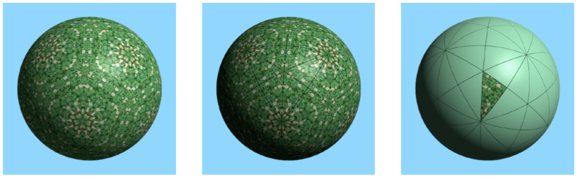
(a)

(b)

(c)

Figure 2: How to construct the *235 orbifold. (a) Begin with an icosahedrally symmetric pattern on the 2-sphere. (b) Locate all lines of mirror symmetry. Each is a great circle, and together they divide the sphere into 120 congruent triangles. (c) Fold the sphere along all mirror lines simultaneously, so that the whole sphere maps 120-to-1 onto a single triangle. The resulting quotient is the *235 orbifold. The Conway notation *235 may be understood as follows: the ‘*’ denotes the mirror-symmetric origin of the triangle’s sides, while the 2, the 3 and the 5 denote the fact that 2, 3 and 5 mirror lines met at each corner, respectively.

The quotient $S^{2}/I_{h}$ is an orbifold consisting of a spherical triangle with mirror boundaries and corner reflectors with angles $\pi/2$, $\pi/3$ and $\pi/5$ (see Figure 2). In Conway’s notation this orbifold is denoted *235.

• Each point in the interior of the triangle lifts to an invariant set of 120 points on $S^{2}$, which in turn defines an invariant set of 60 directions.

• However, each point on a mirror boundary lifts to only 60 points on $S^{2}$, defining only 30 directions. For this reason it’s convenient to think of a point on the mirror boundary as a “half-point”.

• A point at the corner reflector of angle $\pi/2$ lifts to 30 points on $S^{2}$ or 15 directions, so it’s convenient to think of it as a “quarter point”.

• Similarly, the points at the corner reflectors of angle $\pi/3$ and $\pi/5$ may be considered a $1/6$ point and a $1/10$ point, respectively.

In all cases, a $\frac{1}{F}$ fractional ($F=1,2,4,6$ or $10$) point of $S^{2}/I_{h}$ represents an invariant set of $\ell=\frac{60}{F}$ directions. Another way to think about it is that a half-point on the mirror boundary lifts to 120 half-points on $S^{2}$, and then each pair of identically positioned half-points combines to form a single full point, and similarly for the other fractional points.

Definition 6.1.1. Let

$C_{\frac{1}{10}}$ denote the number of $\frac{1}{10}$ points at the vertex of angle $\pi/5$,

$C_{\frac{1}{6}}$ denote the number of $\frac{1}{6}$ points at the vertex of angle $\pi/3$,

$C_{\frac{1}{4}}$ denote the number of $\frac{1}{4}$ points at the vertex of angle $\pi/2$,

$C_{\frac{1}{2}}$ denote the number of half points on the triangle’s perimeter, and

$C_{1}$ denote the number of whole points in the triangle’s interior.

The preceding discussion has shown that

Proposition 6.1.2. Each $I$-invariant equivalence class $[f]$ of modes of $S^{2}$ corresponds to a unique choice of $\ell$ $I$-invariant multipole vectors. The degree of a representative mode $f$ is

$$\ell\;=\;6C_{\frac{1}{10}}\;+\;10C_{\frac{1}{6}}\;+\;15C_{\frac{1}{4}}\;+\;30C_{\frac{1}{2}}\;+\;60C_{1}.$$ (24)

Some care is required here: knowing that an equivalence class $[f]$ of modes is $I$-invariant does not immediately imply that each representative $f$ of that class is $I$-invariant. It is a priori possible that some symmetry $\gamma\in I$ could send $f$ to $-f$. The next proposition shows that this does not happen.

Proposition 6.1.3. If an equivalence class $[f]$ of modes of $S^{2}$ is invariant under the icosahedral group $I$, then each representative $f$ is also invariant under $I$.

Proof. Let $\{d_{1},...,d_{\ell}\}$ be the set of $I$-invariant directions defining the class $[f]$ (Section 5.2), and let $\gamma\in I$ be a symmetry of the icosahedron. By the assumed $I$-invariance of $[f]$, we know that $\gamma$ sends each $d_{i}$ to $\pm d_{j}$ (for some $j$). To prove that $f$ itself is invariant, it suffices to prove that $\gamma$ sends $d_{i}$ to $-d_{j}$ (rather than to $+d_{j}$) for an even number of the $d_{i}$.

First consider the case that a given $d_{i}$ lies in the “interior” of the *235-orbifold (Figure 2c). This implies that 59 other $d_{i}$ (for different values of $i$) lie in the interiors of other copies of the fundamental triangle (Figure 2b), arranged symmetrically . Each right-handed copy of the fundamental triangle lies antipodally opposite a left-handed copy (Figure 2b). If we make the convention to orient each of the 60 $d_{i}$ in question so that it points toward a right-handed copy of the triangle and away from a left-handed copy, then every $\gamma\in I$ will preserve those $d_{i}$ exactly, always sending a $d_{i}$ to a $+d_{j}$, never to a $-d_{j}$.

Next consider the case that some $d_{i}$ lies on the perimeter (the mirror boundary) of the *235-orbifold’s fundamental triangle. In this case it has only 30 translates under the group (including itself). The icosahedral group $I$ consists entirely of rotations, each about some vertex of the tiling (Figure 2b). Let $\gamma$ be some such rotation. In the generic case that none of the 30 $d_{i}$ lies exactly $90^{\circ}$ from the rotation axis of $\gamma$, we may orient all 30 $d_{i}$ to point towards the “northern hemisphere” (relative to $\gamma$’s rotation axis) and away from the “southern hemisphere”. In this case $\gamma$ sends each $d_{i}$ to a $+d_{j}$, never to a $-d_{j}$. In the non-generic case that some of the $d_{i}$ lie exactly on the “equator” relative to $\gamma$’s rotation axis, consider the three sub-cases that the rotation $\gamma$ has order 2, 3 or 5. When $\gamma$ is a rotation of order 3 or 5, easy ad hoc conventions serve to orient the equatorial $d_{i}$ so that $\gamma$ respects their orientations. When $\gamma$ is a rotation of order 2, it perforce takes each $d_{i}$ to $-d_{i}$, but there are exactly two such $d_{i}$, so the net effect is still that $\gamma$ maps the mode $f$ to $+f$, not $-f$.

Finally, consider the case that some $d_{i}$ lies isolated at one of the fundamental triangle’s vertices. According to whether the vertex is a corner reflector of order 2, 3 or 5, $d_{i}$ will have 15, 10 or 6 translates (including itself), respectively. Imitating the method of the preceding paragraph, we consider a rotation $\gamma\in I$, and wherever possible orient the $d_{i}$ to point towards the northern hemisphere and away from the southern hemisphere, thus ensuring that $\gamma$ permutes such $d_{i}$ respecting orientation. It remains to consider only the $d_{i}$ that lie on the equator relative to $\gamma$’s rotation axis. When $\gamma$ has order 3 or 5, its equator contains corner reflectors of order 2 only, and an ad hoc convention serves to orient them consistently. When $\gamma$ has order 2, it maps each equatorial $d_{i}$ to $-d_{i}$, but the equator contains exactly four corner reflectors of order 2, four corner reflectors of order 3 and four corner reflectors of order 5, so in each sub-case the equator contains exactly two of the directions $d_{i}$ (from among the complete set of 15, 10 or 6 directions under consideration), and because exactly two directions get flipped, we conclude that $\gamma$ maps the mode $f$ to $+f$, not $-f$. $\blacksquare$

Corollary 6.1.4. Any value of $\ell$ not expressible in the form (24), for example $\ell=14$, cannot be the degree of an eigenmode of $S^{2}/I$.

Corollary 6.1.5. The nontrivial $I$-invariant mode of $S^{2}$ of least degree has degree $l=6$.

6.2 Dimension of the space of modes

Proposition 6.2.1. The $I$-invariant mode of degree $l=6$ is unique up to a constant multiple. Thus $dim(V^{6})=1$.

Proof. To construct this mode, take the *235 orbifold and place a single $1/10$ point at the corner reflector of angle $\pi/5$. This $1/10$ point lifts to 12 points of $S^{2}$ which in turn define 6 directions. According to Maxwell’s formula (23), those 6 directions define an $I$-invariant class of modes $[f]$ of degree 6. By Proposition 6.1.3, each representative $f$ of $[f]$ is $I$-invariant. Assuming a fixed realization of the icosahedral group $I$, the 6 directions are well defined — they align with the vertices of an icosahedron or the face centers of a dodecahedron. Therefore the class $[f]$ is also well defined, and the only degree of freedom for the mode $f$ is the scale factor inherent in the equivalence class $[f]$. Thus $V^{6}$ is of dimension 1. $\blacksquare$

The method of the preceding proposition lets us construct $I$-invariant modes of degree 10 (place a $1/6$ point at the corner reflector of angle $\pi/3$) and degree 15 (place a $1/4$ point at the corner reflector of angle $\pi/2$), while proving that $I$-invariant modes of most other low degrees cannot exist. $V^{10}$ and $V^{15}$ have dimension 1.

The case of degree 30, realized by placing a half-point on the *235 orbifold’s mirror boundary, is more interesting because we have an extra degree of freedom corresponding to where we choose to place the half-point. Allowing for the scale factor inherent in the equivalence class $[f]$ gives a total of two real degrees of freedom: $V^{30}$ has dimension 2.

The case of degree 60, corresponding to one full point in the *235 orbifold, is more interesting still, because now we have a choice as to how we realize that one full point:

• Case 1. We may place a single full point anywhere in the orbifold.

• Case 2. We may place two half-points on the orbifold’s mirror boundary. In the special case that the two half-points coincide, we get a single full point as in Case 1.

• Case 3. We may place any combination of fractional points at the orbifold’s corner reflectors, just so the fractions sum to one. However it turns out that the only ways to do this are to place a full point at a single corner (for example realized as ten 1/10 points at the corner of angle $\pi/5$) or to place a half-point at each of two corners (for example realized as five 1/10 points at the corner of angle $\pi/5$ plus three 1/6 points at the corner of angle $\pi/3$). The full point corresponds to Case 1 while the two half-points correspond to Case 2, so nothing new arises here and we will henceforth ignore this Case 3.

• Case 4. We may place a half-point on the mirror boundary and a half-point’s worth of fractional points at the corner reflectors, but as in Case 3 nothing new arises here so we may ignore this possibility.

Proposition 6.2.2. The $I$-invariant classes $[f]$ of modes of $S^{2}$ of degree $l=60$ are parameterized by a real projective plane.

Proof. Each class $[f]$ of degree 60 corresponds to 60 directions $\{d_{1},...,d_{60}\}$ that are invariant under the icosahedral group $I$, which in turn correspond either to a single point in the *235 orbifold (Case 1 above) or to a pair of half-points on the mirror boundary (Case 2 above).

The possible locations for a whole point are obviously parameterized by the points of the orbifold itself, which is topologically a disk.

The possible locations for a pair of points on the orbifold’s mirror boundary are parameterized by a Möbius strip. To see why, first note that the mirror boundary is topologically a circle $S^{1}$. Parameterize this circle in some arbitrary but fixed way, with the parameter angle defined modulo $2\pi$, and then for any pair of points define

$\theta$ = the position of the two points’ “center of mass” ($\theta\in S^{1}=\mathbb{R}/2\pi)$

$\phi$ = the separation between the two points ($\phi\in[0,\pi])$

At first glance this gives a cylinder parameterized by $(\theta,\phi)$. But $(\theta,\pi)$ and $(\theta+\pi,\pi)$ define the same pair of points, so we must identify opposite points on the cylinder’s upper boundary circle $(\theta,\pi)\sim(\theta+\pi,\pi)$, which transforms the cylinder into a Möbius strip. The cylinder’s lower boundary circle $(\theta,0)$ becomes the Möbius strip’s edge.

The Möbius strip’s edge, parameterized by $(\theta,0)$, corresponds to the case that the two half-points fuse together to form a single whole point on the triangle’s perimeter. This corresponds exactly to the boundary of the disk in the whole point parameter space. In other words, the total parameter space is the union of a disk and a Möbius strip glued together along their boundary circles, which yields a real projective plane. $\blacksquare$

It’s no surprise that the parameter space is a real projective plane. The space of $\Gamma$-invariant harmonic functions $f$ on $S^{2}$ of any fixed degree $\ell$ is a vector space of some finite dimension $n$. When we pass from functions $f$ to equivalence classes $[f]$ we identify each line through the origin to a single point, giving in all cases a real projective space $\mathbb{R}P^{n-1}$. In the case just considered, with degree $\ell=60$, we found the projective space to be $\mathbb{R}P^{2}$ meaning the total function space, including the scale factor, is $\mathbb{R}^{3}$.

To construct a generic $I$-invariant mode, we may place any combination of whole points (anywhere in the orbifold), half points (on the orbifold’s mirror boundary), and other fractional points (isolated at the orbifold’s corner reflectors). Each whole point contributes two degrees of freedom to the space of modes (corresponding to the point’s location in the 2-dimensional triangle), each half point contributes one degree of freedom (corresponding to its location along the triangle’s 1-dimensional perimeter), and each isolated fractional point contributes nothing. The overall scaling factor contributes one more degree of freedom for any nontrivial mode. In summary,

Proposition 6.2.3. The dimension of the space of $I$-invariant $\ell$-eigenmodes of $S^{2}$ is given by

$$dim(V^{\ell})=1+C_{\frac{1}{2}}+2C_{1}.$$ (25)

Note that no matter how many half points may or may not combine into whole points, the half and whole points together contribute $C_{\frac{1}{2}}+2C_{1}$ degrees of freedom.

6.3 Improved dimension formula

The dimension formula (25) is nice, but we would much rather have a formula in terms of $\ell$, to save us the trouble of manually decomposing $\ell$ into a linear combination of the $C_{i}$. Here is the improved formula,

Proposition 6.3.1. The dimension of the space of $I$-invariant $\ell$-eigenmodes of $S^{2}$ is given by

$$dim(V^{\ell})=1+\lfloor\frac{\ell}{2}\rfloor+\lfloor\frac{\ell}{3}\rfloor+\lfloor\frac{\ell}{5}\rfloor-\ell.$$ (26)

Proof. Recall that

$$\ell\;=\;6C_{\frac{1}{10}}\;+\;10C_{\frac{1}{6}}\;+\;15C_{\frac{1}{4}}\;+\;30C_{\frac{1}{2}}\;+\;60C_{1}.$$ (27)

and consider how the $C_{i}$ depend on $\ell$.

First consider $C_{\frac{1}{10}}$, the number of $\frac{1}{10}$ points. Taking Equation (27) modulo 5 we get

$$\ell\equiv C_{\frac{1}{10}}\;\rm{(mod\,5)}.$$

But the number of isolated $\frac{1}{10}$ points may only be 0, 1, 2, 3 or 4, because if we had 5 or more $\frac{1}{10}$ points they would combine to form half points and acquire an additional degree of freedom. So the number of isolated $\frac{1}{10}$ points must be $C_{\frac{1}{10}}=\ell-5\lfloor\frac{\ell}{5}\rfloor$. The same argument, repeated mod 3 and mod 2, gives $C_{\frac{1}{6}}=\ell-3\lfloor\frac{\ell}{3}\rfloor$ and $C_{\frac{1}{4}}=\ell-2\lfloor\frac{\ell}{2}\rfloor$, respectively.

Rearranging Equation (27) now gives

$$C_{\frac{1}{2}}+2C_{1} = \frac{1}{30}\left[\ell-6C_{\frac{1}{10}}-10C_{\frac{1}{6}}-15C_{\frac{1}{4}}\right]$$ (28)

$$= \frac{1}{30}\left[\ell-6\left(\ell-5\lfloor\frac{\ell}{5}\rfloor\right)-10\left(\ell-3\lfloor\frac{\ell}{3}\rfloor\right)-15\left(\ell-2\lfloor\frac{\ell}{2}\rfloor\right)\right]$$

$$= \lfloor\frac{\ell}{5}\rfloor+\lfloor\frac{\ell}{3}\rfloor+\lfloor\frac{\ell}{2}\rfloor-\ell$$

Substituting Equation (28) into Equation (25) gives the final result (26) as stated above. $\blacksquare$

This agrees with Ikeda’s formula [2], while at the same time providing a concrete construction of the modes and shedding additional light on the formula’s geometrical origins, as degrees of freedom in an orbifold.

7 Conclusion

Returning to the 3-dimensional Poincaré dodecahedral space $S^{3}/I^{*}$, the results of the preceding sections may be summarized as follows. Keep in mind that $S^{3}/I^{*}$ admits $k$-modes for even $k$ only; odd $k$-modes cannot exist because $I^{*}$ contains the antipodal map.

Theorem 7.1 To construct the modes of the Poincaré dodecahedral space $S^{3}/I^{*}$,

• Each mode of $S^{3}/I^{*}$ corresponds to an $I^{*}$-invariant mode of $S^{3}$ (elementary).

• Each $I^{*}$-invariant mode of $S^{3}$ is a sum of twists of $I^{*}$-invariant vertical modes of $S^{3}$ (Proposition 4.1.1).

• Each $I^{*}$-invariant vertical $k$-mode of $S^{3}$ is the pull-back, under the Hopf map, of an $I$-invariant $\ell$-mode of $S^{2}$, with $k=2\ell$ (Proposition 3.2.1).

• The $I$-invariant $\ell$-modes of $S^{2}$ are parameterized by $\ell/60$ points on the *235-orbifold, possibly including fractional points (Section 6.1).

Theorem 7.2 The space of $k$-modes of the Poincaré dodecahedral space $S^{3}/I^{*}$ has dimension

$$(k+1)(1+\lfloor\frac{k/2}{2}\rfloor+\lfloor\frac{k/2}{3}\rfloor+\lfloor\frac{k/2}{5}\rfloor-\frac{k}{2}).$$ (29)

Proof. The space of $I$-invariant $k/2$-modes of the 2-sphere has dimension $1+\lfloor\frac{k/2}{2}\rfloor+\lfloor\frac{k/2}{3}\rfloor+\lfloor\frac{k/2}{5}\rfloor-\frac{k}{2}$ (Proposition 6.3.1) and thus the space of vertical $I^{*}$-invariant $k$-modes of the 3-sphere has this same dimension (Theorem 7.1). The twist operators then take each vertical mode to a $(k+1)$-dimensional space of generic $I$-invariant modes (Table 1 and Proposition 4.1.1,), completing the proof. $\blacksquare$

References

- [1] Cosmic Topology, Lachièze-Rey M. & Luminet J.P. 1994, Physics Reports 1994, 254,3 (http://arxiv.org/abs/gr-qc/9605010v2)
- [2] A. Ikeda, On the spectrum of homogeneous spherical space forms, Kodai Math. J. 18 (1995), 57-67
- [3] Laplacan eigenmodes for spherical spaces, M. Lachièze-Rey and S. Caillerie 2005, Class. Quantum Grav. 22 (2005) 695-708. (http://arxiv.org/abs/astro-ph/0501419)
- [4] Predicting the CMB power spectrum for binary polyhedral spaces, Gundermann J. (http://arxiv.org/abs/astro-ph/0503014)
- [5] Eigenmodes of Dodecahedral space, Lachièze-Rey M. 2004, CQG, vol.21, 9, p 2455-2464 (http://arxiv.org/abs/gr-qc/0402035)
- [6] Weeks J., Exact polynomial eigenmodes for homogeneous spherical 3- manifolds, Classical and Quantum Gravity 23 (2006) 6971–6988 (http://arxiv.org/abs/math/0502566v3)
- [7] James Clerk Maxwell, A Treatise on Electricity and Magnetism, ed. 1873, ed. 1891, reprinted by Dover Publications, 1954.
-
[8]
Dennis, M. R. 2004, J. Phys. A, 37, 9487 (math-ph/0408046)
2005, J. Phys. A, 38, 1653 (http://arxiv.org/abs/math-ph/0410004) - [9] Copi, C. J., Huterer, D., & Starkman, G. D. 2004, Phys. Rev. D, 70, 043515 (http://arxiv.org/abs/astro-ph/0310511)
- [10] Katz, G., & Weeks, J. 2004, Phys. Rev. D, 70, 063527 (http://arxiv.org/abs/astro-ph/0405631)
- [11] Land, K., & Magueijo, J. 2005a, Phys. Rev. Lett., 95, 071301 (http://arxiv.org/abs/astro-ph/0502237)
- [12] Lachièze-Rey M. 2004 (http://arxiv.org/abs/astro-ph/0409081
- [13] Weeks, J. R. 2004, (http://arxiv.org/abs/astro-ph/0412231