Polarization analysis of gravitational-wave backgrounds from the correlation signals of ground-based interferometers: measuring a circular-polarization mode

Abstract

The Stokes $V$ parameter characterizes asymmetry of amplitudes between right- and left-handed waves, and non-vanishing value of the $V$ parameter yields a circularly polarized signal. Cosmologically, $V$ parameter may be a direct probe for parity violation in the universe. In this paper, we theoretically investigate a measurement of this parameter, particularly focusing on the gravitational-wave backgrounds observed via ground-based interferometers. In contrast to the traditional analysis that only considers the total amplitude (or equivalently $\Omega_{\rm GW}$), the signal analysis including a circular-polarized mode has a rich structure due to the multi-dimensionality of target parameters. We show that, by using the network of next-generation detectors, separation between polarized and unpolarized modes can be performed with small statistical loss induced by their correlation.

I Introduction

Because of the extremely weak signal, a direct detection of gravitational waves is a technically challenging issue, and we have not yet succeeded the direct detection despite extensive efforts. Nevertheless, the weakness of the gravitational interaction may be a great advantage for astronomy and cosmology, because gravitational waves can propagate to us from very early universe almost without scattering and absorption Thorne_K:1987 ; Cutler:2002me . In this respect, stochastic background of gravitational waves is one of the most important targets for gravitational wave astronomy Allen:1996vm . If detected, the stochastic background will serve as an invaluable fossil to study the physics at extremely high-energy scale for which other methods cannot be attainable.

Over the last decade, sensitivity of gravitational wave detectors to the stochastic background has drastically improved. We will soon reach at the sensitivity level $\Omega_{\rm GW}\lesssim 10^{-5}$ around 100Hz Abbott:2006zx , where $\Omega_{\rm GW}$ is the energy density of the gravitational waves normalized by critical density of the universe. This level is below the indirect cosmological constraints, such as derived from the observed abundance of light elements Allen:1996vm (see Smith:2006nka for the constraints from cosmic microwave background), and in this sense, gravitational wave detectors will provide a unique opportunity to directly constrain the early universe. In order to further get a stringent constraint and/or valuable information from the next-generation detectors, one important approach is to improve the statistical analysis of gravitational wave backgrounds. So far, most of theoretical studies on the gravitational-wave backgrounds have been directed to its energy spectrum (for its anisotropies, see, e.g., Giampieri:1997ie ). The authors recently provided a brief sketch for measurement of the Stokes $V$ parameter of the gravitational-wave background via correlation analysis of ground-based detectors Seto:2007tn (see Lue:1998mq for cosmic microwave background and Seto:2006hf for space gravitational wave detectors such as LISA lisa or BBO/DECIGO bbo ; Seto:2001qf ). The Stokes $V$ parameter may be basic observable to quantify the parity violation process. One of such parity violation process is through the Chern-Simons term that might be originated from string theory Alexander:2004us . This paper is a follow-up study to the preceding short report. In addition to detailed explanations and supplementary materials to the previous paper, we developed a new statistical framework to deal with multiple parameters of gravitational wave backgrounds, and we specifically applied it to simultaneous estimation of amplitudes of both the unpolarized and polarized modes of the gravitational-wave background.

This paper is organized as follows. In section II, we describe polarization decomposition of a gravitational-wave background, and define its Stokes $V$ parameter. The basic framework to treat polarized gravitational waves is essentially the same one as in the case of electromagnetic waves radipro . In section III, we explain the correlation analysis for the gravitational-wave background and introduce the overlap functions that characterize sensitivities to the polarized and unpolarized modes. Then, we discuss basic properties of the overlap functions, and calculate them for the planed next-generation detectors, such as advanced LIGO. In section IV, broadband analysis of the gravitational-wave background is studied, taking into account the measurement noises for each detector. In section V, we discuss how well we can separately measure the polarized and unpolarized modes. In contrast to the traditional arguments only for the unpolarized mode, the situation considered here is more complicated. We provide a statistical framework to analyze multiple parameters of the stochastic background with correlation analysis. Finally, section VI is a brief summary of this paper. Appendix A presents the derivation for the expressions of the overlap functions. This geometrical derivation is similar to that given in Ref.Flanagan:1993ix . In appendix B, we discuss the probability distribution functions (PDFs) of basic observational quantities with correlation analysis. In appendix C, we derive the formal expressions for optimal signal-to-noise ratios for detectors more than four. In appendix D, we comment on the surface of the Moon as potential sites for laser interferometers.

II Circular polarization

Let us first describe the polarization states of stochastic gravitational waves. We consider a plane wave expansion of gravitational-wave backgrounds as

$$h_{ij}(t,{\mbox{\boldmath${x}$}})=\sum_{P=+,\times}\int^{\infty}_{-\infty}df\int_{S^{2}}d\mbox{\boldmath${n}$}~{}h_{P}(f,\mbox{\boldmath${n}$})e^{2\pi if(-t+\mbox{\boldmath${n}$}\cdot{\mbox{\boldmath${x}$}})}{\mbox{\boldmath${e}$}}^{P}_{ij}(\mbox{\boldmath${n}$}).$$ (1)

Here, the bases for transverse-traceless tensor ${\mbox{\boldmath${e}$}}^{P}$ $(P=+,\times)$ are given as

$${\mbox{\boldmath${e}$}}^{+}={\hat{\mbox{\boldmath${e}$}}}_{\theta}\otimes{\hat{\mbox{\boldmath${e}$}}}_{\theta}-{\hat{\mbox{\boldmath${e}$}}}_{\phi}\otimes{\hat{\mbox{\boldmath${e}$}}}_{\phi},\quad{\mbox{\boldmath${e}$}}^{\times}={\hat{\mbox{\boldmath${e}$}}}_{\theta}\otimes{\hat{\mbox{\boldmath${e}$}}}_{\phi}+{\hat{\mbox{\boldmath${e}$}}}_{\phi}\otimes{\hat{\mbox{\boldmath${e}$}}}_{\theta}$$ (2)

with the unit vectors ${\hat{\mbox{\boldmath${e}$}}}_{\theta}$ and ${\hat{\mbox{\boldmath${e}$}}}_{\phi}$ being normal to the propagation direction ${n}$ that are associated with a right-handed Cartesian coordinate:

$${\hat{\mbox{\boldmath${e}$}}}_{\theta}=(\cos\theta\cos\phi,\cos\theta\sin\phi,-\sin\theta),~{}~{}{\hat{\mbox{\boldmath${e}$}}}_{\phi}=(-\sin\phi,\cos\phi,0).$$ (3)

On the other hand, the random amplitude $h_{P}$ represents the mode coefficients and the statistical properties of it are characterized by the power spectral density given by $\left\langle h_{P1}(\mbox{\boldmath${n}$})h_{P2}^{*}(\mbox{\boldmath${n}$}^{\prime})\right\rangle$ $(P1,P2=+,\times)$ for two polarization modes as

$$\left(\begin{array}[]{@{\,}cc@{\,}}\left\langle h_{+}(f,\mbox{\boldmath${n}$})h_{+}^{*}(f^{\prime},\mbox{\boldmath${n}$}^{\prime})\right\rangle&\left\langle h_{+}(f,\mbox{\boldmath${n}$})h_{\times}^{*}(f^{\prime},\mbox{\boldmath${n}$}^{\prime})\right\rangle\\ \left\langle h_{\times}(f,\mbox{\boldmath${n}$})h_{+}^{*}(f^{\prime},\mbox{\boldmath${n}$}^{\prime})\right\rangle&\left\langle h_{\times}(f,\mbox{\boldmath${n}$})h_{\times}^{*}(f^{\prime},\mbox{\boldmath${n}$}^{\prime})\right\rangle\\ \end{array}\right)=\frac{1}{2}{\delta_{\rm D}^{2}(\mbox{\boldmath${n}$}-\mbox{\boldmath${n}$}^{\prime})\delta_{\rm D}(f-f^{\prime})}\left(\begin{array}[]{@{\,}cc@{\,}}I(f,\mbox{\boldmath${n}$})+Q(f,\mbox{\boldmath${n}$})&U(f,\mbox{\boldmath${n}$})-iV(f,\mbox{\boldmath${n}$})\\ U(f,\mbox{\boldmath${n}$})+iV(f,\mbox{\boldmath${n}$})&I(f,\mbox{\boldmath${n}$})-Q(f,\mbox{\boldmath${n}$})\\ \end{array}\right),$$ (4)

with delta functions $\delta_{\rm D}(\cdot)$ and the notation $\left\langle\cdots\right\rangle$ for an ensemble average. Here, the quantities $I,Q,U$ and $V$ are the Stokes parameters and are real functions of direction ${n}$. Alternative to the linear polarization bases $({\mbox{\boldmath${e}$}}^{+},{\mbox{\boldmath${e}$}}^{\times})$, we may use the circular polarization bases $({\mbox{\boldmath${e}$}}^{R},{\mbox{\boldmath${e}$}}^{L})$ (right- and left-handed modes)

$${\mbox{\boldmath${e}$}}^{R}=\frac{({\mbox{\boldmath${e}$}}^{+}+i{\mbox{\boldmath${e}$}}^{\times})}{\sqrt{2}},\quad{\mbox{\boldmath${e}$}}^{L}=\frac{({\mbox{\boldmath${e}$}}^{+}-i{\mbox{\boldmath${e}$}}^{\times})}{\sqrt{2}}$$ (5)

for the plane wave expansion (1). Two coefficients $h_{R,L}$ for the corresponding modes are given as

$$h_{R}=\frac{(h_{+}-ih_{\times})}{\sqrt{2}},~{}~{}~{}h_{L}=\frac{(h_{+}+ih_{\times})}{\sqrt{2}}.$$ (6)

Then the covariance matrix is recast as

$$\left(\begin{array}[]{@{\,}cc@{\,}}\left\langle h_{R}(f,\mbox{\boldmath${n}$})h_{R}(f^{\prime},\mbox{\boldmath${n}$}^{\prime})^{*}\right\rangle&\left\langle h_{L}(f,\mbox{\boldmath${n}$})h_{R}(f^{\prime},\mbox{\boldmath${n}$}^{\prime})^{*}\right\rangle\\ \left\langle h_{R}(f,\mbox{\boldmath${n}$})h_{L}(f^{\prime},\mbox{\boldmath${n}$}^{\prime})^{*}\right\rangle&\left\langle h_{L}(f,\mbox{\boldmath${n}$})h_{L}(f^{\prime},\mbox{\boldmath${n}$}^{\prime})^{*}\right\rangle\\ \end{array}\right)=\frac{1}{2}{\delta_{\rm D}({\mbox{\boldmath${n}$}-\mbox{\boldmath${n}$}^{\prime}})^{2}\delta_{\rm D}({f-f^{\prime}})}\left(\begin{array}[]{@{\,}cc@{\,}}I(f,\mbox{\boldmath${n}$})+V(f,\mbox{\boldmath${n}$})&Q(f,\mbox{\boldmath${n}$})-iU(f,\mbox{\boldmath${n}$})\\ Q(f,\mbox{\boldmath${n}$})+iU(f,\mbox{\boldmath${n}$})&I(f,\mbox{\boldmath${n}$})-V(f,\mbox{\boldmath${n}$})\\ \end{array}\right).$$ (7)

With this expression, it is apparent that the real parameter $V$ characterizes the asymmetry of amplitudes between right- and left-handed waves, while the parameter $I(\geq|V|)$ represents their total amplitude. For example, if we can observationally establish $V>0$, the background is dominated by right-handed waves. Since the parity transformation interchanges the two polarization modes, the asymmetry is closely related to parity violation process (see e.g. Alexander:2004us ; Kahniashvili:2005qi for recent theoretical studies). Therefore, we may detect signature of parity violation in the early universe by analyzing the $V$ parameter of gravitational-wave backgrounds. This is the basic motivation of this paper.

Since the two parameters $I$ and $V$ have spin 0, their angular dependence can be expanded by the standard (scalar) spherical harmonics $Y_{\ell m}$:

$$I(f,\mbox{\boldmath${n}$})=\sum_{\ell=0}^{\infty}\sum_{m=-\ell}^{\ell}I_{\ell m}(f)Y_{\ell m}(\mbox{\boldmath${n}$}),\quad V(f,\mbox{\boldmath${n}$})=\sum_{\ell=0}^{\infty}\sum_{m=-\ell}^{\ell}V_{\ell m}(f)Y_{\ell m}(\mbox{\boldmath${n}$}).$$ (8)

On the other hand, the combinations $Q\pm iU$ describe the linear polarization and have spin $\pm 4$ reflecting spin-2 nature of gravitational waves. They are expanded with the spin-weighted spherical harmonics as

$$(Q+i\,U)(f,\mbox{\boldmath${n}$})=\sum_{\ell=4}^{\infty}\sum_{m=-\ell}^{\ell}P^{+}_{\ell m}(f){}_{4}Y_{\ell m}(\mbox{\boldmath${n}$}),\quad(Q-i\,U)(f,\mbox{\boldmath${n}$})=\sum_{\ell=4}^{\infty}\sum_{m=-\ell}^{\ell}P^{-}_{\ell m}(f){}_{-4}Y_{\ell m}(\mbox{\boldmath${n}$}).$$ (9)

Note that $Q\pm i\,U$ do not have monopole components ($\ell=0$), because the linear modes introduce specific spatial directions. Since the observed universe is highly homogeneous and isotropic on large spatial scales, it is reasonable to set the monopole modes of a cosmological stochastic background as our primary targets. Therefore, in this paper, we do not study the linear polarization $Q\pm i\,U$. From the same reason, we also neglect the directional dependence of the $I$ and $V$ modes.

Next, we describe the frequency dependence of the gravitational-wave background. To characterize the gravitational waves in the cosmological context, rather than the spectral density, the normalized logarithmic energy density of the stochastic background, $\Omega_{\rm GW}(f)$, is frequently used in the literature Flanagan:1993ix ; Allen:1997ad . The density $\Omega_{\rm GW}(f)$ is defined by the spectral density $I$ as

$$\Omega_{\rm GW}(f)=\frac{4\pi^{2}f^{3}}{\rho_{c}}I(f),$$ (10)

where $\rho_{\rm c}(=3H_{0}^{2}/8\pi$, $H_{0}=70h_{70}$km/sec/Mpc: the Hubble parameter) is the critical density of the universe. We also define the polarization degree by $\Pi(f)=V(f)/I(f)$. In terms of the quantities $\Omega_{\rm GW}(f)$ and $\Pi(f)$, the asymmetry parameter $V$ is expressed as

$$V(f)=\frac{\rho_{\rm c}}{4\pi^{2}f^{3}}\Omega_{\rm GW}(f)\Pi(f).$$ (11)

III Overlap functions for ground-based detectors

This section discusses the overlap functions for correlation signals as the basic ingredient for correlation analysis of gravitational-wave background. In Sec.III.1, the definition and the analytic formula for overlap functions are given. Subsequently, Sec.III.2, III.3 and III.4 discuss special or limiting cases for overlap functions in order to understand their geometrical properties. After describing some mathematical properties in Sec.III.5, we evaluate the overlaps functions for specific pairs of five detectors in Sec.III.6.

III.1 Formulation

Let us begin by considering how we can detect the monopole components of the $I$ and $V$ modes with laser interferometers. Response $H_{a}$ of a detector $a$ at ${\mbox{\boldmath${x}$}}_{a}$ is written as

$$H_{a}(f)=\int_{S^{2}}d\mbox{\boldmath${n}$}\sum_{P=+,\times}h_{P}(f,\mbox{\boldmath${n}$})F^{P}_{a}(\mbox{\boldmath${n}$},f)e^{2\pi if\mbox{\boldmath${n}$}\cdot{\mbox{\boldmath${x}$}}_{a}}.$$ (12)

The function $F_{a}^{P}$ is the beam pattern function and it represents the response of the detector to each linear polarization mode. Here we used the conventional linear polarization bases.

To distinguish the background signals from detector noises and to obtain a large signal-to-noise ratio, the correlation analysis with multiple detectors is essential m87 ; Christensen:1992wi ; Flanagan:1993ix ; Allen:1997ad . We define the correlation $C_{ab}(f)$ of data streams obtained from two detectors $a$ and $b$ as

$$\left\langle H_{a}(f)H_{b}(f^{\prime})^{*}\right\rangle\equiv C_{ab}(f)\delta_{\rm D}(f-f^{\prime}).$$ (13)

Keeping the monopole contribution only, its expectation value is written as

$$C_{ab}(f)=\frac{8\pi}{5}\left[\gamma_{I,ab}(f)I(f)+\gamma_{V,ab}(f)V(f)\right],$$ (14)

where $\gamma_{I}$ is the overlap function and given by Flanagan:1993ix ; Allen:1997ad

$$\gamma_{I,ab}(f)=\frac{5}{8\pi}\int_{S^{2}}d\mbox{\boldmath${n}$}\left[\left\{F_{a}^{+}F_{b}^{+*}+F_{a}^{\times}F_{b}^{\times*}\right\}e^{iy\mbox{\boldmath${n}$}\mbox{\boldmath${m}$}}\right],$$ (15)

with rewriting ${\mbox{\boldmath${x}$}}_{a}-{\mbox{\boldmath${x}$}}_{b}=D\mbox{\boldmath${m}$}$ ($D$: distance, ${m}$: unit vector) and $y\equiv 2\pi fD/c$. The variable $y$ represents the phase difference at two cites $a$ and $b$ for waves with a propagation direction ${m}$. Similarly, the function $\gamma_{V,ab}(f)$ is given by

$$\gamma_{V,ab}(f)=\frac{5}{8\pi}\int_{S^{2}}d\mbox{\boldmath${n}$}\left[i\left\{F_{a}^{+}F_{b}^{\times*}-F_{a}^{\times}F_{b}^{+*}\right\}e^{iy\mbox{\boldmath${n}$}\mbox{\boldmath${m}$}}\right].$$ (16)

Two functions $\gamma_{I}$ and $\gamma_{V}$ are purely determined by relative configuration of two detectors.

Here, we summarize the response of ground-based L-shaped interferometer $a$. We assume that two arms of the next-generation interferometer have equal length with opening angle of $90^{\circ}$. We denote the unit vectors for the directions of its two arms as ${u}$ and ${v}$. At the frequency regime where the wavelength of the incident gravitational wave is much longer than the armlength, the beam pattern function takes a simple form as

$$F_{a}^{P}={\mbox{\boldmath${d}$}}_{a}:{\mbox{\boldmath${e}$}}^{P}(\mbox{\boldmath${n}$}),$$ (17)

where the colon represents a double contraction and the detector tensor ${\mbox{\boldmath${d}$}}_{a}$ is given by

$${\mbox{\boldmath${d}$}}_{a}=\frac{({{\mbox{\boldmath${u}$}}}_{a}\otimes{{\mbox{\boldmath${u}$}}}_{a}-{{\mbox{\boldmath${v}$}}}_{b}\otimes{{\mbox{\boldmath${v}$}}}_{b})}{2}.$$ (18)

In reality, there might be some exceptional cases that the opening angle of two arms is slightly different from $90^{\circ}$ such as GEO600, whose opening angle is $94.3^{\circ}$ Willke:2002bs . However, the response of such a detector can be treated as the one of the right-angled interferometer (see eg. lisa for the case with LISA).

Note that from equations (17) and (18), we have

$$\frac{5}{8\pi}\int_{S^{2}}d\mbox{\boldmath${n}$}\left[F_{i}^{+}F_{i}^{+*}\right]=\frac{5}{8\pi}\int_{S^{2}}d\mbox{\boldmath${n}$}\left[F_{i}^{\times}F_{i}^{\times*}\right]=\frac{1}{2},$$ (19)

and Schwartz inequality implies

$$-1\leq\gamma_{I,ab}\leq 1,~{}~{}~{}-1\leq\gamma_{V,ab}\leq 1.$$ (20)

In Table 1, we list positions and orientations of the ongoing (and planned) kilometer-size interferometers, AIGO aigo , LCGT Kuroda:1999vi , LIGO-Hanford, LIGO-Livingston Abramovici:1992ah , and Virgo Acernese:2002bw . As a reference, we also list two sub-kilometer-size interferometers, TAMA300 Ando:2001ej and GEO600 Willke:2002bs . We use a spherical coordinate system $(\theta,\phi)$ with which the north pole is at $\theta=0^{\circ}$, and $\phi$ represents longitude. The orientation $\alpha$ is the angle between the local east direction and the bisecting line of two arms of each detector measured counterclockwise. Since the beam pattern functions have spin-2 character with respect to the rotation of detector, meaningful information here is the angle $\alpha$ module $90^{\circ}$. In what follows, we mainly focus on the first five detectors in Table 1 with their abbreviations (A,C,H,L,V) and with $R=R_{\rm E}=6400$km for the radius of the Earth , but in section IV.3, we also discuss the detectors placed on the Moon as an exceptional but interesting case (see also appendix D).

	$\theta$	$\phi$	$\alpha$
AIGO (A)	$121.4$	$115.7$	$-45.0$
LCGT (C)	$53.6$	$137.3$	$70.0$
LIGO Hanford (H)	$43.5$	$-119.4$	$171.8$
LIGO Livingston (L)	$59.4$	$-90.8$	$243.0$
Virgo (V)	$46.4$	$10.5$	$116.5$
TAMA300	$54.3$	$139.5$	$225.0$
GEO600	$47.7$	$9.8$	$68.8$

Table 1: Positions $(\theta,\phi)$ and orientation angles $\alpha$ of detectors (in units of degree) on the Earth.

For the monopole modes of the stochastic background, only the relative configuration of two detectors is relevant with the correlation $C_{ab}$ and we do not need to deal with their overall rotation. Therefore, without loss of generality, their configuration is characterized by the three angular parameters $(\beta,\sigma_{1},\sigma_{2})$, shown in Figure 1 Flanagan:1993ix . Here, $\beta$ is the separation angle between two detectors measured from the center of the Earth. The angle $\sigma_{1}$ ($\sigma_{2}$) is the orientation of the bisector of two arms of the detector $a$ ($b$ respectively) measured in counter-clockwise manner relative to the great circle connecting $a$ and $b$. Their distance is given by $D=2R_{\rm E}\sin(\beta/2)$ that determines a characteristic frequency $f_{\rm D}\equiv c/D$ for the overlap functions. Following Flanagan:1993ix , we define the angles

$$\Delta\equiv\frac{({\sigma_{1}+\sigma_{2}})}{2},\quad\delta\equiv\frac{({\sigma_{1}-\sigma_{2}})}{2},$$ (21)

and the geometrical information for possible pairs made from the five detectors are summarized in Table 2.

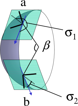
Figure 1: Detector planes are tangential to a sphere. Two detectors $a$ and $b$ are separated by the angle $\beta$ measured from the center of the sphere. The angles $\sigma_{1}$ and $\sigma_{2}$ describe the orientation of bisectors of interferometers in a counter-clockwise manner relative to the great circle joining two sites.

	A	C	H	L	V
AIGO (A)	$*$	$70.8,\,58.1,\,31.4$	$135.6,\,53.7,\,45.1$	$157.3,\,38.0,\,2.08$	$121.4,\,19.2,\,60.8$
LCGT (C)	$-0.61,\,-0.58,\,0.81$	$*$	$72.4,\,89.1,\,25.6$	$99.2,\,42.4,\,68.1$	$86.6,\,28.9,\,5.6$
LIGO Hanford (H)	$-0.82,\,-1.00,\,-0.007$	$1.0,\,-0.21,\,0.98$	$*$	$27.2,\,45.3,\,62.2$	$79.6,\,61.8,\,55.1$
LIGO Livingston (L)	$-0.88,\,0.99,\,0.15$	$-0.98,\,0.04,\,-1.0$	$-1.00,\,-0.36,\,-0.93$	$*$	$76.8,\,26.7,\,83.1$
Virgo (V)	$0.23,\,-0.45,\,-0.89$	$-0.43,\,0.92,\,0.38$	$-0.43,\,-0.76,\,-0.65$	$-0.29,\,0.89,\,-0.46$	$*$

Table 2: Upper right: angle parameters $(\beta,\delta,\Delta)$ for each pair of detectors in units of degree. Lower left: numerical values $(\cos(4\delta),\cos(4\Delta),\sin(4\Delta))$ for each pair of detectors.

The angular integral (15) can be performed analytically with explicit forms of the pattern functions, and we get

$$\gamma_{I,ab}=\Theta_{1}(y,\beta)\cos(4\delta)+\Theta_{2}(y,\beta)\cos(4\Delta),$$ (22)

with

$$\Theta_{1}(y,\beta)=\cos^{4}\left(\frac{\beta}{2}\right)\left(j_{0}+\frac{5}{7}j_{2}+\frac{3}{112}j_{4}\right),$$ (23)

and

$$\Theta_{2}(y,\beta)=\left(-\frac{3}{8}j_{0}+\frac{45}{56}j_{2}-\frac{169}{896}j_{4}\right)+\left(\frac{1}{2}j_{0}-\frac{5}{7}j_{2}-\frac{27}{224}j_{4}\right)\cos\beta+\left(-\frac{1}{8}j_{0}-\frac{5}{56}j_{2}-\frac{3}{896}j_{4}\right)\cos(2\beta).$$ (24)

The function $j_{n}$ is the $n$-th spherical Bessel function with its argument

$$y\equiv\frac{2\pi fD}{c}=\frac{4\pi fR_{\rm E}}{c}\,\sin\left(\frac{\beta}{2}\right).$$ (25)

The expression (22) coincides with the formula (4.1) in Ref. Flanagan:1993ix .

In a similar manner, the overlap function for the $V$ mode is given by

$$\gamma_{V,ab}=\Theta_{3}(y,\beta)\sin(4\Delta)$$ (26)

with

$$\Theta_{3}(y,\beta)=-\sin\left(\frac{\beta}{2}\right)\left[\left(-j_{1}+\frac{7}{8}j_{3}\right)+\left(j_{1}+\frac{3}{8}j_{3}\right)\cos\beta\right].$$ (27)

Note that the dependence of the angles $\delta$ and $\Delta$ on the overlap functions (22) and (26) can be deduced from the symmetric reasons Seto:2007tn .

In appendix A, we present a brief sketch to derive the expressions $\gamma_{I}$ and $\gamma_{V}$, using the symmetries of tensorial structure. Since our primary interest here is the dependence on the frequency $f$ and the angle $\beta$, we mainly use the set of the variables $(f,\beta)$, instead of $(y,\beta)$.

III.2 Special cases and asymptotic profiles

In order to get a physical insight into the overlap functions, it is instructive to consider geometrically simple configurations for two detectors. When a pair of detectors are placed on the same plane ($\beta=0^{\circ}$) and at the same position ($D=0$), we have the identity $(\Theta_{1},\Theta_{2})=(1,0)$ and thus $\gamma_{I,ab}=\cos(4\delta)$. In contrast, for $V$ mode, we obtain $\gamma_{V,ab}=0$ for the coplanar configuration $(\beta=0^{\circ})$ and this is even true with finite separation $D\neq 0$. The reason for this is explained in next subsection. Equation (22) and the identity $\Theta_{2}(y,0^{\circ})=0$ indicates that the function $\gamma_{I}$ depends very weakly on the parameter $\Delta$ at small angle $\beta\ll 180^{\circ}$. For ground-based detectors, the functions $\Theta_{i}(y,\beta)$ depend on the angle $\beta$ also through the variable $y=4\pi R_{\rm E}f\sin(\beta/2)/c$. Taking into account this fact, we obtain the following asymptotic profiles at small $\beta$ (in unit of radian):

$$\Theta_{1}=O(\beta^{0}),\quad\Theta_{2}=O(\beta^{4}),\quad\Theta_{3}=O(\beta^{3}).$$ (28)

On the other hand, for pair of detectors located at antipodal positions ($\beta=\pi$), the overlap function $\gamma_{I,ab}$ does not depend on the parameter $\delta$ because of $\Theta_{1}(y,180^{\circ})=0$. In this case, the asymptotic profiles become

$$\Theta_{1}=O((\pi-\beta)^{4}),\quad\Theta_{2}=O((\pi-\beta)^{0}),\quad\Theta_{3}=O((\pi-\beta)^{0}).$$ (29)

Note that at $\beta=0$ and $\pi$, we have

$$\partial_{\beta}\Theta_{1}=\partial_{\beta}\Theta_{2}=\partial_{\beta}\Theta_{3}=0.$$ (30)

III.3 Coplanar configuration

An L-shaped detector measures difference of spatial deformation towards its orthogonal two arms. This is purely geometrical measurement. If two detectors are placed on the same plane $z=0$, there is an apparent geometrical symmetry for the system with respect to the plane. Due to the mirror symmetry to the plane, a right-handed wave coming from the direction $(n_{x},n_{y},n_{z})$ and a left-handed wave from the direction $(n_{x},n_{y},-n_{z})$, provide an identical correlation signal, if they have the same frequency and amplitude. Therefore, for an isotropic background, right-handed waves coming from two directions $(n_{x},n_{y},\pm n_{z})$ exactly cancel out in the correlation signal. The same is true for left-handed waves. As a result, the symmetric system has no sensitivity to the isotropic component of the $V$-mode Seto:2007tn ; Seto:2006hf . We can directly confirm this cancellation from the definition (16) and the following relations

$$F^{+}_{i}(n_{x},n_{y},n_{z})=F^{+}_{i}(n_{x},n_{y},-n_{z}),\quad F^{\times}_{i}(n_{x},n_{y},n_{z})=-F^{\times}_{i}(n_{x},n_{y},-n_{z}),$$ (31)

which are easily derived from the symmetries of the polarization bases $e^{+,\times}(\mbox{\boldmath${n}$})$ Kudoh:2005as . The cancellation of correlation signal is particularly important for setting orbits of space-based interferometers, such as BBO/DECIGO Seto:2006hf . For detecting the monopole of the $V$-mode, it is essential to break the symmetric configuration.

III.4 Optimal configuration

In this subsection, we consider optimal configurations of two detectors $(a,b)$ for measuring the $I$ and $V$ modes of stochastic backgrounds. To investigate the optimized parameters for overlap functions, there are two relevant issues; maximization of the signals $\gamma_{I,ab}$ and $\gamma_{V,ab}$, and switching off either of them ($\gamma_{I,ab}=0$ or $\gamma_{I,ab}=0$) for their decomposition. For simplicity, we consider how to set the second detector $b$ relative to the fixed first one $a$ for a given separation angle $\beta$. In this case, the sensitivities to the $I$- and $V$-modes are characterized by the remaining adjustable parameters, $\sigma_{1}$ and $\sigma_{2}$. The former determines the position of the detector $b$, while the latter specifies its orientation (see Fig.1). Based on the expressions (22) and (26), one finds that there are three possibilities for the optimal detector orientation:

$$\mathrm{Type\,\,I}:\quad\cos(4\Delta)=-\cos(4\delta)=\pm 1$$ (32)

or

$$\mathrm{Type\,\,II}:\quad\cos(4\Delta)=\cos(4\delta)=\pm 1$$ (33)

to maximize the normalized SNR ${\it S}_{I,ab}$ Flanagan:1993ix , and

$$\mathrm{Type\,\,III}:\quad\cos{(4\Delta)}=\cos{(4\delta)}=0$$ (34)

to erase the contribution from $I$-mode. The relative signs of the two functions $\Theta_{1}$ and $\Theta_{2}$ determine whether type I or type II is the optimal choice.

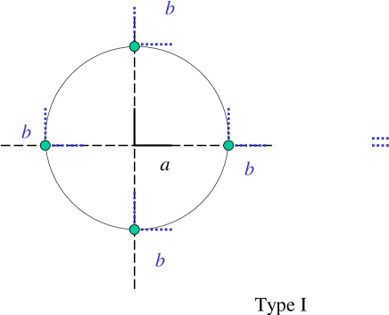
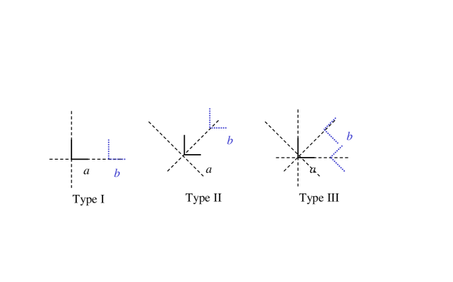
Figure 2: Type I configuration with a given separation angle $\beta$. Relative to a fixed L-shaped interferometer $a$, the second one must be placed on two great circles shown with long-dashed lines (left panel). We also have four equivalent detector orientations due to mod-$90^{\circ}$ freedom as shown in the right panel.

Figure 3: Position and orientation of the second detector $b$ relative to the fixed first one $a$. The long dashed lines are great circles passing the first one $a$.

For type I, the solutions of the two angles $\sigma_{1,2}$ are $\sigma_{1}=\sigma_{2}=45^{\circ}$ (mod $90^{\circ}$) and the detector $b$ must be placed on one of the two great circles passing through the detector $a$, parallel to one of the two arms as shown in Figure 3. For a given separation $\beta$, there are four points for the cites of the detector $b$. At each point we have four equivalent orientations as shown in the right panel of Figure 3. This is because response of an L-shaped detector has mod-$90^{\circ}$ effective equivalence. After all, for a given separation $\beta$, there are totally $4\times 4=16$ possible configurations of detector $b$.

For type II, the second detector must reside in two great circles parallel or perpendicular to the bisecting line of each detector, as shown in Figure 3. As in the case of type I, with a given separation $\beta$ we have totally 16 candidates for detector $b$. At the limits $\beta\to 0^{\circ}$ and $\beta\to 180^{\circ}$, there are no essential differences between types I and II.

Similarly, the type III configuration is realized by placing the second detector on one of the four great circles defined for types I and II, with rotating $45^{\circ}$ relative to the first detector (see Fig. 3). In this case we have $8\times 4=32$ possible configurations for detector $b$. Note that the sensitivity to the $V$-mode is automatically switched off for the type I and II configurations and is conversely maximized for the type III configuration. This is because the function $\gamma_{V}$ is proportional to $\sin(4\Delta)$.

III.5 Basic properties of functions $\Theta_{i}$

In this subsection, specifically focusing on the detectors on the Earth with radius $R_{\rm E}$=6400km, we study basic properties of the three functions $\Theta_{1}$, $\Theta_{2}$ and $\Theta_{3}$ in some details. Note that in general, for a sphere with radius $R_{\rm s}$, there is one characteristic frequency $c/R_{\rm s}$ and our results for the Earth at frequency $f$ can be rescaled to those for the sphere with scaled frequency $(R_{\rm E}/R_{\rm s})\,f$ . Hence, the result presented here may be interpreted as the one for an arbitrary sphere, including multiple detectors placed on the Moon.

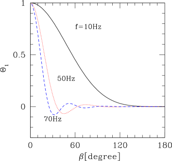
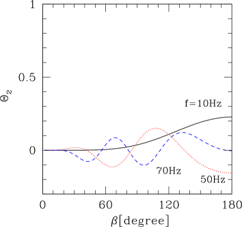
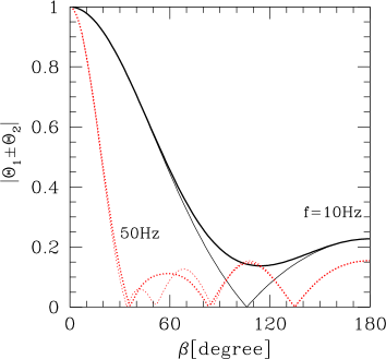
Figure 4: The functions $\Theta_{1}(f,\beta)$ and $\Theta_{2}(f,\beta)$ for detectors on the Earth at frequencies $f=10$Hz, 50Hz and 70Hz.

Figure 5: The optimal combinations $|\Theta_{1}(f,\beta)+\Theta_{1}(f,\beta)|$ (type II: thick lines) and $|\Theta_{1}(f,\beta)-\Theta_{1}(f,\beta)|$ (type I: thin lines) for detectors on the Earth at frequencies $f=10$Hz and 50Hz.

In left panel of Figure 5, the function $\Theta_{1}(f,\beta)$ is plotted against the angle parameter $\beta$ at specific frequencies $f=10$, 50 and 70Hz. As shown in Sec. III.3, we have $\Theta_{1}=1$ at $\beta=0^{\circ}$ that is the maximum value for $\gamma_{I}$ for given frequency $f$. At frequency $f\geq 10$Hz relevant for ground-based detectors, the function $|\Theta_{1}|$ becomes very small for a separation angle $\beta\gtrsim 90^{\circ}$, and we identically have $\Theta_{1}=0$ at antipodal configuration $\beta=180^{\circ}$. In right panel of Figure 5, the shape of the second function $\Theta_{2}(f,\beta)$ is shown. As discussed in Sec. III.3, the function $\Theta_{2}$ becomes vanishing at $\beta=0^{\circ}$. This function exhibits an oscillatory behavior in the range $0^{\circ}\leq\beta\leq 180^{\circ}$, and the number of its nodes is approximately proportional to $fR_{\rm E}$ (see appendix A).

In Figure 5, we plot the overlap function $|\gamma_{I}|$ for two optimal configurations, types I and II, at specific frequencies $10$ and $50$Hz. The thin lines are for the type I with $|\gamma_{I}|=|\Theta_{1}-\Theta_{2}|$, while the thick lines are for the type II with $|\gamma_{I}|=|\Theta_{1}+\Theta_{2}|$. For angles close to $\beta=0^{\circ}$ and $180^{\circ}$, two lines are almost identical. This is because only one component is dominant there, that is, $|\Theta_{1}|\gg|\Theta_{2}|$ at $\beta\sim 0^{\circ}$, and $|\Theta_{2}|\gg|\Theta_{1}|$ at $\beta\sim 180^{\circ}$. Two components have comparable magnitude at $\beta\sim 120^{\circ}$ for $f=10$Hz and at $\beta\sim 60^{\circ}$ for $f=50$Hz. As shown with the curves for $f=50$Hz, both types I and II have chance to give the maximum value of $|\gamma_{I}|$ for given $(f,\beta)$, depending on the relative signs of $\Theta_{1}$ and $\Theta_{2}$.

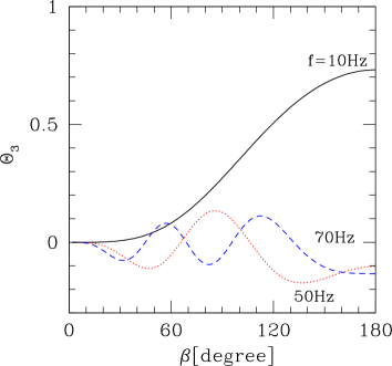
Figure 6: The function $\Theta_{3}(f,\beta)$ for detectors on the Earth at frequencies $f=10$Hz, 50Hz and 70Hz.

Figure 7: Values of $\beta_{\rm max}$ for detectors on the Earth as a function of frequency. While vertical lines are shown due to a software reason, there are discontinuities from $\beta_{\rm max}<180^{\circ}$ to $\beta_{\rm max}=180^{\circ}$.

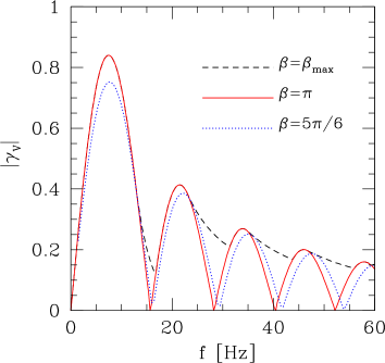
Figure 8: The function $|\gamma_{V}|$ for detectors on the Earth with type III configuration. The solid curve (dotted curve) is the result with $\beta=\pi$ ($\beta=5\pi/6$). The dashed line is result with $\beta_{max}$ for which the function $|\gamma_{V}|$ becomes maximum with given frequency $f$.

Next, in Figure 7, the function $\Theta_{3}$ for the $V$-mode is plotted. Note that we have $|\gamma_{V}|=|\Theta_{3}|$ for the type III configuration. As in the case for $\Theta_{2}$, the oscillating profiles have a number of nodes approximately proportional to $fR_{\rm E}$. For given frequency $f$, we define the separation angle $\beta_{\rm max}$ that maximizes the function $|\Theta_{3}|$ in the range $\beta\in[0^{\circ},\,\,180^{\circ}]$. In contrast to the simple results for the $I$-mode with $\max\gamma_{I}(f,\beta)=\Theta_{1}(f,\beta=0^{\circ})=1$, the angle $\beta_{\rm max}$ defined for the $V$-mode is slightly complicated and it does depend on the frequency $f$. Figure 7 shows the angle $\beta_{max}$ in unit of radian, plotted against the frequency. The frequency dependence in the range $0<f<16.7$Hz can be understood with the following three steps:

(i)

As commented earlier, we have $\partial_{\beta}\Theta_{3}(f,\beta=180^{\circ})=0$ representing that the end point $\beta=180^{\circ}$ is generally an extreme. At low frequency regime, the oscillating feature of $\Theta_{3}$ is relatively simple (see Fig. 7), and the end point $\Theta_{3}(f,\beta=180^{\circ})$ is the global maxima. We find $\beta_{\rm max}=180^{\circ}$ for $f\leq 12.8$Hz.

(ii)

At $f=12.8$Hz, the end point $\beta=180^{\circ}$ becomes an inflection point with $\partial^{2}_{\beta}\Theta_{3}(f,\beta=180^{\circ})=0$. Then, for $f>12.8$Hz, there appears a local maxima for $\Theta_{3}$ at $\beta<180^{\circ}$ that determines the separation angle $\beta_{\rm max}$, as in Figure 7. Meanwhile the end point $\Theta_{3}(f,\beta=180^{\circ})$ is now a local minimum. With increasing $f$ it decreases and crosses 0 at $f=15.7$Hz.

(iii)

The local maxima $\Theta_{3}(f,\beta_{\rm max})$ at $\beta_{\rm max}<180^{\circ}$ coincides with $-\Theta_{3}(f,\beta=180^{\circ})$ ($>0$) at $f=16.7$Hz, and the separation angle $\beta_{\rm max}$ shows a discontinuous transition up to $\beta_{\rm max}=180^{\circ}$ at $f=16.7$Hz.

We can observe similar cycles for the angle $\beta_{\rm max}$ at $f>16.7$Hz. The frequency dependent angle $\beta_{\rm max}$ should be regarded as the optimal separation for narrow band detection for the $V$-mode signal. In Figure 8, we show the maximum value $|\Theta_{3}(f,\beta_{\rm max})|$ as well as $|\Theta_{3}(f,\beta=180^{\circ})|$ and $|\Theta_{3}(f,\beta=150^{\circ})|$. The choice $\beta=150^{\circ}$ is just for an example. The first two curves coincide at some frequency bands (as shown in Fig. 7 for $\beta_{\rm max}$), while the example $|\Theta_{3}(f,\beta=150^{\circ})|$ contacts with the dashed curve for maximum value $|\Theta_{3}(f,\beta_{\rm max}|$ only at specific discrete frequencies. In the two dimensional region with $0^{\circ}\leq\beta\leq 180^{\circ}$ and $f\geq 0$, the global maximum for $\Theta_{3}$ is

$$-\frac{5}{32}(2\cos 2-5\sin 2)=0.84,$$ (35)

which appear at $\beta=180^{\circ}$ and $f=c/2\pi R_{\rm E}=7.5$Hz for detectors on the Earth with $R_{\rm E}=6400$km. In general, the function $\Theta_{3}$ is maximized at antipodal configuration ($\beta=180^{\circ}$) with $f={c}/{2\pi R_{\rm s}}$, or equivalently $y=2$ due to the scaling commented in the beginning of this subsection. Although, for practical purpose to detect the $V$-mode signal, the broad-band analysis with multiple detectors is essential, which we will discuss in next section, it is clear from Figure 8 that the separation $\beta=180^{\circ}$ seems the best choice for detectors, whose bandwidths are much larger than the individual wiggle structure in this figure.

III.6 Overlap functions for specific pairs of detectors

Now, we analyze the geometry of ten pairs made from the five detectors listed in Table 1. In this paper, we do not consider the co-located and co-aligned pair of detectors, such as two interferometers (4km+2km) at LIGO-Hanford. Co-located and co-aligned detectors are possibly contaminated by the measurement noises which are statistically correlated with each other, making the detection of stochastic signals difficult.

Let us first examine how well the pairs of existing or planned interferometers are suitable for $I$- and $V$-mode detection by comparing the angle parameters with those of the optimal configuration discussed in Sec. III.4. In left panel of Figure 9, we plot the combination $(\cos(4\delta),\cos(4\Delta))$. ¿From this plot, the AL and AH pairs are found to be very close to the type I and type II configurations, respectively. Except for these, however, there are no other noticeable pairs. Turn to next consider a large separation angle $\beta\sim 180^{\circ}$, where the parameter $\delta$ becomes unimportant and the correlation signal can be approximately described by

$$C_{ab}\simeq\frac{8\pi}{5}\left[\Theta_{2}(y,\beta)\cos(4\Delta)+\Theta_{3}(y,\beta)\sin(4\Delta)\right].$$ (36)

Thus, in this case, the angle parameters $\beta$ and $\Delta$ now play an important role. Since the regime $\beta\gtrsim 90^{\circ}$ is preferable for the $V$-mode detection, we next plot the combination $(\beta,\cos(4\Delta))$ in right panel of Figure 9. Among various pairs of detectors, the CL pair realizes nearly ideal angle ($\sin(4\Delta)=-1$), although the separation angle of CL pair is intermediate, i.e., $\beta=99.2^{\circ}$. Other interesting pairs for the $V$ mode with relatively large $|\sin(4\Delta)|$ are AV ($\sin(4\Delta)=-0.89$) and CH ($\sin(4\Delta)=0.98$). The HL pair has $\sin(4\Delta)=-0.93$, but its separation is small, $\beta=27.2^{\circ}$, where the amplitude $\Theta_{3}(y,\beta)$ is relatively small.

Based on these considerations, in Figure 10, we compile the overlap functions ($\gamma_{I},\gamma_{V}$) for the ten pairs of detectors. There is characteristic frequency-width, $\Delta f\propto(\sin\beta/2)^{-1}$, determined by the arrival-time difference of gravitational waves between two cites. The frequency interval is largest for the HL pair. For high frequencies, the peaks for the functions $\gamma_{I}$ and $\gamma_{V}$ have 1/4-cycle phase difference, as discussed in appendix A. The AH pair is almost insensitive to the $V$ mode, because it is close to the type II configuration. The situation is similar for the AL pair. Note that the CL and AV pairs have relatively good sensitivity to the $V$ mode, as anticipated from the angular parameters.

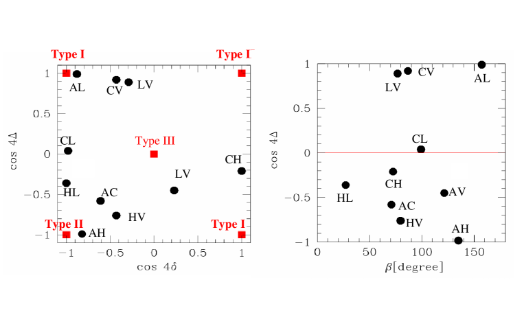
Figure 9: Left: Distribution of the combinations $(\cos 4\delta,\cos 4\Delta)$ for ten detector pairs shown in Table 2. Points for three types of configurations are also given with squares. Right: Distribution of the combinations $(\beta,\cos(4\Delta))$ for ten pairs shown in Table 2. At relatively large $\beta$ the sensitivity to the $V$-mode is roughly proportional to $\sin(4\Delta)$.

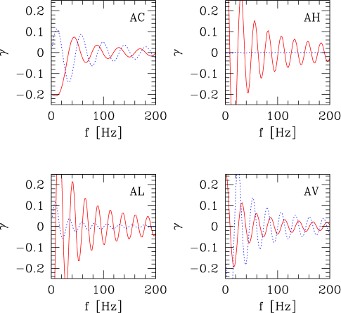
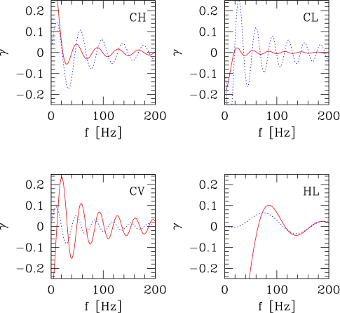
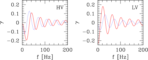
Figure 10: Overlap functions for specific pair of detector made from the five detectors, A, C, H, L and V. The solid lines are for $\gamma_{I}$ and the dotted lines for $\gamma_{V}$.

IV Broadband signal analysis

IV.1 Preliminary

So far, we have only dealt with the correlation signal of gravitational-wave backgrounds. In practice, the signal is contaminated by detector’s noises, and thus the broadband signal analysis is essential ingredient for detection of background signals with high signal-to-noise ratio.

We model the data stream $s_{a}$ of a detector $a$ by a summation of gravitational-wave signal $H_{a}$ and detector noise $n_{a}$,

$$s_{a}=H_{a}+n_{a}.$$ (37)

Throughout this paper, we assume that the noise of detector, $n_{a}$, obeys stationary and random processes and the noise correlation between any pair of detectors can be safely neglected. Then, covariance of the detector noises can be expressed as

$$\left\langle n_{a}(f)n_{b}(f^{\prime})^{*}\right\rangle=\frac{1}{2}\delta_{ab}\delta_{\rm D}(f-f^{\prime})N_{a}(f),$$ (38)

where $N_{a}$ is the noise spectral density for detector $a$.

To estimate the sensitivity of each pair of detectors, let us consider the simple case with correlation $C_{ab}(f)$ of two detectors $a$ and $b$. As it has been shown in the literature, the total signal-to-noise ratio (SNR) is given by Flanagan:1993ix ; Allen:1997ad (see also appendix B)

$$\mathrm{SNR}^{2} = \left(\frac{16\pi}{5}\right)^{2}T_{\rm obs}\left[2\int_{0}^{\infty}df\frac{(\gamma_{I}I+\gamma_{V}V)^{2}}{{\cal N}_{ab}(f)}\right]$$ (39)

$$= \left(\frac{3H_{0}^{2}}{10\pi^{2}}\right)^{2}T_{\rm obs}\left[2\int_{0}^{\infty}df\frac{\Omega_{\rm GW}(f)^{2}(\gamma_{I}+\gamma_{V}\Pi)^{2}}{f^{6}{\cal N}_{ab}(f)}\right]$$

with the quantity ${\cal N}_{ab}$ defined by ${\cal N}_{ab}\equiv N_{a}(f)N_{b}(f)$. This is the result obtained in the weak-signal limit $I(f)\ll N_{\{a,b\}}(f)$. Note that the above formula just represents the SNR for the total amplitude of the background signals, and it does not imply the SNR for a pure $I$- or $V$-mode signal. The separation of $I$- and $V$-modes will be discussed in next section.

For quantitative evaluation of SNRs, we need an explicit form of the noise spectral density. In the following, we use the fitting form of the noise spectra for advanced LIGO detector, $N_{\rm ligo}$. Assuming that all the detectors have identical noise spectra with $N_{\rm ligo}$, signal-to-noise ratios of stochastic signals are estimated. Based on Ref.adv , the analytical fit of the noise spectrum $N_{\rm ligo}$ is given by

$$N_{\rm ligo}(f)=\left\{\begin{array}[]{lcl}{\displaystyle 10^{-44}\left(\frac{f}{\rm 10Hz}\right)^{-4}+10^{-47.25}\left(\frac{f}{\rm 100Hz}\right)^{-1.7}}{\rm Hz^{-1}}&{\rm for}&10{\rm Hz}\leq f\leq 240{\rm Hz},\\ {\displaystyle 10^{-46}\left(\frac{f}{\rm 1000Hz}\right)^{3}}{\rm Hz^{-1}}&{\rm for}&240{\rm Hz}\leq f\leq 3000{\rm Hz},\\ \infty&{}\hfil&{\rm otherwise}.\end{array}\right.$$ (40)

The expression (39) implies that the weight function for SNR per logarithmic frequency interval $d\ln f$ is proportional to $(N(f)f^{5/2})^{-1}$ for flat input $\Omega_{\rm GW}(f)(\gamma_{I}+\gamma_{V}\Pi)={\rm const}$. In Figure 11, using the analytic form of the noise spectrum, we plot the weight function. It becomes maximum around $\sim 50$Hz with its bandwidth $\sim 100$Hz. Note that the shape of the weight function for stochastic signals is close to the one for the signals produced by binary neutron stars, in which case the detectable distance, as the integral of weight function, is roughly proportional to

$$\left[\int_{0}^{\infty}d\ln f\frac{1}{f^{4/3}N(f)}\right]^{1/2}.$$ (41)

The next-generation detectors are primarily designed to have the good sensitivity to a chirping signal of binary neutron stars, and they are planned to achieve the similar performance for detecting these binaries. In this sense, our assumption that all the detectors have identical noise spectrum with advanced LIGO is reasonable.

Finally, as a reference, we present the SNR for coincident detectors ($\gamma_{I,ab}=1,\gamma_{V,ab}=0$):

$$\mathrm{SNR}_{0}=4.8\left(\frac{T_{\rm obs}}{3\rm yr}\right)^{1/2}\left(\frac{\Omega_{\rm GW}h_{70}^{2}}{10^{-9}}\right).$$ (42)

This value will be frequently referred, as a baseline of the SNR for various situations considered below.

Figure 11: The weight function $(N(f)f^{5/2})$ for advanced LIGO.

IV.2 Signal-to-noise ratios for pair of detector

The total SNR (39) depends strongly on model parameters of the background, including the polarization degree $\Pi$. In order to present our numerical results concisely, we use the normalized form

$$Q\equiv\frac{\rm SNR}{\rm SNR_{0}}.$$ (43)

To characterize sensitivity of each pair to $I$- or $V$-mode signal, based on the above equation, we respectively define $Q_{I}$ and $Q_{V}$ by replacing $\{I,\,\,V\}$ in the expression of SNR with $\rho_{c}/(4\pi^{2}f^{3})\{\Omega_{\rm GW},\,\,0\}$ and $\rho_{c}/(4\pi^{2}f^{3})\{0,\,\,\Omega_{\rm GW}\}$. These normalized SNRs $Q_{I}$ and $Q_{V}$ can be regarded as a rms value of overlap functions with the weight function $(f^{5/2}N(f))^{-1}$.

In Figure 13, we present the normalized SNR for the optimal geometry, i.e., types I, II and III configurations (short-dashed, long-dashed and solid lines, respectively). One noticeable point is that a widely separated ($\beta\sim 180^{\circ}$) pair is powerful to search for the $V$ mode. At $\beta=180^{\circ}$, we find the following asymptotic relations

$$\gamma_{I}\sim-\frac{5}{2}\cos(4\Delta)\frac{\sin y}{y},\quad\gamma_{V}\sim\frac{5}{2}\sin(4\Delta)\frac{\cos y}{y}$$ (44)

with $y=4\pi Rf/c$. For detectors on the Earth, the characteristic frequency interval is $c/2R_{\rm E}\sim 20$Hz, which is enough inside the bandwidth of advance LIGO, $\Delta f\sim 100$Hz. As a result, the oscillation of the overlap functions are averaged out and the normalized SNRs $Q_{I}$ and $Q_{V}$ give a similar output for optimal configurations (types I-III) at $\beta=180^{\circ}$.

In Figure 13 and Table 3, we show the normalized SNRs for pairs made from the five interferometers in Table 1. To reduce the contribution from the $I$-mode signal, pairs that have been regarded as disadvantageous for constraining $\Omega_{\rm GW}$, can now play important roles for measuring the $V$ mode, according to equation (36). The HL pair with $\cos(4\delta)\sim 1$ and $\sin(4\Delta)\sim 0.93$ realizes nearly maximum values simultaneously for ${Q}_{I,ab}$ and ${Q}_{V,ab}$, at its separation $\beta=27.2^{\circ}$. This is because ${Q}_{I,ab}$ is mainly determined by the angle $\delta$ at a small $\beta$, while ${Q}_{V,ab}$ depends only on $\Delta$. This pair has the largest $Q_{I}$ among ten pairs of detectors. In contrast, the CL pair has good sensitivity to $V$, although it is relatively insensitive to the $I$ mode, because of $\sin(4\Delta)\sim 1$ and $|\cos(4\Delta)|=0.04$. Indeed, the orientation of the LCGT detector is only $1.2^{\circ}$ different from the optimal direction ($\cos(4\Delta)=0$) with respect to the LIGO-Livingston cite. As other interesting pairs, the AH pair is almost insensitive to the $V$ mode with $\sin(4\Delta)=-0.007$ (nearly type II configuration with LIGO-Hanford). The AV pair has a large $Q_{V}$ with $|\sin(4\Delta)|=0.89$, but its $Q_{I}$ is much larger than that of the CL pair.

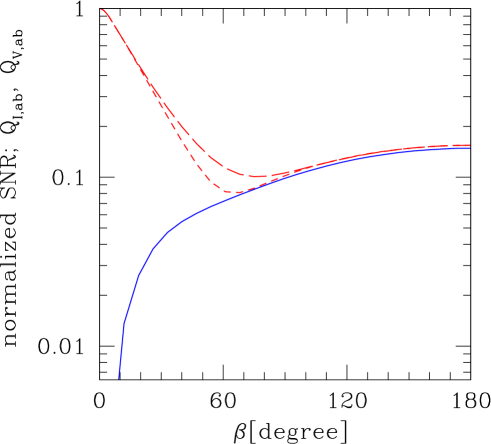
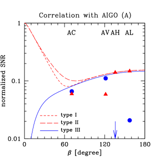
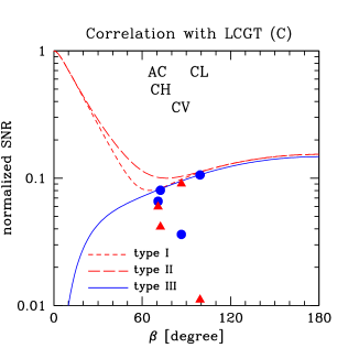
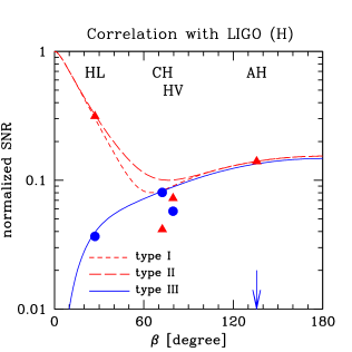
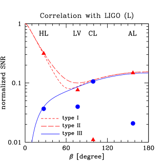
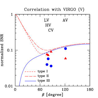
Figure 12: Normalized signal to noise ratios (${Q}_{I,ab}$ and ${Q}_{V,ab}$) with optimal configurations for the $I$-mode (short dashed curve: type I, long dashed curve: type II) and for the $V$-mode (solid curve: type III with setting $\Pi=1$ for illustrative purpose). We use the noise curve for the advanced LIGO.

Figure 13: The normalized SNRs $Q_{I}$ (circles) and $Q_{V}$ (triangles) for detector pairs.

	A	C	H	L	V
A	$*$	$0.060$	$0.14$	$0.15$	$0.059$
C	$0.07$	$*$	$0.042$	$0.011$	$0.091$
H	$0.0009$	$0.081$	$*$	$0.32$	$0.073$
L	$0.021$	$0.11$	$0.037$	$*$	$0.077$
V	$0.11$	$0.036$	$0.058$	$0.040$	$*$

Table 3: Normalized SNRs $Q_{I}$ (upper-right) and $Q_{V}$ (lower-left).

IV.3 Antipodal detectors

So far, we have studied pairs of detectors on the Earth, strictly keeping the radius of sphere $R_{\rm E}=6400$km, for which the antipodal type III configuration is turned out to be optimal to realize the largest SNR $Q_{V}$. Here, we discuss to what extent one can improve the sensitivity to the $V$ mode by varying the radius of sphere.

In Figure 15, we plot the broadband sensitivities $Q_{I}$ and $Q_{V}$ for antipodal detectors as functions of the radius of sphere, $R$. Note that the noise spectrum is fixed to $N_{\rm ligo}(f)$ as before. Here, we put $\cos(4\Delta)=1$ for $Q_{I}$ and $\sin(4\Delta)=1$ for $Q_{V}$. While the value $Q_{I}$ is maximized at $R=0$ and we obtain $Q_{I}=1$ and $Q_{V}=0$, the maximum value of $Q_{V}$ is achieved when $R=600$km, leading to $Q_{V}=0.64$. It is interesting to note that at $R\sim 1700$km corresponding to the radius of the Moon, we still obtain rather larger value, $Q_{V}=0.45$.

In Figure 15, the overlap functions for three representative cases are plotted: $R=600$, $1700$ and $6400$km. As we commented earlier, the overlap functions for any radius can be rescaled and become identical if we plot the functions against the rescaled variable, $y\propto fR$. Further, for the configuration examined in Figure 15, the relations $\gamma_{I}(0)=-1$ and $\gamma_{V}(0)=0$ strictly hold. In those situations, the shape of the noise spectrum shown in Figure 11 is the key to determine the best value for $Q_{V}$ and the overlap function $\gamma_{V}$ for $R\sim 600$km eventually becomes the best shape to achieve the maximum value of $Q_{V}=0.64$. Also, it turned out that the sensitivity for the Moon becomes about three times larger than that for the Earth, $Q_{V}=0.15$ (see appendix D for comments on detectors on the Moon).

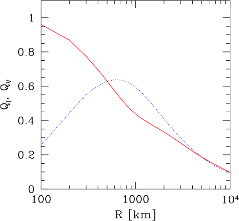
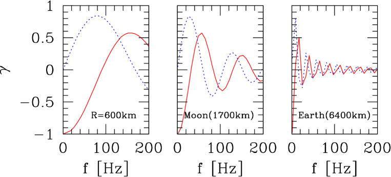
Figure 14: The normalized SNR for antipodal configuration with radius $R$. Advanced LIGO noise curve is used.

Figure 15: Overlap functions for antipodal detector pairs (solid curves: $\gamma_{I}$, dotted curves: $\gamma_{V}$).

V Separation

As discussed so far, a simple analysis with correlation signal $C_{ab}$ of two detectors allows us to detect a mixture of $I$- and $V$-mode signals, but we cannot extract each of them separately. In order to disentangle these two signals, in this section, we discuss the problem of the $I$- and $V$-mode separation considered in Ref.Seto:2007tn . After describing the simplest case using a set of four detectors in Sec.V.1, we generalize it to the multiple-detector case in Sec. V.2, and present a statistical framework to achieve the optimal sensitivity. Based on these theoretical backgrounds, in Sec. V.3, the correlation analysis with network of ground-based detectors are examined and the optimal values of SNR are derived for each $I$ and $V$ mode.

V.1 Analysis with two correlation signals

Let us begin by considering the simplest case that two pairs of interferometers $(a,b)$ and $(c,d)$ are available. We write down their correlation signals as

$$C_{ab}(f)=\frac{8\pi}{5}\{\gamma_{I,ab}(f)I(f)+\gamma_{V,ab}(f)V(f)\},\quad C_{cd}(f)=\frac{8\pi}{5}\{\gamma_{I,cd}(f)I(f)+\gamma_{V,cd}(f)V(f)\}.$$ (45)

Making their linear combination, $I$ or $V$ mode can be removed, and a pure $V$ or $I$ mode is separately extracted. Except for trivial scaling, the unique choices are

$${\gamma_{V,ab}C_{cd}-\gamma_{V,cd}C_{ab}}=\frac{8\pi}{5}I{(\gamma_{I,cd}\gamma_{V,ab}-\gamma_{I,ab}\gamma_{V,cd})},\quad{\gamma_{I,ab}C_{cd}-\gamma_{I,cd}C_{ab}}=\frac{8\pi}{5}V{(\gamma_{V,cd}\gamma_{I,ab}-\gamma_{V,ab}\gamma_{I,cd})}.$$ (46)

Meanwhile, the noise spectra for these combinations are proportional to

$${\gamma_{V,ab}^{2}{\cal N}_{cd}+\gamma_{V,cd}^{2}{\cal N}_{ab}},\quad{\gamma_{I,ab}^{2}{\cal N}_{cd}+\gamma_{I,cd}^{2}{\cal N}_{ab}},$$ (47)

where quantity ${\cal N}_{ab}$ indicates the product of noise spectra, ${\cal N}_{ab}=N_{a}(f)N_{b}(f)$. Taking account of proportional factors, the broadband signal-to-noise ratio for a pure $I$ or $V$ mode becomes

$$\mathrm{SNR}_{I}^{2} = \left(\frac{16\pi}{5}\right)^{2}T_{\rm obs}\left[2\int_{0}^{\infty}df\frac{I^{2}(\gamma_{V,cd}\gamma_{I,ab}-\gamma_{V,ab}\gamma_{I,cd})^{2}}{(\gamma_{V,ab}^{2}{\cal N}_{cd}+\gamma_{V,cd}^{2}{\cal N}_{ab})}\right],$$ (48)

$$\mathrm{SNR}_{V}^{2} = \left(\frac{16\pi}{5}\right)^{2}T_{\rm obs}\left[2\int_{0}^{\infty}df\frac{V^{2}(\gamma_{V,cd}\gamma_{I,ab}-\gamma_{V,ab}\gamma_{I,cd})^{2}}{(\gamma_{V,ab}^{2}{\cal N}_{cd}+\gamma_{V,cd}^{2}{\cal N}_{ab})}\right].$$ (49)

For detectors with identical noise spectra with ${\cal N}(f)=N(f)^{2}$, the compiled overlap functions are defined as

$$\Gamma_{I,ab:cd}\equiv\frac{\gamma_{I,cd}\gamma_{V,ab}-\gamma_{I,ab}\gamma_{V,cd}}{[\gamma_{V,ab}^{2}+\gamma_{V,cd}^{2}]^{1/2}},\quad\Gamma_{V,ab:cd}\equiv\frac{\gamma_{V,cd}\gamma_{I,ab}-\gamma_{V,ab}\gamma_{I,cd}}{[\gamma_{I,ab}^{2}+\gamma_{I,cd}^{2}]^{1/2}}.$$ (50)

With these functions, the broadband SNRs for the separated two modes can be estimated from equation (39) just replacing the term $\gamma_{I}I+\gamma_{V}V$ with $\Gamma_{I,ab:cd}I$ and $\Gamma_{V,ab:cd}V$. In this sense, the complied overlap functions represent the sensitivities to the $I$ and $V$ modes after the separation.

In Figure 16, as a specific example for the mode separation, we consider the HL and CL pairs and plot the compiled overlap function, as well as the overlap functions for each pair. Although the shapes of the functions $\Gamma_{ab:cd}$ are very complicated, resultant values of the normalized SNR estimated from equations (48) and (49) are $0.11$ for the $V$ mode and $0.31$ for the $I$ mode, which are very close to the values presented in Sec. IV.2 (${Q}_{V}=0.11$ for CL, ${Q}_{I}=0.32$ for HL). Note also that for other combinations, the $I$ and $V$-mode separation can be performed with nominal changes to the naively expected sensitivities ${Q}_{\{I,V\},ab}$. This will be discussed in details in Sec. V.3.

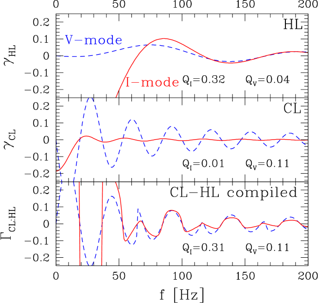
Figure 16: Overlap functions for the unpolarized $I$ mode (dashed curves), and the circularly polarized $V$ mode (solid curves). The upper panel shows the results for the Hanford-Livingston (HL) pair. The middle one is results for the LCGT-Livingston (CL) pair. The normalized SNRs ${\it S}_{I,V}$ (with the adv LIGO noise spectrum) are also presented. The bottom one show the compiled functions $\Gamma_{I,V}$ (Eq.(50)) made from both pairs.

V.2 Analysis with multiple data set

Next consider the generalization of the previous analysis to the cases with multiple data set. For a network of $n$ detectors, we can make totally $n_{t}=n(n-1)/2$ independent correlation signals

$$C_{i}=\frac{8\pi}{5}(\gamma_{Ii}\,I+\gamma_{Vi}\,V)$$ (51)

with $i=1,..,n_{t}$. Here, we use the single suffix $i$ to represent a detector pair for which we have assigned two suffixes so far, such as $ab$ in equation (45). For the number of detectors with $n>2$, the number of output signals becomes $n_{t}>3$, and this implies that we must deal with the over-determined problem in order to separate a mixture of $I$- and $V$-modes, because the number of observables exceeds the number of target parameters, $I$ and $V$. In what follows, we will discuss the signal-to-noise ratios expected from the optimal data analysis.

Let us examine a straightforward extension of the analysis in previous subsection. Provided the original data set of correlation signals, $\{C_{i}\}$, obtained from all possible pairs of detectors, we can make the linear combinations, $D_{Ii}$ and $D_{Vi}$, which respectively eliminate the variable $V$ and $I$:

$$D_{Ii}=d_{Ii}I,~{}~{}~{}D_{Vi}=d_{Vi}V,$$ (52)

where $d_{Ii}$ and $d_{Vi}$ denote some numerical coefficients, appropriately chosen for removing the contribution from $V$ and $I$, respectively. Note that the number of independent combinations labeled as $i$ is $n_{t}-1$ . The associated covariance matrices for intrinsic noises, ${\cal M}^{-1}_{Iij}$ and ${\cal M}^{-1}_{Vij}$, are expressed in terms of the quantities, $\gamma_{Ii}$, $\gamma_{Vi}$ and ${\cal N}_{i}$ (noise spectra). Then, the resultant total SNRs for the optimal combinations of data sets $\{D_{Ii},D_{Vi}\}$ are

$$\mathrm{SNR}_{I}^{2}\propto d_{Ii}{\cal M}^{-1}d_{Ij},\quad\mathrm{SNR}_{V}^{2}\propto d_{Vi}{\cal M}^{-1}_{Vij}d_{Vj}.$$ (53)

For $n_{t}=n=3$, the above expressions can be recast in a rather simple form:

$$\mathrm{SNR}_{I}^{2} \propto I^{2}\left[\left(\sum_{i}^{3}\frac{\gamma_{Ii}^{2}}{{\cal N}_{i}}\right)\left(\sum_{i}^{3}\frac{\gamma_{Vi}^{2}}{{\cal N}_{i}}\right)-\left(\sum_{i}^{3}\frac{\gamma_{Ii}\gamma_{Vi}}{{\cal N}_{i}}\right)^{2}\right]\left(\sum_{i}^{3}\frac{\gamma_{Vi}^{2}}{{\cal N}_{i}}\right)^{-1},$$ (54)

$$\mathrm{SNR}_{V}^{2} \propto V^{2}\left[\left(\sum_{i}^{3}\frac{\gamma_{Ii}^{2}}{{\cal N}_{i}}\right)\left(\sum_{i}^{3}\frac{\gamma_{Vi}^{2}}{{\cal N}_{i}}\right)-\left(\sum_{i}^{3}\frac{\gamma_{Ii}\gamma_{Vi}}{{\cal N}_{i}}\right)^{2}\right]\left(\sum_{i}^{3}\frac{\gamma_{Ii}^{2}}{{\cal N}_{i}}\right)^{-1}.$$ (55)

Equations (54) and (55) are symmetric with respect to the suffix $i$ and they do not depend on the specific choice of the data sets $\{D_{Ii},D_{Vi}\}$. Self-consistently, the above expressions recover the previous results, (48) and (49), if we set $\gamma_{I3}$ and $\gamma_{V3}$ to zero. Indeed, the symmetric expressions (54) and (55) for $n_{t}=3$ generally hold for the cases with $n_{t}>3$ and we will use these forms to estimate the SNRs for optimal combination of five ground-based detectors. In appendix C, a brief sketch to derive the symmetric expressions for the $n_{t}>3$ cases is presented. Multiplying the factor $2(16\pi/5)^{2}df$ and integrating over entire frequency range, the narrow band SNRs (54) and (55) can be generalized to the broadband SNRs

$$\mathrm{SNR}_{I}^{2} = 2\left(\frac{16\pi}{5}\right)^{2}T_{\rm obs}\int_{0}^{\infty}dfI^{2}\left[\left(\sum_{i}^{n_{t}}\frac{\gamma_{Ii}^{2}}{{\cal N}_{i}}\right)\left(\sum_{i}^{n_{t}}\frac{\gamma_{Vi}^{2}}{{\cal N}_{i}}\right)-\left(\sum_{i}^{n_{t}}\frac{\gamma_{Ii}\gamma_{Vi}}{{\cal N}_{i}}\right)^{2}\right]\left(\sum_{i}^{n_{t}}\frac{\gamma_{Vi}^{2}}{{\cal N}_{i}}\right)^{-1},$$ (56)

$$\mathrm{SNR}_{V}^{2} = 2\left(\frac{16\pi}{5}\right)^{2}T_{\rm obs}\int_{0}^{\infty}dfV^{2}\left[\left(\sum_{i}^{n_{t}}\frac{\gamma_{Ii}^{2}}{{\cal N}_{i}}\right)\left(\sum_{i}^{n_{t}}\frac{\gamma_{Vi}^{2}}{{\cal N}_{i}}\right)-\left(\sum_{i}^{n_{t}}\frac{\gamma_{Ii}\gamma_{Vi}}{{\cal N}_{i}}\right)^{2}\right]\left(\sum_{i}^{n_{t}}\frac{\gamma_{Ii}^{2}}{{\cal N}_{i}}\right)^{-1}.$$ (57)

Similar to the one defined in previous subsection, we define the effective overlap functions for detectors with identical noise spectra, which represent the optimal sensitivities to the $I$ and $V$ modes:

$$\Gamma_{{\rm eff},I}\equiv\left(\frac{\sum_{i}^{n_{t}}\gamma_{iI}^{2}\sum_{i}^{n_{t}}\gamma_{iV}^{2}-(\sum_{i}^{n_{t}}\gamma_{iI}\gamma_{iV})^{2}}{\sum_{i}^{n_{t}}\gamma_{iV}^{2}}\right)^{1/2},\quad\Gamma_{{\rm eff},V}\equiv\left(\frac{\sum_{i}^{n_{t}}\gamma_{iI}^{2}\sum_{i}^{n_{t}}\gamma_{iV}^{2}-(\sum_{i}^{n_{t}}\gamma_{iI}\gamma_{iV})^{2}}{\sum_{i}^{n_{t}}\gamma_{iI}^{2}}\right)^{1/2}.$$ (58)

For sensitivity only for the $I$ or $V$ mode, we also define

$$\Gamma_{{\rm eff},I0}=\left(\sum_{i}^{n_{t}}\gamma_{iI}^{2}\right)^{1/2},\quad\Gamma_{{\rm eff},V0}=\left(\sum_{i}^{n_{t}}\gamma_{iV}^{2}\right)^{1/2},$$ (59)

which correspond to the effective overlap function (with identical noise spectrum) for the traditional analysis in the absence of $V$ or $I$ mode. In the following, we use the notation $Q_{I0}$ for the normalized SNR with effective function $\Gamma_{{\rm eff},I0}$. Based on these definitions, the ratio $R$ is given by

$$R=\frac{\sum_{i}^{n_{t}}\gamma_{iI}\gamma_{iV}}{\Gamma_{{\rm eff},I0}\Gamma_{{\rm eff},V0}}.$$ (60)

As increasing the number of detectors, the functions $\Gamma_{{\rm eff},I0}$ and $\Gamma_{{\rm eff},V0}$ monotonically increase. For a large numbers of detectors, however, the numerator $\sum_{i}^{n_{t}}\gamma_{iI}\gamma_{iV}$ can be regarded as a summation of random numbers, and the ratio $R$ is expected to decrease quickly. We will see this numerically in next subsection.

V.3 Optimal SNRs from ground-based network

We are in position to evaluate the broad band SNRs for optimal combination of network of five detectors, A,C,H,L and V. For networks made by three detectors among five detectors, there are ${}_{5}C_{3}=10$ possible networks. In the same way, we can make ${}_{5}C_{4}=5$ networks for combinations of four detectors. Numerical results for detector networks are presented in Table 4. In Figure 17, we also provide the normalized SNRs for various combinations of detectors, showing the overall behaviors against the number of detectors.

network	$Q_{I}$	$Q_{V}$	$Q_{I0}$
ACH	$0.15$	$0.10$	$0.16$
ACL	$0.15$	$0.12$	$0.16$
ACV	$0.11$	$0.16$	$0.12$
AHL	$0.33$	$0.04$	$0.37$
AHV	$0.16$	$0.12$	$0.17$
ALV	$0.16$	$0.11$	$0.18$
CHL	$0.31$	$0.13$	$0.32$
CHV	$0.09$	$0.09$	$0.12$
CLV	$0.12$	$0.11$	$0.12$
HLV	$0.32$	$0.07$	$0.33$
ACHL	$0.38$	$0.15$	$0.38$
ACHV	$0.20$	$0.16$	$0.20$
ACLV	$0.20$	$0.17$	$0.21$
AHLV	$0.39$	$0.14$	$0.39$
CHLV	$0.34$	$0.16$	$0.35$
ACHLV	$0.41$	$0.20$	$0.41$

Table 4: Normalized SNRs $Q_{I}$, $Q_{V}$ and $Q_{I0}$ for network of detectors.

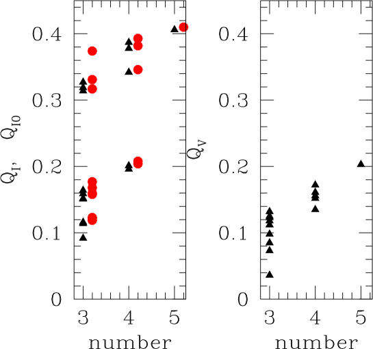
Figure 17: The normalized SNRs $Q_{I}$ (left panel; filled triangles), $Q_{I0}$ (left panel ; open circles), and $Q_{V}$ (right panel; filled triangle). The horizontal axis is the number of detectors. We slightly shift the points for $Q_{I0}$ to the right.

¿From Table 4 and Figure 17, several diagnostic features are summarized:

(i)

To realize a good sensitivity to the $I$ mode, the HL pair has a crucial role. This is due to their small separation. Without the pair, we have at most $\mathrm{SNR}_{I}=0.20$ and $\mathrm{SNR}_{I0}=0.21$. Including the two detectors, the value $\mathrm{SNR}_{I}$ becomes more than 0.3.

(ii)

The combination AHL does not have a good sensitivity to the $V$ mode and we obtain $Q_{V}=0.04$. This is because the orientation of AIGO detector is specialized to achieve the best sensitivity to $I$ mode in combination with LIGO detectors. In fact, they are aligned to have large overlaps (in relation to (i)). Nevertheless, the sensitivity to the $V$ mode can be improved by adding the LCGT or Virgo detector. In contrast, the value $Q_{I0}$ increases only $10\%$ even if we increase the network from AHL to ACHLV.

(iii)

Comparing $\mathrm{SNR}_{I}$ with $\mathrm{SNR}_{I0}$, we deduce a tiny amount of statistical loss for the sensitivity to the $I$ mode, caused by adding a new target parameter, $V$. It is not preferable to get a significant statistical loss by dealing with the circular polarization mode whose fraction is naively expected to be small. But Table 4 indicates that even when the $V$ mode is added as observational targets, detection efficiency for $I$ mode remains almost unchanged. For three-detector networks, the relative loss is largest for CHV and reach about $24$%. Increasing the number of detectors, the maximum loss is reduced to $4$% for four-detector network, and further reduced to $1$% for five-detector network.

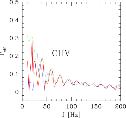
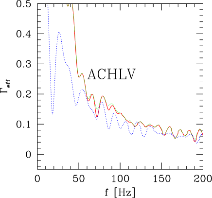
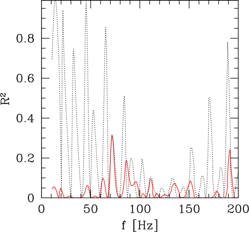
Figure 18: Left: effective overlap functions, $\Gamma_{{\rm eff},I}^{2}$ (solid), $\Gamma_{{\rm eff},I}^{2}$(dotted), and $\Gamma_{{\rm eff},I0}^{2}$ (long-dashed). Right: same as in left panel, but for the network of five detectors. Two curves for $\Gamma_{{\rm eff},I}^{2}$ and $\Gamma_{{\rm eff},I0}^{2}$ are nearly overlapped.

Figure 19: The function $R^{2}$ for the CHV (dotted curve) and the ACHLV networks (solid curve).

To further give a deep insight into the diagnosis (iii), in Figure 19, we plot the effective overlap functions $\Gamma_{{\rm eff},I}$, $\Gamma_{{\rm eff},I0}$ and $\Gamma_{{\rm eff},V}$ for specific networks of CHV (left) and ACHLV (right). For network of CHV, there exists characteristic pattern at $f>40$Hz with period $\Delta f=18$Hz. The main reason of this comes from the fact that all the pairs, CH, CV and HV, have the separation angle $\beta\sim 80^{\circ}$, leading to the frequency $\Delta f=c/(4R_{\rm E}\sin(80^{\circ}/2))\sim 18$Hz. Focusing on the differences between $\Gamma_{{\rm eff},I}$ and $\Gamma_{{\rm eff},I0}$, we find that while the differences are manifest at low-frequency in CHV system, the functions $\Gamma_{{\rm eff},I}$ and $\Gamma_{{\rm eff},I0}$ in ACHLV system become almost identical even at low-frequency. This is clearly quantified if we plot the ratio $R$ defined in equation (60). Figure 19 reveals that the magnitude of the ratio $R$ is significantly reduced for the ACHLV system, suggesting the fact that the statistical loss is negligibly small. In this respect, negligible statistical loss may be another merit for a network with a large number of detectors.

Finally, from numerical results given above and with a help of equation (42), we summarize the signal-to-noise ratios, $\mathrm{SNR}_{I}$ and $\mathrm{SNR}_{Q}$ (not normalized ones) with noise spectrum of advanced LIGO. For the five-detector network, assuming the flat spectra $\Omega_{\rm GW}=\mathrm{const}$ and $\Omega_{\rm GW}\Pi=\mathrm{const}$, we have

$$\mathrm{SNR}_{I}=1.64\left(\frac{\Omega_{\rm GW}h_{70}^{2}}{10^{-9}}\right)\left(\frac{T_{\rm obs}}{3\rm yr}\right)^{-1/2},\quad\mathrm{SNR}_{V}=0.749\left(\frac{\Omega_{\rm GW}h_{70}^{2}\Pi}{10^{-9}}\right)\left(\frac{T_{\rm obs}}{3\rm yr}\right)^{-1/2}.$$ (61)

VI Summary

In this paper we present prospects for measuring the Stokes $V$ parameter of stochastic gravitational wave backgrounds via the correlation analysis. This parameter characterizes the asymmetry of amplitudes of right- and left-handed waves. As the parity transformation interchanges the two polarization modes, it can be regarded as the basic observational measure to probe parity violation. We made detailed analyses for the basic properties of the overlap functions $\gamma_{I}$ and $\gamma_{V}$, especially their dependencies on geometry of detector configurations.

In contrast to studies only for the unpolarized $I$ mode (equivalently, the energy spectrum $\Omega_{\rm GW}$), we need to develop a new statistical framework to deal with rich structures caused by multi-dimensionality of target parameters. We provide an optimal method that will be applicable to various problems of gravitational-wave backgrounds. Based on our new method, we estimated sensitivities of the planned and proposed next-generation interferometers to the $V$ modes. We found that it is important to have a large number of detectors in order to reduce possible effects due to correlation between target parameters.

We would like to thank M. Ando, N. Kanda and M. Ohashi for useful conversations. This work was in part supported by a Grant-in-Aid for Scientific Research from the Japan Society for the Promotion of Science (No. 18740132).

Appendix A Tensorial expansion

In this appendix we present tensorial decompositions of the overlap functions $\gamma_{I,V}$ (see also Ref.Flanagan:1993ix ) defined for pair of detectors $a$ and $b$ at positions ${\mbox{\boldmath${x}$}}_{a}$ and ${\mbox{\boldmath${x}$}}_{b}$. They are expressed as

$$\gamma_{I,ab}(f)=\frac{5}{8\pi}\int_{S^{2}}d\mbox{\boldmath${n}$}\left[\left\{F_{a}^{+}F_{b}^{+*}+F_{a}^{\times}F_{b}^{\times*}\right\}e^{iy\mbox{\boldmath${n}$}\mbox{\boldmath${m}$}}\right],$$ (62)

and

$$\gamma_{V,ab}(f)=\frac{5}{8\pi}\int_{S^{2}}d\mbox{\boldmath${n}$}\left[i\left\{F_{a}^{+}F_{b}^{\times*}-F_{a}^{\times}F_{b}^{+*}\right\}e^{iy\mbox{\boldmath${n}$}\mbox{\boldmath${m}$}}\right],$$ (63)

with ${\mbox{\boldmath${x}$}}_{a}-{\mbox{\boldmath${x}$}}_{b}=D\mbox{\boldmath${m}$}$ ($D$: distance, ${m}$:unit vector) and $y\equiv 2\pi fD/c$. The beam-pattern functions $F_{a}^{P}$ are written by the the polarization tensor ${\mbox{\boldmath${e}$}}^{P}$ and the detector tensor ${\mbox{\boldmath${d}$}}^{a}$ as

$$F_{a}^{P}={\mbox{\boldmath${d}$}}_{a}:{\mbox{\boldmath${e}$}}^{P}(\mbox{\boldmath${n}$})=d_{ij}^{a}e^{P}_{ij}.$$ (64)

Here the detector tensor ${\mbox{\boldmath${d}$}}_{a}$ is given by two orthonormal vectors ${\mbox{\boldmath${u}$}}_{a}$ and ${\mbox{\boldmath${v}$}}_{a}$ as ${\mbox{\boldmath${d}$}}_{a}=({\mbox{\boldmath${u}$}}_{a}\otimes{\mbox{\boldmath${u}$}}_{a}-{\mbox{\boldmath${v}$}}_{a}\otimes{\mbox{\boldmath${v}$}}_{a})/2$. Therefore, the overlap functions are formally written as

$$\gamma_{I}(f)=\Gamma_{I,ijkl}(f)d_{ij}^{a}d_{kl}^{b},~{}~{}~{}\gamma_{V}(f)=\Gamma_{V,ijkl}(f)d_{ij}^{a}d_{kl}^{b}.$$ (65)

In these expressions we defined

$$\Gamma_{I,ijkl}(f)=\frac{5}{8\pi}\int_{S^{2}}d\mbox{\boldmath${n}$}\left[e^{+}_{ij}(\mbox{\boldmath${n}$})e^{+}_{kl}(\mbox{\boldmath${n}$})+e^{\times}_{ij}(\mbox{\boldmath${n}$})e_{kl}^{\times}(\mbox{\boldmath${n}$})\right]e^{iy\mbox{\boldmath${n}$}\mbox{\boldmath${m}$}}$$ (66)

and

$$\Gamma_{V,ijkl}(f)=-\frac{5i}{8\pi}\int_{S^{2}}d\mbox{\boldmath${n}$}\left[e^{+}_{ij}(\mbox{\boldmath${n}$})e^{\times}_{kl}(\mbox{\boldmath${n}$})-e^{\times}_{ij}(\mbox{\boldmath${n}$})e_{kl}^{+}(\mbox{\boldmath${n}$})\right]e^{iy\mbox{\boldmath${n}$}\mbox{\boldmath${m}$}}.$$ (67)

There are apparent symmetries with respect to the subscripts of the tensor $\Gamma_{I,ijkl}$. For example, it is invariant under the replacement $i\leftrightarrow j$ or $(i,j)\leftrightarrow(k,l)$. Furthermore, with using the correspondences $e^{+}_{ij}(-\mbox{\boldmath${n}$})=e^{+}_{ij}(\mbox{\boldmath${n}$})$ and $e^{\times}_{ij}(-\mbox{\boldmath${n}$})=-e^{\times}_{ij}(\mbox{\boldmath${n}$})$ for parity transformation, the tensor $\Gamma_{I,ijkl}$ is a real function taking a same value at ${m}$ and $-\mbox{\boldmath${m}$}$. ¿From these symmetries, the tensor $\Gamma_{I,ijkl}(f)$ is given by a combination of basic tensors $m_{i}$ and $\delta_{ij}$ as follows;

$$\Gamma_{I,ijkl}(f) = a_{I1}\delta_{ij}\delta_{kl}+a_{I2}(\delta_{ik}\delta_{jl}+\delta_{il}\delta_{jk})+a_{I3}(\delta_{ij}m_{k}m_{l}+\delta_{kl}m_{i}m_{j})+a_{I4}m_{i}m_{j}m_{k}m_{l}$$ (68)

$$+a_{I5}(\delta_{ik}m_{j}m_{l}+\delta_{jk}m_{i}m_{l}+\delta_{jl}m_{i}m_{k}+\delta_{il}m_{j}m_{k}),$$

with the expansion coefficients $a_{Ii}$. These coefficients are given in the following manner. We firstly fix the direction vector $\mbox{\boldmath${m}$}=(1,0,0)$ and calculate the components $\Gamma_{I,ijkl}(f)$ for $(i,j,k,l)=(x,x,x,x),(x,x,y,y),(x,y,x,y),(y,y,y,y)$ and $(y,y,z,z)$. Then we can solve the coefficients $a_{Ii}$ with their five independent combinations. After some calculation, we obtain them in terms of spherical Bessel functions with argument $y$ as

$$a_{I1}=0,~{}~{}a_{I2}=j_{0}-\frac{10}{7}j_{2}+\frac{1}{14}j_{4},~{}~{}a_{I3}=-\frac{20}{7}j_{2}-\frac{5}{14}j_{4},~{}~{}a_{I4}=\frac{5}{2}j_{4},~{}~{}~{}~{}a_{I5}=\frac{15}{7}j_{2}-\frac{5}{14}j_{4}.$$ (69)

A detector tensor ${\mbox{\boldmath${d}$}}_{a}$ is usually traceless ($d_{ij}^{a}\delta_{ij}=0$), as we measure quadrupole deformation of space e.g with interfering laser beams of two arms. Then the first and third terms in equation (68) do not provide contribution to the overlap function $\gamma_{I}$. With angular parameters $(\beta,\sigma_{1},\sigma_{2})$ for a given detector pair $(a,b)$ on a sphere with radius $R$ (see figure 1), we can set their positions as ${\mbox{\boldmath${x}$}}_{a}=R(\cos\beta/2,0,\sin\beta/2)$ and ${\mbox{\boldmath${x}$}}_{b}=R(\cos\beta/2,0,-\sin\beta/2)$, since only their relative positions are relevant. In this case we have $\mbox{\boldmath${m}$}=(0,0,-1)$, and the two unit vectors ${\mbox{\boldmath${u}$}}_{a}$ and ${\mbox{\boldmath${v}$}}_{a}$ are written by

$${\mbox{\boldmath${u}$}}_{a}=\cos\sigma_{1}(\sin\beta/2,0,-\cos\beta/2)+\sin\sigma_{1}(0,1,0),~{}~{}{\mbox{\boldmath${v}$}}_{a}=-\sin\sigma_{1}(\sin\beta/2,0,-\cos\beta/2)+\cos\sigma_{1}(0,1,0),$$ (70)

while we can put

$${\mbox{\boldmath${u}$}}_{b}=\cos\sigma_{2}(\sin\beta/2,0,-\cos\beta/2)+\sin\sigma_{2}(0,1,0),~{}~{}{\mbox{\boldmath${v}$}}_{b}=-\sin\sigma_{2}(-\sin\beta/2,0,-\cos\beta/2)+\cos\sigma_{2}(0,1,0)$$ (71)

for the second detector $b$. With plugging in these expressions into equation (65) we obtain equation (22).

Similarly, the tensor $\Gamma_{V,ijkl}$ is invariant with replacements such as $i\leftrightarrow j$, but it is asymmetric for the replacement $(i,j)\leftrightarrow(k,l)$ or $m_{i}\to-m_{i}$. The tensor is real due to the parity relation as for $\Gamma_{I,ijkl}$. We found that it is expanded with the basic tensors as

$$\Gamma_{ijkl}^{V}=a_{V1}(\omega_{ik}\delta_{jl}+\omega_{il}\delta_{jk}+\omega_{jk}\delta_{il}+\omega_{jl}\delta_{ik})+a_{V2}(\omega_{ik}m_{j}m_{l}+\omega_{il}m_{j}m_{k}+\omega_{jk}m_{i}m_{l}+\omega_{jl}m_{i}m_{k})$$ (72)

with $\omega_{ij}\equiv\epsilon_{ijk}m_{k}$ ($\epsilon_{ijk}$: antisymmetric tensor). In this case, the expansion coefficients $a_{Vi}$ are solved as

$$a_{V1}=j_{1}-\frac{1}{4}j_{3},~{}~{}~{}a_{V2}=\frac{5}{4}j_{3}.$$ (73)

We can derive equation (26) as in the case for the $I$ mode analyzed above.

When two detectors $a$ and $b$ are on a same plane, the tensor $\omega_{ij}$ cannot have component with respect to the two dimensional projected space to the plane, and we have identically $\gamma_{V}=0$ with equations (65) and (72).

Note that the tensor $\Gamma_{I}$ is an even function of $m_{i}$ but the tensor $\Gamma_{V}$ is an odd function reflecting its handedness. The function $\gamma_{I}$ is given by spherical Bessel functions $j_{i}$ with even $i$, while the function $\gamma_{V}$ is with odd $i$. The asymptotic behaviors of the spherical Bessel functions are

$$j_{n}(y)\sim\frac{1}{y}\cos\left(y-\frac{(n+1)\pi}{2}\right)$$ (74)

at $y\to\infty$. In the same manner the peaks of the function $|\gamma_{I}|$ are at $y\sim(N+1/2)\pi$ ($N$: natural number) and those for $|\gamma_{V}|$ are at $y\sim N\pi$. Therefore the zero points for $\gamma_{V}$ and $\gamma_{I}$ are offset by $\Delta y=\pi/2$ at large $y$.

At the low frequency limit $y\to 0$ we have

$$j_{n}(y)\sim\frac{y^{n}}{(2n+1)!!},$$ (75)

and the asymptotic behaviors of the overlap functions are $\gamma_{V}\to 0$ and $\gamma_{I}\to d^{a}_{ij}d^{b}_{ij}/2$. For two traceless tensors $d^{a}_{ij}$ and $d^{b}_{kl}$, the combination $d^{a}_{ij}d^{b}_{ij}$ is the unique scalar quantity written by their tensor product. In terms of the angular parameters in the main text, this limit is given by $\cos^{4}(\beta/2)\cos(4\Delta)$.

Appendix B Probability distribution functions for correlation analysis

In this appendix, we study probability distribution functions associated with correlation analysis, following Ref.Seto:2005qy . With Fourier space representation, each data stream $s_{a}(f)$ is made by gravitational wave signal $H_{a}(f)$ and noise $n_{a}(f)$ as

$$s_{a}(f)=H_{a}(f)+n_{a}(f),$$ (76)

and we define its noise spectrum

$$\left\langle n_{a}^{*}(f)n_{a}(f^{\prime})\right\rangle=\frac{1}{2}\delta_{\rm D}(f-f^{\prime})N_{a}(f).$$ (77)

We assume that the correlation between noises are negligible (namely $\left\langle n_{a}^{*}n_{b}\right\rangle=0$ for $a\neq b$), and the amplitude of the signal $\left\langle H_{a}(f)^{*}H_{b}(f)\right\rangle$ is much smaller than that of the noise $\left\langle n_{a}(f)^{*}n_{a}(f)\right\rangle$. These are the conditions where correlation analysis becomes very powerful. We divide the positive Fourier space into frequency segments $F_{v}$ ($i=1,...,N$) with their center frequencies $\{f_{v}\}$ and widths $\{\delta f_{v}\}$. In each segment the width $\delta f_{v}$ is much smaller than $f_{v}$, and the relevant quantities (e.g. $\Omega_{\rm GW}(f)$, $\gamma_{ab}(f)$) are almost constant. But the width is much larger than the frequency resolution $\Delta f\equiv T_{\rm obs}^{-1}$ ($T_{\rm obs}$: observation period) so that each segment contains Fourier modes as many as $\delta f_{v}/\Delta f\gg 1$.

For correlation analysis we compress the observational data $s_{I}(f)$ by summing up the products $s^{*}_{a}(f)s_{b}(f)$ ($a\neq b$) in each segment $F_{v}$ as

$$\mu_{v}\equiv\sum_{f\in F_{v}}s^{*}_{a}(f)s_{b}(f),$$ (78)

where we omitted the apparent subscript $\{ab\}$ for the compressed data $\{\mu_{v}\}$ for notational simplicity. As the noises are assumed to be uncorrelated, the statistical mean $\left\langle\mu_{v}\right\rangle$ is caused by gravitational wave signal. After some calculations, we have a real value

$$\left\langle\mu_{v}\right\rangle=\sum_{f\in F_{v}}\left\langle H_{a}(f)^{*}H_{b}(f)\right\rangle\simeq\frac{8\pi}{5}(I\gamma_{ab,I}+V\gamma_{ab,V})\frac{\delta f_{v}}{\Delta f}.$$ (79)

The fluctuations around the mean $\left\langle\mu_{v}\right\rangle$ are dominated by the noise under our weak signal approximation, and its variance $\sigma_{v}^{2}$ for the real part of $\mu_{v}$ becomes

$$\sigma_{v}^{2}=N_{a}(f_{v})N_{b}(f_{v})\frac{\delta f_{v}}{8\Delta f}.$$ (80)

As the number of Fourier modes $\delta f_{v}/\Delta f$ in each segment is much larger than unity, the probability distribution function (PDF) for the real part of the measured value $\mu_{v}$ is close to Gaussian distribution due to the central-limit theorem as

$$p({\rm Re}[\mu_{v}])\simeq\frac{1}{\sqrt{2\pi\sigma_{v}^{2}}}\exp\left[-\frac{({\rm Re}[\mu_{v}]-\left\langle\mu_{v}\right\rangle)^{2}}{2\sigma_{v}^{2}}\right].$$ (81)

Here we neglected the prior information of the spectrum $\Omega_{\rm GW}(f)$ and $\Pi(f)$. From equations (79) and (80), the signal to noise ratio of each segment becomes

$$\mathrm{SNR}^{2}_{v}=\frac{\left\langle\mu_{v}\right\rangle^{2}}{\sigma_{v}^{2}}=\left(\frac{16\pi}{5}\right)^{2}{T_{\rm obs}}\left[2\delta f_{v}\frac{(I\gamma_{ab,I}+V\gamma_{ab,V})^{2}}{N_{a}(f)N_{b}(f)}\right].$$ (82)

Summing up the all the segments quadratically, we get the total signal to noise ratio

$$\mathrm{SNR}^{2}=\left(\frac{16\pi}{5}\right)^{2}T_{\rm obs}\left[2\int_{0}^{\infty}df\frac{(I\gamma_{ab,I}+V\gamma_{ab,V})^{2}}{N_{a}(f)N_{b}(f)}\right].$$ (83)

This expression does not depend on the details of the segmentation $\{F_{v}\}$. The same results can be derived by introducing the optimal filter for the product $N_{a}^{*}(f)N_{b}(f)$ to get the highest signal to noise ratio (see e.g., Ref.Flanagan:1993ix ).

Appendix C Derivation of optimal SNRs for multiple detectors

The derivation outlined in Sec.V.2 is intuitive, but it is algebraically complicated to derive the final expressions. For example, we need to deal with large-dimensional noise matrices ${\cal M}_{Iij}$ and ${\cal M}_{Vij}$ that have off-diagonal components. In this Appendix, we make a simple explanation for the structure of equations (54) and (55), and derive useful expressions valid for arbitrary number of detectors $n$. Based on Appendix B, we consider the summed correlation signals $\{\mu_{vi}\}$ in a fixed small band $F_{v}$ with its bandwidth $\delta f_{i}$ as in equation (B3). Later, we will sum up all the bands to get the total SNRs.

In actual observation, we cannot exactly measure the expectation values

$$\left\langle\mu_{vi}\right\rangle=C_{i}b_{v}=\frac{8\pi}{5}\{\gamma_{Ii}I_{+}\gamma_{Vi}V\}b_{v}.$$ (84)

Rather, the measured values $\{\mu_{vi}^{\prime}\}$ fluctuate around the true values $C_{i}b_{v}$ with variances ${\cal N}_{i}^{2}b_{v}$. Here the ratio $b_{v}=\frac{\delta f_{v}}{\Delta f}$ is the number of frequency bin in the band $f_{v}$ with the frequency resolution $\Delta f=T_{\rm obs}^{-1}$. The multi-dimensional probability distribution function $P(\{\mu_{vi}^{\prime}\})$ has a form

$$P(\{\mu_{vi}^{\prime}\})\propto\exp\left[-K\right]$$ (85)

with the kernel

$$K\propto\sum_{n_{t}}\frac{(\mu_{vi}^{\prime}-\left\langle\mu_{vi}\right\rangle)^{2}}{{\cal N}_{i}^{2}}b_{v}.$$ (86)

The structure of the distribution function $P(I_{e},V_{e})$ for the estimated values $\{I_{e},V_{e}\}$ is obtained by the replacement

$$\mu^{\prime}_{vi}\to\frac{8\pi}{5}(\gamma_{Ii}I_{e}+\gamma_{Vi}V_{e})b_{v}.$$ (87)

Since the expression in the large parenthesis $[\cdots]$ in equation (85) becomes a quadratic function of the target parameters $\{I_{e},V_{e}\}$, their expectation values are $\{I,V\}$, and their covariance noises matrix is proportional to

$$\left(\begin{array}[]{@{\,}cc@{\,}}a_{II}&a_{IV}\\ a_{IV}&a_{VV}\\ \end{array}\right)^{-1}=\frac{1}{a_{II}a_{VV}-a_{IV}^{2}}\left(\begin{array}[]{@{\,}cc@{\,}}a_{VV}&-a_{IV}\\ -a_{IV}&a_{II}\\ \end{array}\right)$$ (88)

with the matrix elements, $a_{II}=\sum_{i}\gamma_{Ii}^{2}/{\cal N}_{i}$, $a_{VV}=\sum_{i}\gamma_{Vi}^{2}/{\cal N}_{i}$ and $a_{IV}=\sum_{i}(\gamma_{Ii}\gamma_{Vi})/{\cal N}_{i}$. Note that the off-diagonal element $a_{IV}$ has information for the statistical correlation between $I$- and $V$-modes. We define the ratio $R$ by

$$R=\frac{a_{IV}}{\sqrt{a_{II}a_{VV}}}.$$ (89)

The ratio of the expectation values squared $\{I^{2},V^{2}\}$ to the variances of their noises are proportional to

$$I^{2}\frac{a_{II}a_{VV}-a_{IV}^{2}}{a_{VV}},\quad V^{2}\frac{a_{II}a_{VV}-a_{IV}^{2}}{a_{II}}.$$ (90)

These expressions exactly coincide with equations (54) and (55) in the case of $n_{t}=3$. Indeed, using $Mathematica$, we confirmed that the above expressions faithfully reproduced the same results as obtained from the direct estimation with equation (53), up to $n_{t}=8$. By summing up all the frequency bands and properly dealing with the number of bins $b_{v}=\delta f_{v}/\Delta f$ (as in Appendix B), we can easily evaluate the broadband SNRs for large number of detectors with the following the expressions:

$$\mathrm{SNR}_{I}^{2} = \left(\frac{16\pi}{5}\right)^{2}T_{\rm obs}\left[2\int_{0}^{\infty}dfI^{2}\frac{a_{II}a_{VV}-a_{IV}^{2}}{a_{VV}}\right],$$ (91)

$$\mathrm{SNR}_{V}^{2} = \left(\frac{16\pi}{5}\right)^{2}T_{\rm obs}\left[2\int_{0}^{\infty}dfV^{2}\frac{a_{II}a_{VV}-a_{IV}^{2}}{a_{II}}\right].$$ (92)

For analysis only with the $I$-mode (or $\Omega_{\rm GW}$), the broadband SNR for the $I$ mode is evaluated by

$$\mathrm{SNR}_{I0}^{2}=\left(\frac{16\pi}{5}\right)^{2}T_{\rm obs}\left[2\int_{0}^{\infty}df{I^{2}a_{II}}\right].$$ (93)

We use this expression as a reference to analyze effects caused by estimation of multiple parameters. We can express $\mathrm{SNR}_{I}$ as

$$\mathrm{SNR}_{I}^{2}=\left(\frac{16\pi}{5}\right)^{2}T_{\rm obs}\left[2\int_{0}^{\infty}dfI^{2}a_{II}(1-R^{2})\right].$$ (94)

Therefore the ratio $R$ characterizes the loss of SNRs due to the increase of the number of observable parameters. A similar argument holds for the $V$ mode.

Appendix D Detectors on the Moon

It has been discussed that, on the surface of the Moon, the high-vacuum level and rich three-dimensional surface structure are suitable to build a gravitational wave interferometer with very long armlength (see e.g., Ref.moon ). Meanwhile, the north and south poles of the Moon seem to be preferable and are thought to be special places for human activities as well as astronomical observation (see e.g., Ref.ice ). The rotation axis of the Moon is nearly perpendicular to the ecliptic plane. Therefore, at the rims of craters near the two poles, the sun-light is available during most of one Moon’s day ($\sim$30 Earth days). In contrast, the bottom of craters around the poles is at permanent night with exceptionally stable temperature environment around 40K, and we might obtain trapped water ice, from which we can produce hydrogen and oxygen (fuel for rocket engine) with electrical decomposition. Away from the pole areas, the surface of the Moon has severe physical conditions with a large temperature variation typically from $\sim 100$K (night) to $\sim 400$K (daytime). Therefore, when we build detectors on the Moon, location near the poles would be the most natural choice.

References

- (1) K. S. Thorne, in Three hundred years of gravitation, edited by S. W. Hawking and W. Israel (Cambridge University Press, Cambridge, 1987), pp. 330–458.
- (2) C. Cutler and K. S. Thorne, arXiv:gr-qc/0204090.
- (3) M. Maggiore, Phys. Rept. 331, 283 (2000); B. Allen, arXiv:gr-qc/9604033.
- (4) B. Abbott et al. [LIGO Collaboration], Astrophys. J. 659, 918 (2007) [arXiv:astro-ph/0608606].
- (5) T. L. Smith, E. Pierpaoli and M. Kamionkowski, Phys. Rev. Lett. 97, 021301 (2006) [arXiv:astro-ph/0603144].
- (6) B. Allen and A. C. Ottewill, Phys. Rev. D 56, 545 (1997) [arXiv:gr-qc/9607068]; G. Giampieri and A. G. Polnarev, Class. Quant. Grav. 14, 1521 (1997); N. J. Cornish, Class. Quant. Grav. 18, 4277 (2001) [arXiv:astro-ph/0105374]; C. Ungarelli and A. Vecchio, Phys. Rev. D 64, 121501 (2001) [arXiv:astro-ph/0106538]; N. Seto, Phys. Rev. D 69, 123005 (2004) [arXiv:gr-qc/0403014]; A. Taruya, Phys. Rev. D 74, 104022 (2006) [arXiv:gr-qc/0607080]; S. Mitra, S. Dhurandhar, T. Souradeep, A. Lazzarini, V. Mandic, S. Bose and S. Ballmer, arXiv:0708.2728 [gr-qc].
- (7) N. Seto and A. Taruya, Phys. Rev. Lett. 99, 121101 (2007) [arXiv:0707.0535 [astro-ph]].
- (8) A. Lue, L. M. Wang and M. Kamionkowski, Phys. Rev. Lett. 83, 1506 (1999) [arXiv:astro-ph/9812088]; S. Saito, K. Ichiki and A. Taruya, JCAP 0709, 002 (2007) [arXiv:0705.3701 [astro-ph]].
- (9) N. Seto, Phys. Rev. Lett. 97, 151101 (2006); N. Seto, Phys. Rev. D 75, 061302 (2007) [arXiv:astro-ph/0609633].
- (10) P. L. Bender et al. LISA Pre-Phase A Report, Second edition, July 1998.
- (11) E. S. Phinney et al. The Big Bang Observer, NASA Mission Concept Study (2003).
- (12) N. Seto, S. Kawamura and T. Nakamura, Phys. Rev. Lett. 87, 221103 (2001); S. Kawamura et al. Class. Quant. Grav. 23, 125 (2006).
- (13) S. H. S. Alexander et al. Phys. Rev. Lett. 96, 081301 (2006); M. Satoh, S. Kanno and J. Soda, arXiv:0706.3585 [astro-ph].
- (14) T. Kahniashvili, G. Gogoberidze and B. Ratra, Phys. Rev. Lett. 95, 151301 (2005) [arXiv:astro-ph/0505628].
- (15) G. B. Rybicki and A. P. Lightman, Radiative Process in Astrophysics (Wiley, New York, 1979).
- (16) P. F. Michelson, Mon.Not.Roy.Astron.Soc. 227, 933 (1987).
- (17) N. Christensen, Phys. Rev. D 46, 5250 (1992).
- (18) E. E. Flanagan, Phys. Rev. D 48, 2389 (1993).
- (19) B. Allen and J. D. Romano, Phys. Rev. D 59, 102001 (1999).
- (20) B. Willke et al., Class. Quant. Grav. 19, 1377 (2002).
- (21) R. Sandeman, in Second workshop on gravitational waves data analysis, M. Davier and P. Hello eds., ‘Editions Fronti Leres, Paris, 1998.
- (22) K. Kuroda et al. Int. J. Mod. Phys. D 8, 557 (1999).
- (23) A. Abramovici et al., Science 256, 325 (1992).
- (24) F. Acernese et al. [VIRGO Collaboration], Class. Quant. Grav. 19, 1421 (2002).
- (25) M. Ando et al. [TAMA Collaboration], Phys. Rev. Lett. 86, 3950 (2001) [arXiv:astro-ph/0105473].
- (26) E. Gustafson et al. 1999, LIGO project document T990080-00-D.
- (27) N. Seto, Phys. Rev. D 73, 063001 (2006) [arXiv:gr-qc/0510067].
- (28) H. Kudoh et al. Phys. Rev. D 73, 064006 (2006).
- (29) R. T. Stebbins, P. R. Saulson, J. W. Armstrong, R. W. Hellings, P. L. Bender, & R. W. P. Drever, Astrophysics from the Moon 207, 637 (1990).
- (30) Bussey, D. B. J. et al. Nature, 434, 842 (2005).