Gauge-invariant electromagnetic response of a chiral $p_{x}+ip_{y}$ superconductor

Abstract

We present a gauge-invariant theory of the electromagnetic response of a chiral $p_{x}+ip_{y}$ superconductor in the clean limit. Due to the spontaneously broken time-reversal symmetry, the effective action of the system contains an anomalous term not present in conventional superconductors. As a result, the electromagnetic charge and current responses contain anomalous terms, which explicitly depend on the chirality of the superconducting order parameter. These terms lead to a number of unusual effects, such as coupling of the transverse currents to the collective plasma oscillations and a possibility of inducing the charge density by the magnetic field perpendicular to the conducting planes. We calculate the antisymmetric part of the conductivity tensor (the intrinsic Hall conductivity) and show that it depends on the wave vector of the electromagnetic field. We also show that the Mermin-Muzikar magnetization current and the Hall conductivity are strongly suppressed at high frequencies. Finally, we discuss the implications of the theory to the experiments in $\rm Sr_{2}RuO_{4}$.

I Introduction

Unconventional superconductors with spontaneously broken time-reversal-symmetry (TRS) recently attracted significant interest  Rice ; Day . The idea of a superconducting pairing violating additional symmetries of the normal phase (on top of the gauge symmetry) is intriguing, and there has been a lot of effort to find materials exhibiting such pairings. Considerable evidence indicates that $\rm Sr_{2}RuO_{4}$ is an unconventional superconductor with broken TRS Xia06 ; Kidwingira06 ; Luke98 ; Luke00 . The most convincing indication is the recent observation of the polar Kerr effect (PKE) in the superconducting state of $\rm Sr_{2}RuO_{4}$ by Xia et. al. Xia06 . In this experiment, a linearly polarized light, incident along the $z$ direction perpendicular to the conducting planes of $\rm Sr_{2}RuO_{4}$, experiences normal reflection quarter-wave . It was found in Ref. Xia06 that the polarization plane of the reflected light is rotated relative to the polarization plane of the incident light by the Kerr angle $\theta_{K}\!\sim\!65$ nrad. The effect appears below the superconducting transition temperature $T_{c}=1.5$ K. The Kerr rotation, which may be clockwise or counterclockwise, develops in the absence of an external magnetic field and is a clear signature of the spontaneous TRS breaking in the superconducting state. The experiment Xia06 used the Sagnac interferometer, where two counterpropagating laser beams retrace their paths, so that all effects, other than the TRS breaking in the sample, cancel out exactly. Although previous muon-spin-relaxation measurements Luke98 ; Luke00 gave an indirect evidence that the TRS is broken in $\rm Sr_{2}RuO_{4}$, the PKE experiment Xia06 provides much stronger evidence for this remarkable effect. Additional indication for the TRS breaking in $\rm Sr_{2}RuO_{4}$ comes from the Josephson junction experiment in the presence of a magnetic field Kidwingira06 , which was interpreted as the evidence for existence of domains with opposite chiralities. On the other hand, the scanning SQUID and Hall probe experiments Moller05 ; Moller07 , designed to search for domains with opposite chiralities at the surface of $\rm Sr_{2}RuO_{4}$, did not find any evidence for the TRS breaking. These results show that macroscopic manifestations of the microscopic TRS breaking are not fully understood and require further theoretical investigation. In this paper, we study the electromagnetic properties of a chiral superconductor with the $p_{x}+ip_{y}$ pairing in the clean limit.

$\rm Sr_{2}RuO_{4}$ is a layered perovskite material consisting of weakly coupled two-dimensional (2D) metallic sheets parallel to the $(x,y)$ plane Mackenzie03 ; Bergemann03 . It was proposed theoretically that the superconducting pairing in this material is spin-triplet Baskaran96 and has the chiral $p_{x}+ip_{y}$ or $p_{x}-ip_{y}$ symmetry Rice95 . In this state, Cooper pairs have the orbital angular momentum $L_{z}=+\hbar$ or $L_{z}=-\hbar$ normal to the layers. Such an order parameter breaks the TRS and is analogous to the 2D superfluid ³He-A Volovik88 . It should be emphasized that the questions of the spin symmetry (singlet vs triplet) and the orbital symmetry (chiral vs nonchiral) are separate issues. It is possible to construct chiral order parameters for both triplet and singlet pairing Mazin05 . There is substantial experimental evidence in favor of the spin-triplet and odd orbital symmetry of pairing in $\rm Sr_{2}RuO_{4}$ Mackenzie03 , which includes measurements of the spin susceptibility Ishida98 ; Ishida01 ; Murakawa04 and the Josephson effect Nelson04 . However, there are also alternative interpretations Mazin05 in terms of singlet pairing. We study the electromagnetic response of quasi-2D (Q2D) chiral superconductors, and our results are applicable (with minor modifications) for either spin symmetry. We do not pay special attention to the existence of nodal lines in the order parameter of $\rm Sr_{2}RuO_{4}$ (see, e.g., Ref. Sengupta02 for an interpretation of tunneling measurements). The nodal lines do not affect the chiral response qualitatively, so we concentrate on the simplest case of the $p_{x}+ip_{y}$ pairing.

Although the $p_{x}+ip_{y}$ superconducting pairing breaks the TRS and, in principle, permits a non-zero Kerr angle $\theta_{K}$, an explicit theoretical calculation of $\theta_{K}$ is challenging. A textbook formula White-Geballe expresses $\theta_{K}$ in terms of the ac Hall conductivity $\sigma_{xy}(\omega)$ at the optical frequency $\omega$. A calculation of the intrinsic $\sigma_{xy}(\omega)$ for a chiral superconductor in the absence of an external magnetic field turns out to be quite nontrivial. It is customary for theoretical calculations to use the gauge where the scalar potential $A_{0}$ is set to zero and only the vector potential $\bm{A}$ is considered. In this gauge, the calculations Joynt91 ; Ting07 show that there are no chiral terms in the single-particle response of a $p_{x}+ip_{y}$ superconductor. Using this gauge and taking into account particle-hole asymmetry, Ref. Yip92 found a small chiral response from the collective flapping modes.

However, when calculations are performed in a general gauge, they do produce a non-trivial Chern-Simons-type (CS) term in the effective action of a Q2D $p_{x}+ip_{y}$ superconductor, which breaks the TRS:

$$S_{\rm CS}=\Theta\!\int dt\,d^{3}r\,(A_{0}+\partial_{t}\Phi/2e)\,(\partial_{y}A_{x}-\partial_{x}A_{y})/c.$$ (1)

Here, $\Phi$ is the phase of the superconducting order parameter; $e$ and $c$ are the electron charge and the speed of light, respectively. Equation (1) was first derived in Ref. Volovik88 at $T=0$, and the coefficient $\Theta$ was found to be $\Theta=\pm e^{2}/2hd$, where $h$ and $d$ are the Planck constant and the distance between the layers. The signs $\pm$ correspond to the $p_{x}\pm ip_{y}$ pairing. The term (1) was then studied in Refs. Goryo98 ; Goryo99 ; Goryo00 ; Golub03 ; Stone04 ; Furusaki01 , either at $T=0$ or at $T$ close to $T_{c}$ using the Ginzburg-Landau expansion. In a recent paper Yakovenko07 , $S_{\rm CS}$ was obtained for a finite frequency $\omega$ and arbitrary temperature $T$, in which case Eq. (1) should be written in the Fourier representation with the coefficient $\Theta(\omega)$ under the integral. Ref. Yakovenko07 found that $\Theta(\omega)$ decreases as $(\Delta_{0}/\hbar\omega)^{2}$ at high frequencies $\hbar\omega\gg\Delta_{0}$, where $\Delta_{0}$ is the superconducting gap [see Eqs. (71)–(74)].

Equation (1) is the only term in the effective action of a $p_{x}+ip_{y}$ superconductor that breaks the TRS. Under the time-reversal operation, the variables in Eq. (1) transform as $\bm{A}\to-\bm{A}$, $A_{0}\to A_{0}$, $\partial_{t}\to-\partial_{t}$, and $\Phi\to-\Phi$, so $S_{\rm CS}$ changes sign. The coefficient $\Theta$ in Eq. (1) explicitly depends on the chirality of the order parameter $p_{x}\pm ip_{y}$ and changes sign when the time-reversal operation is applied to the superconducting pairing itself. The action $S_{\rm CS}$ is similar to the standard Chern-Simons term, which has the structure $\eta_{\mu\nu\lambda}A_{\mu}\partial_{\nu}A_{\lambda}$, with $\eta_{\mu\nu\lambda}$ being the (2+1)D antisymmetric tensor and the indices $\mu$, $\nu$, and $\lambda$ taking the values $t$, $x$, and $y$. Compared with the full, gauge-invariant Chern-Simons action, Eq. (1) misses the term $A_{x}\partial_{t}A_{y}-A_{y}\partial_{t}A_{x}$. In Eq. (1), the gauge invariance is ensured by the presence of the superconducting phase $\Phi$, which changes upon a gauge transformation to compensate for the change of $A_{0}$ Volovik88 .

Taking a variation of the effective action with respect to $\bm{A}$, one obtains the electric current $\bm{j}=-c\delta S/\delta\bm{A}$. For a full Chern-Simons term, this would give the usual Hall effect $j_{x}=\sigma_{xy}E_{y}$. However, a variation of Eq. (1) gives the following (anomalous) current

$$\bm{j}^{(a)}=-\Theta\,\hat{\bm{z}}\times\bm{\nabla}(A_{0}+\partial_{t}\Phi/2e),$$ (2)

where $\hat{\bm{z}}$ is a unit vector perpendicular to the conducting planes. It was shown in Ref. Stone04 that the current (2) can be expressed as a Mermin-Muzikar current Mermin80

$$\bm{j}^{(a)}=\frac{\hbar}{4m_{e}}\,\hat{\bm{z}}\times\bm{\nabla}\rho,$$ (3)

where $\rho$ is the electron charge density, and $m_{e}$ is the electron mass. Equation (3) can be understood as the magnetization current $\bm{j}=\bm{\nabla}\times\bm{M}$ originating from the magnetization $\bm{M}=-(\hbar\rho/4m_{e})\hat{\bm{z}}$ associated with the angular momentum $\bm{L}=\hbar\hat{\bm{z}}$ of each Copper pair Stone04 ; Mermin80 . While Eq. (3) is valid at low frequencies, our calculations show that at high frequencies it is suppressed by a factor $(\Delta_{0}/\hbar\omega)^{2}$, see also Ref. Mineev07 . Moreover, we show that, in addition to the magnetization current (3), there is also an anomalous electric polarization current, that gives a comparable contribution even at low frequencies.

Equation (2) is similar to the standard expression for the Hall conductivity, but its right-hand side does not contain the complete electric field $\bm{E}=-\bm{\nabla}A_{0}-\partial_{t}\bm{A}/c$ and includes the superconducting phase $\Phi$. Equation (2) can be expressed in terms of $\bm{E}$ as

$$\bm{j}^{(a)}=\Theta\hat{\bm{z}}\times\left(\bm{E}-\frac{\partial\,[\bm{\nabla}\Phi-(2e/c)\bm{A}]}{2e\,\partial t}\right).$$ (4)

The second term in the brackets of Eq. (4) is proportional to the acceleration of the London supercurrent $\bm{j}_{s}=(\rho_{s}/2m_{e})[\bm{\nabla}\Phi-(2e/c)\bm{A}]$, where $\rho_{s}$ is the superfluid charge density. It was argued in Ref. Yakovenko07 that this term in Eq. (4) becomes ineffective at high frequencies and may be neglected. Then, Eq. (4) reduces to the conventional Hall relation, and the coefficient $\Theta$ can be identified with the Hall conductivity $\sigma_{xy}=\Theta$ and used for a calculation of the Kerr angle $\theta_{K}$ Yakovenko07 ; Mineev07 .

However, within the two-fluid model of superconductivity, one can argue that Newton’s equation of motion for the supercurrent is $(m/e)\,\partial_{t}\bm{j}_{s}=\rho_{s}\bm{E}$, i.e., the supercurrent is accelerated by the electric force. Then, the right-hand side of Eq. (4) vanishes, and the chiral Hall current $\bm{j}^{(a)}$ is zero Kallin . The reason for this cancellation is that the superconducting phase $\Phi$ has its own dynamics and compensates the electromagnetic field in Eq. (2) FISDW ; Yakovenko96 ; Goan98 . In general, Eq. (2) should be supplemented with an equation of motion for $\Phi$, and then $\Phi$ should be eliminated, so that the current response is expressed in terms of the electromagnetic field only. In other words, one should derive the effective action $S(A_{\mu},\Phi)$ for a $p_{x}+ip_{y}$ superconductor as a function of the electromagnetic field $A_{\mu}$ and the superconducting phase $\Phi$, and then integrate out $\Phi$ and obtain a new action $S(A_{\mu})$ in terms of the electromagnetic field only. This procedure is well established for nonchiral superconductors AES ; Otterlo ; Sharapov ; Paramekanti , and it was implemented for chiral superfluids in Refs. Goryo98 ; Goryo99 ; Golub03 . However, the calculations in Refs. Goryo98 ; Goryo99 ; Golub03 were performed only in the limit of low frequencies. As a result, some terms in the effective action were neglected, and the frequency dependence of the coefficients in the action was not considered. In our paper, we perform a detailed derivation of the effective action by taking into account dynamics of $\Phi$ and the internal Coulomb potential. Our results are applicable for all frequencies and exhibit non-trivial frequency dependence.

Our calculations show that the effective Hall conductivity depends not only on frequency, but also on the wave vector and is proportional to the square of the wave vector $q_{\|}^{2}=q_{x}^{2}+q_{y}^{2}$ parallel to the layers: $\sigma_{xy}\propto q_{\|}^{2}$. This conclusion agrees with Refs. Goryo98 ; Goryo99 ; Golub03 . By taking the limit of $\bm{q}\to 0$ at $\omega\neq 0$ Mahan , we find that the Hall conductivity for a spatially homogeneous system vanishes, i.e., the cancellation in Eq. (4) indeed takes place. This result is consistent with the general conclusion of Ref. ReadGreen , which argued that an electric field cannot produce a sideways motion of the electron gas without an external magnetic field, no matter what the internal interaction between electrons producing the $p$-wave pairing is. This argument is based on the Galilean invariance and is applicable to an infinite, spatially homogeneous, clean system without boundaries and impurities.

This conclusion does not contradict the results of the PKE experiment, because the setup used in Ref. Xia06 generates spatial inhomogeneities within the ($x,y$) plane of $\rm Sr_{2}RuO_{4}$. Indeed, as sketched in Fig. 1, Xia et. al. Xia06 used a tightly focused Gaussian laser beam of the transverse size $l\sim 25$ $\mu$m, not an infinite uniform electromagnetic plane wave. (The beam size $l$ is smaller than the sample size and the size of a domain with a given chirality.) In the Fourier representation, this means that the electromagnetic wave has non-zero in-plane Fourier components $q_{\|}$ of the order of $1/l$. Because $\theta_{K}$ is proportional to $\sigma_{xy}\propto q_{\|}^{2}$, we conclude that the Kerr angle should be inversely proportional to $l^{2}$,

$$\theta_{K}\propto 1/l^{2}.$$ (5)

The theoretical prediction (5) can be checked experimentally. It is commonly assumed in literature that $\theta_{K}$ depends only on $\omega$ and on the properties of a material White-Geballe . However, Eq. (5) shows the Kerr angle for a chiral superconductor also depends on the geometrical size of the laser spot.

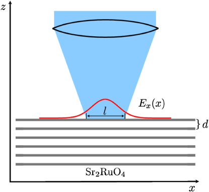
Figure 1: (color online). Schematic picture of the experimental setup in Ref. Xia06 . The incoming laser beam is incident normally to the conducting planes of the layered superconductor $\rm Sr_{2}RuO_{4}$. The beam is focused by the lens to a spot of the diameter $l$ at the surface of the sample. The solid (red) line shows the Gaussian profile of the polarized electric field $E_{x}$ in the beam (Ref. quarter-wave ). The interlayer distance in $\rm Sr_{2}RuO_{4}$ is $d$.

Equation (3) shows that the chiral current of a $p_{x}+ip_{y}$ superconductor directly couples to charge response and plasma collective modes. The Chern-Simons-type term (1) couples the longitudinal and transverse electromagnetic fields and leads to a number of interesting effects, that are not present in nonchiral superconductors. By taking a variation of Eq. (1) with respect to $A_{0}$, we find an anomalous charge response to the transverse electromagnetic field: $\delta\rho^{(a)}\propto B_{z}$, i.e., the charge is induced by the magnetic field $B_{z}$ along the $z$ direction Goryo00 ; Stone04 . In Sec. VII.2, we propose an experimental setup to directly verify this relationship. We also calculate how the relationship between $\delta\rho^{(a)}$ and $B_{z}$ is modified at high frequencies. By the continuity relation, the induced charge $\delta\rho^{(a)}$ produces an electric polarization current, which gives an additional contribution to the Hall effect of the same order as the magnetization current.

The paper is organized as follows. In Sec. II, we rigorously derive a general expression for the effective action of a Q2D $p_{x}+ip_{y}$ superconductor and obtain the gauge-invariant electromagnetic response. In Secs. III–V, we discuss the collective modes and the conventional and anomalous (chiral) electromagnetic responses. In Sec. VI, we obtain the symmetric and antisymmetric parts of the conductivity tensor of a chiral superconductor. In Sec. VII, we discuss the relationship of our results with the experimental studies of the chiral response of $\rm Sr_{2}RuO_{4}$. Finally, we summarize the results in Sec. VIII. Some technical details are relegated to the Appendixes. In particular, a simplified alternative derivation of the effective action is given in Appendix C.

II Effective action for a chiral quasi-two-dimensional $p_{x}+ip_{y}$ superconductor

II.1 Triplet $p_{x}+ip_{y}$ pairing

First, we briefly summarize basic information about the triplet $p$-wave pairing Leggett75 . The Cooper pairing between electrons is described by the pairing potential $\Delta_{\alpha\beta}(\bm{r},\bm{r}^{\prime})\propto\langle\psi_{\alpha}(\bm{r})\psi_{\beta}(\bm{r}^{\prime})\rangle$. Here, $\psi_{\alpha}(\bm{r})$ is the electron annihilation operator at the point $\bm{r}$ with the spin projection $\alpha=\uparrow,\downarrow$. For a uniform, translationally-invariant system, the pairing potential depends only on the relative distance $\bm{r}-\bm{r}^{\prime}$, so one can perform the Fourier transform and use the momentum representation $\Delta_{\alpha\beta}(\bm{p})\propto\langle\psi_{\alpha}(\bm{p})\psi_{\beta}(-\bm{p})\rangle$. The pairing tensor $\Delta_{\alpha\beta}(\bm{p})=\Delta(\bm{p})\,\bm{d}(\bm{p})\cdot{\bm{\sigma}}_{\alpha}^{\gamma}\,\eta_{\gamma\beta}$ can be written in terms of the antisymmetric metric tensor $\eta_{\gamma\beta}$ and the Pauli matrices ${\bm{\sigma}}_{\alpha}^{\gamma}$, where the unit vector $\bm{d}(\bm{p})$ characterizes the spin polarization of the triplet state. The prefactor $\Delta(\bm{p})$ is a momentum-dependent pairing amplitude.

For $\rm Sr_{2}RuO_{4}$, we consider the case where the vector $\bm{d}(\bm{p})=\hat{\bm{z}}$ has the uniform, momentum-independent orientation, which represents pairing between electrons with the opposite spins $\langle\psi_{\uparrow}(\bm{p})\psi_{\downarrow}(-\bm{p})\rangle$. (It can be transformed into pairing with parallel spins by changing the spin quantization axis.) For the orbital symmetry, we consider the chiral pairing potential $\Delta(\bm{p})=\Delta_{0}(p_{x}\pm ip_{y})/p_{F}$, where $p_{F}$ is the Fermi momentum, and $\Delta_{0}$ is the superconducting gap. This order parameter corresponds to a vortex in the momentum space, because the phase of $\Delta(\bm{p})$ changes by $\pm 2\pi$ when $\bm{p}$ goes around the Fermi surface. It is instructive to write the pairing potential in the form

$$\Delta(\bm{p})=\Delta_{x}p_{x}+i\Delta_{y}p_{y},$$ (6)

and set $\Delta_{x}=\pm\Delta_{y}=\Delta_{0}/p_{F}$ only at the end of the calculations. The sign of the product

$$s_{xy}\equiv{\rm sign}(\Delta_{x}\Delta_{y})$$ (7)

reflects the sign of the order-parameter chirality.

II.2 Theoretical model

Our goal is to derive an effective action for a chiral superconductor in a weak electromagnetic field. This approach is equivalent to a linear response calculation Schrieffer ; UFN ; Kulik ; Levin ; Das Sarma . We use the Greek indices, e.g., $\mu$ and $\nu$, to denote the space-time components of tensors in the Minkowski notation and the Roman indices, e.g., $k$ and $l$, for the space components. To simplify intermediate steps of calculations, we set the Planck constant $\hbar$, the Boltzmann constant $k_{B}$, and the speed of light $c$ to unity: $\hbar=k_{B}=c=1$. The constants $\hbar$ and $k_{B}$ can be easily restored in the final equations by dimensionality. The speed of light can be restored by noting that it appears only in the combination $\bm{A}/c$ with the vector potential $\bm{A}$. To simplify presentation, we first study a purely 2D case, which corresponds to just one metallic layer in the $(x,y)$ plane, and then generalize the calculation to the case of many coupled parallel metallic layers, as appropriate for $\rm Sr_{2}RuO_{4}$.

The Hamiltonian of interacting electrons, subject to an external electromagnetic field $A^{\mu}$, is given by

$$\hat{H} = \int d^{2}r\,\psi^{\dagger}_{\sigma}(\bm{r})\left(\frac{[\hat{\bm{p}}-e\bm{A}(\bm{r})]^{2}}{2m_{e}}-\mu\right)\psi_{\sigma}(\bm{r})$$

$$+ \int d^{2}r\,eA_{0}(\bm{r})\,\delta n(\bm{r})$$

$$- \int d^{2}r\,d^{2}r^{\prime}g(\bm{r}-\bm{r}^{\prime})\,\psi^{\dagger}_{\uparrow}(\bm{r})\psi^{\dagger}_{\downarrow}(\bm{r}^{\prime})\psi_{\downarrow}(\bm{r}^{\prime})\psi_{\uparrow}(\bm{r})$$

$$+ \frac{e^{2}}{2}\int d^{2}r\,d^{2}r^{\prime}\delta n(\bm{r})\,V(\bm{r}-\bm{r}^{\prime})\,\delta n(\bm{r}^{\prime}).$$

Here, $m_{e}$ and $\mu$ are the electron mass and the chemical potential, $g(\bm{r}-\bm{r}^{\prime})$ is an anisotropic interaction potential leading to a $p$-wave pairing, and $V(\bm{r}-\bm{r}^{\prime})=1/|\bm{r}-\bm{r}^{\prime}|$ is the Coulomb interaction potential. The density fluctuation operator $\delta n(\bm{r})$ reads

$$\delta n(\bm{r})=\psi^{\dagger}_{\sigma}(\bm{r})\psi_{\sigma}(\bm{r})-n_{0},$$ (9)

with $n_{0}$ being the 2D background charge density. The summation over repeated indices is assumed everywhere.

The starting point for our calculation is the partition function $Z$, which can be expressed as a path integral over the anticommuting fermionic fields $\psi$ and $\psi^{\dagger}$. We use the Hubbard-Stratonovich transformation to decouple the fermion interaction terms in Eq. (II.2) by introducing additional integrals over auxiliary bosonic fields $\Delta$ and $\varphi$ Negele ; Svidzinskii ; AES ; Otterlo ; Sharapov . The complex field $\Delta(\bm{r},\bm{r}^{\prime},\tau)$ is the superconducting pairing potential, and $\varphi(\bm{r},\tau)$ is the internal electric potential produced by electrons. As a result, the partition function, written in the imaginary time $\tau$, reads Euclidean

$$Z=\int\mathcal{D}\Delta^{*}\mathcal{D}\Delta\mathcal{D}\varphi\>e^{-S_{\rm bos}}\int\mathcal{D}\psi^{\dagger}\mathcal{D}\psi\>e^{-S_{\rm el}},$$ (10)

where the bosonic action is

$$S_{\rm bos}=ie\int d\tau d^{2}r\,[\varphi(\bm{r},\tau)+A_{0}(\bm{r},\tau)]\,n_{0}$$ (11)

$$+\int\!d\tau d^{2}r\,d^{2}r^{\prime}\left[\frac{|\Delta(\bm{r},\bm{r}^{\prime},\tau)|^{2}}{g(\bm{r}\!-\!\bm{r}^{\prime})}+\frac{\varphi(\bm{r},\tau)\varphi(\bm{r}^{\prime},\tau)}{2V(\bm{r}\!-\!\bm{r}^{\prime})}\right],$$

and the electronic action is

$$S_{\rm el}\!=\!\int\!d\tau d^{2}r\psi^{\dagger}_{\sigma}(\bm{r},\tau)\!\left(\frac{[\hat{\bm{p}}-e\bm{A}(\bm{r},\tau)]^{2}}{2m_{e}}-\mu\right)\!\psi_{\sigma}(\bm{r},\tau)$$

$$\!+\!\int\!d\tau d^{2}r\,\psi^{\dagger}_{\sigma}(\bm{r},\tau)\!\{\partial_{\tau}-ie[\varphi(\bm{r},\tau)\!+\!A_{0}(\bm{r},\tau)]\}\!\psi_{\sigma}(\bm{r},\tau)$$

$$\!-\!\int\!d\tau d^{2}rd^{2}r^{\prime}\left[\Delta(\bm{r},\bm{r}^{\prime},\tau)\psi^{\dagger}_{\uparrow}(\bm{r},\tau)\psi^{\dagger}_{\downarrow}(\bm{r}^{\prime},\tau)\!+\!\mathrm{H.c.}\right]\!\!.$$ (12)

The superconducting pairing potential in Eq. (12) can be written as a function of the relative coordinate $\bm{r}-\bm{r}^{\prime}$ and the center-of-mass coordinate $\bm{R}=(\bm{r}+\bm{r}^{\prime})/2$. For a uniform system, in the absence of electromagnetic field, the equilibrium saddle-point configuration of $\Delta_{0}$ in the total action (10) does not depend on $\bm{R}$ and $\tau$, and is given by Eq. (6) in the Fourier representation with respect to $\bm{r}-\bm{r}^{\prime}$. In the presence of an applied electromagnetic field, the saddle-point value of the complex superconducting pairing potential is shifted and can be written in the adiabatic Born-Oppenheimer approximation Sharapov ; Thouless as

$$\Delta(\bm{p},\bm{R},\tau)=\frac{p_{x}+ip_{y}}{p_{F}}[\Delta_{0}+\delta\Delta(\bm{R},\tau)]\,e^{i\Phi(\bm{R},\tau)}.$$ (13)

We assume here that the applied electromagnetic field is weak, and varies slowly in space and time, i.e., $\xi/\lambda\ll 1$ and $\omega\ll\omega_{\rm cutoff}<\varepsilon_{F}$. Here, $\lambda$ and $\omega$ are the wavelength and frequency of the electromagnetic field, $\xi=v_{F}/\Delta_{0}$ is the superconducting coherence length, $\omega_{\rm cutoff}$ is the cutoff frequency of the interaction responsible for superconducting pairing, and $\varepsilon_{F}$ is the Fermi energy. The field shifts the amplitude of the pairing potential by $\delta\Delta$ and gives a space-time dependence to the phase $\Phi$ of the order parameter. As in the $s$-wave superconductors, the amplitude variations $\delta\Delta$ are massive Kulik , and their contribution to the linear electromagnetic response is small in the parameter $(\Delta_{0}/\varepsilon_{F})^{2}\ll 1$ UFN . Therefore, we neglect the amplitude fluctuations in the rest of the paper and only consider the dynamics of the phase $\Phi$. The $p$-wave order parameter also has other modes, such as the clapping modes, due to its internal orbital structure Yip92 . However, these modes are also massive, and we do not consider them.

The phase $\Phi$ of the order parameter is essential for ensuring the gauge invariance of the theory. By performing a unitary transformation of the fermion operators $\psi_{\sigma}(\bm{r},\tau)\rightarrow e^{i\Phi(\bm{r},\tau)/2}\psi_{\sigma}(\bm{r},\tau)$, one can compensate the phase of the order parameter Sharapov . As a result, the electromagnetic field in Eq. (12) is replaced by the gauge-invariant combinations of electromagnetic potentials and the superconducting phase:

$$\tilde{A}_{0}=A_{0}-\partial_{\tau}\Phi/2e,\quad\tilde{\bm{A}}=\bm{A}-\bm{\nabla}\Phi/2e.$$ (14)

In this way, one ensures that the gauge invariance is fulfilled at every step of the calculation.

After the phase transformation, the superconducting pairing potential in Eq. (12) has the equilibrium value given by Eq. (6). The electron Lagrangian (12) can be written in the momentum-frequency representation as a $2\times 2$ Nambu matrix acting on the spinor $\bm{\psi}(p)=[\psi_{\uparrow}(\bm{p},\omega_{m}),\psi_{\downarrow}^{\dagger}(-\bm{p},\omega_{m})]$, where $\omega_{m}$ is the fermionic Matsubara frequency, and $p=(i\omega_{m},p_{x},p_{y})$,

$$S_{\rm el}=\sum_{p}\bm{\psi}^{\dagger}(p)\,G^{-1}(p)\,\bm{\psi}(p)$$ (15)

$$+\sum_{p,q}\bm{\psi}^{\dagger}(p+q)\Gamma_{1}(p,q)\bm{\psi}(p)+\sum_{p,q}\bm{\psi}^{\dagger}(p)\Gamma_{2}(p,q)\bm{\psi}(p).$$

Here, $\sum_{p}$ represents the integration over momenta as well as the summation over the Matsubara frequencies Gamma_2 . The terms $G^{-1}$, $\Gamma_{1}$, and $\Gamma_{2}$ in the electron action (15) contain the zeroth, first, and second powers of the electromagnetic fields $\tilde{A}^{\mu}$ and $\varphi$,

$$G^{-1}(p)\!\!\! = \!\!\!i\omega_{m}-\xi_{\bm{p}}\hat{\tau}_{3}-p_{x}\Delta_{x}\hat{\tau}_{1}+p_{y}\Delta_{y}\hat{\tau}_{2},$$ (16)

$$\Gamma_{1}(p,q)\!\!\! = \!\!\!-ie[\tilde{A}_{0}(q)+\varphi(q)]\hat{\tau}_{3}-e\bm{v}(\bm{p}+\bm{q}/2)\cdot\tilde{\bm{A}}(q),$$ (17)

$$\Gamma_{2}(p,q)\!\!\! = \!\!\!\frac{e^{2}}{2}\frac{\partial^{2}\xi_{\bm{p}}}{\partial p_{k}\partial p_{l}}\tilde{A}_{k}(q)\tilde{A}_{l}(-q)\hat{\tau}_{3}.$$ (18)

Here, the wave vector $\bm{q}$ of the electromagnetic field and its bosonic Matsubara frequency $\Omega_{n}$ are combined into $q=(i\Omega_{n},\bm{q})$. The electron dispersion and velocity are $\xi_{\bm{p}}=\bm{p}^{2}/2m_{e}-\mu$ and $\bm{v}(\bm{p})=\bm{p}/m_{e}$. Equations (16)–(18) are written in terms of the Pauli matrices $\hat{\tau}$ acting on the electron spinor $\bm{\psi}$.

II.3 Integrating out fermions

Substituting the action (15) into Eq. (10) and taking the functional integral over $\psi$, we obtain the electron contribution $S_{\rm eff}^{\rm el}$ to the effective action up to the second order in the electromagnetic fields $\tilde{A}^{\mu}$ and $\varphi$,

$$S_{\rm eff}^{\rm el}(\tilde{A}^{\mu},\varphi)=-\mathrm{Tr}\ln(G^{-1}+\Gamma_{1}+\Gamma_{2})=-\mathrm{Tr}\ln{G^{-1}}$$

$${}-\mathrm{Tr}\,{G\Gamma_{1}}-\mathrm{Tr}\,{G\Gamma_{2}}+\frac{1}{2}\mathrm{Tr}\,{G\Gamma_{1}G\Gamma_{1}}.$$ (19)

Here, $\mathrm{Tr}$ denotes both the matrix trace and the sum over the internal frequencies and momenta.

The term $\mathrm{Tr}\ln{G^{-1}}$ in Eq. (19) and the term proportional to $|\Delta|^{2}$ in Eq. (11) define the saddle point configuration (6) of the unperturbed system. The functional integral over the amplitude of $\Delta$ is taken by expansion in the vicinity of this saddle-point configuration. Combining the remaining terms in Eqs. (11) and (19), we obtain the effective phase-only action of the system

$$Z=\int\mathcal{D}\Phi\,\mathcal{D}\varphi\,\exp[-S_{\rm eff}(\tilde{A}^{\mu},\varphi)],$$ (20)

$$S_{\rm eff}(\tilde{A}^{\mu},\varphi)=\frac{1}{2}\sum_{q}\left[\frac{\varphi(q)\varphi(-q)}{V(\bm{q})}+\frac{e^{2}n_{0}}{m}\tilde{\bm{A}}(q)\cdot\tilde{\bm{A}}(-q)\right]$$

$$+\frac{1}{2}\mathrm{Tr}[G\Gamma_{1}G\Gamma_{1}].$$ (21)

Here, $V(\bm{q})$ is the Fourier transform of the Coulomb potential, which in 2D is equal to $V(\bm{q})=2\pi/|\bm{q}|$.

Now we need to evaluate the trace in Eq. (21). This amounts to calculation of one-loop Feynman diagrams using the fermionic Green’s function $G$ from Eq. (16),

$$G=-\frac{i\omega_{m}+\xi_{\bm{p}}\hat{\tau}_{3}+p_{x}\Delta_{x}\hat{\tau}_{1}-p_{y}\Delta_{y}\hat{\tau}_{2}}{\omega_{m}^{2}+\xi_{\bm{p}}^{2}+p_{x}^{2}\Delta_{x}^{2}+p_{y}^{2}\Delta_{y}^{2}},$$ (22)

and the vertex $\Gamma_{1}$ (17), which represents interaction with the electromagnetic field. The final expression for the effective action (21) can be written as

$$S_{\textrm{eff}}(\tilde{A}^{\mu},\varphi)=\frac{1}{2}\sum_{q}\frac{\varphi(q)\varphi(-q)}{V(\bm{q})}$$ (23)

$$+Q_{00}i[\tilde{A}_{0}(q)\!+\!\varphi(q)]i[\tilde{A}_{0}(\!-\!q)\!+\!\varphi(\!-\!q)]\!+\!Q_{kl}\tilde{A}_{k}(q)\tilde{A}_{l}(\!-\!q)$$

$$+iQ_{0k}[\tilde{A}_{0}(q)\!+\!\varphi(q)]\tilde{A}_{k}(\!-\!q)\!+\!iQ_{k0}\tilde{A}_{k}(q)[\tilde{A}_{0}(\!-\!q)\!+\!\varphi(\!-\!q)].$$

Here, $Q_{00}$, $Q_{kl}$, and $Q_{0k}(q)=Q_{k0}(-q)$ are the corresponding correlation (polarization) functions.

The density-density polarization function $Q_{00}=e^{2}{\rm Tr}[\tau_{3}G\tau_{3}G]$ is

$$\!Q_{00}\!=\!\int{\!\frac{d^{2}p}{(2\pi)^{2}}}\!\frac{2e^{2}}{\beta}\sum_{i\omega_{m}}\!\frac{i\omega_{m}(i\omega_{m}\!+\!i\Omega_{n})\!+\!\xi_{-}\xi_{+}\!-\!\Delta_{+}\Delta_{-}}{[(\omega_{m}\!+\!\Omega_{n})^{2}\!+\!E_{+}^{2}][\omega_{m}^{2}\!+\!E_{-}^{2}]}.$$ (24)

Here, $\beta=1/T$, $\xi_{\pm}=\xi_{\bm{p}\pm\bm{q}/2}$, $\Delta_{+}\Delta_{-}=\Delta_{x}^{+}\Delta_{x}^{-}\!+\!\Delta_{y}^{+}\Delta_{y}^{-}$, $E_{\pm}=\sqrt{\xi_{\pm}^{2}+(\Delta_{x}^{\pm})^{2}+(\Delta_{y}^{\pm})^{2}}$ with $\Delta_{x(y)}^{\pm}=(p_{x(y)}\pm q_{x(y)}/2)\Delta_{x(y)}$.

The current-current correlation function $Q_{kl}$ consists of the diamagnetic $Q^{(1)}_{kl}$ and paramagnetic $Q^{(2)}_{kl}=e^{2}{\rm Tr}[v_{k}Gv_{l}G]$ parts

$$\!\!Q_{kl}\! \!=\! \!Q^{(1)}_{kl}+Q^{(2)}_{kl},\quad\quad\quad\!\!Q^{(1)}_{kl}=\frac{e^{2}n_{0}}{m_{e}}\,\delta_{kl},$$ (25)

$$Q^{(2)}_{kl}\!\! \!\!=\!\! \!\!\int\!\!\frac{d^{2}p}{(2\pi)^{2}}\frac{2e^{2}v_{k}v_{l}}{\beta}\!\sum_{i\omega_{m}}\!\frac{i\omega_{m}(i\omega_{m}\!+\!i\Omega_{n})\!+\!\xi_{-}\xi_{+}\!+\!\Delta_{+}\Delta_{-}}{[(\omega_{m}\!+\!\Omega_{n})^{2}\!+\!E_{+}^{2}][\omega_{m}^{2}\!+\!E_{-}^{2}]},$$

with $\bm{v}=\partial\xi_{\bm{p}}/\partial\bm{p}=\bm{p}/m_{e}$ being the electron velocity.

The expressions (24), (25) and (LABEL:Qij1) for the density-density and current-current correlation functions are the same for chiral and nonchiral superconductors and contain nothing special. The only important difference between chiral and nonchiral superconductors appears in the structure of the current-density correlation function $Q_{k0}=e^{2}{\rm Tr}[v_{k}G\tau_{3}G]$. This difference plays the crucial role for the results of our paper. In a $p_{x}+ip_{y}$ superconductor, $Q_{k0}$ consists of the conventional, symmetric part $Q_{k0}^{(s)}$ and the anomalous, antisymmetric part $Q_{k0}^{(a)}$:

$$Q_{k0}\! \!\!=\!\! Q_{k0}^{(s)}+Q_{k0}^{(a)},$$ (27)

$$Q_{k0}^{(s)}\! \!\!=\!\! \!-\!\int{\frac{d^{2}p}{(2\pi)^{2}}}\!\frac{2e^{2}v_{k}}{\beta}\sum_{i\omega_{m}}\frac{(i\omega_{m}\!+\!i\Omega_{n})\xi_{-}\!+\!i\omega_{m}\xi_{+}}{[(\omega_{m}\!+\!\Omega_{n})^{2}\!+\!E_{+}^{2}][\omega_{m}^{2}\!+\!E_{-}^{2}]},$$

$$Q_{k0}^{(a)}\! \!\!=\!\! \!-\!\int{\frac{d^{2}p}{(2\pi)^{2}}}\!\frac{2e^{2}v_{k}}{\beta}\sum_{i\omega_{m}}\frac{[iq_{x}p_{y}\!-\!iq_{y}p_{x}]\Delta_{x}\Delta_{y}}{[(\omega_{m}\!+\!\Omega_{n})^{2}\!+\!E_{+}^{2}][\omega_{m}^{2}\!+\!E_{-}^{2}]}.$$

The two terms have the following symmetries

$$Q_{k0}^{(s)}(-q)=Q_{k0}^{(s)}(q),\quad Q_{k0}^{(a)}(-q)=-Q_{k0}^{(a)}(q),$$ (30)

where the operation $q\to-q$ means changing the signs of both frequency and momentum. Equation (30) follows from an observation that $Q_{k0}^{(s)}$ is proportional to a product of the frequency and momentum components of $q$, whereas $Q_{k0}^{(a)}$ is a linear function of the momentum components $q_{x}$ and $q_{y}$ only. One can also check using Eqs. (24), (25) and (LABEL:Qij1) that $Q_{00}(-q)=Q_{00}(q)$ and $Q_{kl}(-q)=Q_{kl}(q)$ are symmetric.

Equation (LABEL:Qj0a) shows that the anomalous charge-current correlation function $Q_{k0}^{(a)}$ explicitly depends on the chirality (7) of the order parameter, whereas the other correlation functions do not depend on it. We demonstrate in the rest of the paper that all of the non-trivial, chiral response of a $p_{x}+ip_{y}$ superconductor originates from the anomalous term (LABEL:Qj0a). The density-current correlator $Q_{k0}$ (27) is rarely discussed in textbooks and literature. Non-chiral superconductors have only the symmetric term $Q_{k0}^{(s)}$ (LABEL:Qj0s), which couples to the longitudinal degrees of freedom (see Sec. IV.1), such as plasmon collective modes, but does not affect the transverse response, such as the London-Meissner current. Therefore, for the calculation of the transverse response, it is sufficient to consider a gauge with $\bm{A}^{\perp}\neq 0$ and $A_{0}=0$. However, in chiral superconductors, the antisymmetric term $Q_{k0}^{(a)}$ couples to the transverse response (see Sec. V.1) and controls the TRS-breaking response of the system. In the technical language, when calculating the transverse response of the chiral superconductors, one has to include vertex corrections in order to obtain correct results. Without vertex corrections, calculations do not generate chiral terms in the electromagnetic response of a $p_{x}+ip_{y}$ superconductor Joynt91 ; Ting07 .

II.4 Integrating out the internal Coulomb potential

It is well-known that response functions of a charged superconductor, as opposed to a neutral superfluid such as ³He, are strongly modified by the Coulomb interaction. In our approach, integrating out the internal electric potential $\varphi$ is equivalent to taking into account the Coulomb interaction, because $\varphi$ mediates the electrostatic interaction between electrons. The effective action $S_{\rm eff}(\tilde{A}^{\mu})$, obtained after taking the functional integral over $\varphi$ in Eq. (20), is defined as follows:

$$Z=\int\mathcal{D}\Phi\,\mathcal{D}\varphi\,e^{-S_{\rm eff}(\tilde{A}^{\mu},\varphi)}=\int\mathcal{D}\Phi\,e^{-S_{\rm eff}(\tilde{A}^{\mu})}.$$ (31)

Substituting Eq. (23) into Eq. (31) and taking the Gaussian integral over $\varphi$, we find

$$S_{\rm eff}(\tilde{A}^{\mu})\! = \!\frac{1}{2}\sum_{q}\tilde{Q}_{00}i\tilde{A}_{0}(q)i\tilde{A}_{0}(-q)+\tilde{Q}_{kl}\tilde{A}_{k}(q)\tilde{A}_{l}(-q)$$ (32)

$$+ 2\tilde{Q}_{0k}i\tilde{A}_{0}(q)\tilde{A}_{k}(-q),$$

where the polarization functions are renormalized by the Coulomb interaction $V(\bm{q})$ as follows:

$$\tilde{Q}_{00}=\frac{Q_{00}(q)}{1-V(\bm{q})\,Q_{00}(q)},\quad\tilde{Q}_{k0}=\frac{Q_{k0}(q)}{1-V(\bm{q})\,Q_{00}(q)},$$

$$\tilde{Q}_{kl}=Q_{kl}+\frac{Q_{k0}V(\bm{q})\,Q_{0l}}{1-V(\bm{q})\,Q_{00}}.$$ (33)

The renormalized polarization functions (33) can be equivalently obtained through the resummation of the most diverging diagrams due to the Coulomb interaction in the random phase approximation (RPA) as shown in Fig. 2.

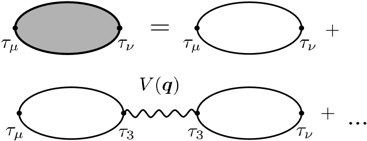
Figure 2: Renormalization of the polarization functions (33) due to the Coulomb interaction $V(\bm{q})$ in the RPA. The wavy line denotes $V(\bm{q})$, which couples only to the charge vertices represented by the Pauli matrices $\tau_{3}$.

II.5 Integrating out the superconducting phase

We integrate out the superconducting phase $\Phi$ to obtain the gauge-invariant effective action $S_{\rm eff}(A^{\mu})$ that depends only on the electromagnetic field $A^{\mu}$ as follows:

$$Z=e^{-S_{\rm eff}(A^{\mu})}=\int\mathcal{D}\Phi\,e^{-S_{\rm eff}(\tilde{A}^{\mu})},$$ (34)

where the field $\tilde{A}^{\mu}$ is defined by Eq. (14) and contains $\Phi$. Substituting Eq. (32) into Eq. (34) and taking the Gaussian integral over $\Phi$, we finally obtain the effective action Kosztin

$$S_{\rm eff}(A^{\mu}) = \frac{1}{2}\sum_{q}K_{\mu\nu}(q)A^{\mu}(q)A^{\nu}(-q),$$ (35)

$$K_{\mu\nu} = \tilde{Q}_{\mu\nu}-\frac{\tilde{Q}_{\mu\rho}q^{\rho}q^{\sigma}\tilde{Q}_{\sigma\nu}}{\tilde{Q}_{\alpha\beta}q^{\alpha}q^{\beta}}.$$ (36)

Notice that the kernel (36) satisfies the identity

$$q^{\mu}K_{\mu\nu}=K_{\mu\nu}q^{\nu}=0,$$ (37)

which ensures that the effective action (35) is gauge-invariant. Indeed, in the momentum representation, the gauge transformation is $A^{\mu}\to A^{\mu}-iq^{\mu}\phi$, where $\phi$ is an arbitrary scalar function. Substituting this expression into Eq. (35) and taking into account the identities (37), we see that the additional terms $q^{\mu}\phi$ drop out and, thus, the effective action is gauge-invariant.

II.6 Generalization to the quasi-two-dimensional case

The derivation presented in the previous sections can be easily generalized to a Q2D system consisting of parallel superconducting layers separated by the distance $d$ in the $\hat{\bm{z}}$ direction. The layers are coupled via the interlayer electron tunneling amplitude $t_{c}$. In the tight-binding approximation, the electron dispersion and velocity are

$$\xi_{\bm{p}}=\frac{p_{x}^{2}+p_{y}^{2}}{2m_{e}}-t_{c}\cos(p_{z}d)-\mu,\quad\bm{v}(\bm{p})=\frac{\partial\xi_{\bm{p}}}{\partial\bm{p}},$$ (38)

where $(p_{x},p_{y})$ and $p_{z}$ are the in-plane and out-of-plane momenta, respectively. We assume that the interlayer tunneling amplitude is much smaller than the in-plane Fermi energy: $t_{c}\ll\varepsilon_{F}$. Then, the Fermi surface is a slightly warped cylinder extended in the $p_{z}$ direction. Equation (38) should be substituted into Eqs. (24)–(LABEL:Qj0a), where the integrals should be taken over a three-dimensional (3D) momentum $\bm{p}$, with $p_{z}$ limited to the interval $[-\pi/d,\pi/d]$.

The diamagnetic term $Q^{(1)}_{kj}$ in Eq. (25) should be replaced by the expression following from Eq. (18) Sharapov

$$Q^{(1)}_{kl}\!=\!e^{2}\!\int\!\frac{d^{3}p}{(2\pi)^{3}}\left[1-\frac{\xi_{\bm{p}}}{E_{\bm{p}}}\tanh\left(\frac{E_{\bm{p}}}{2T}\right)\right]\frac{\partial^{2}\xi_{\bm{p}}}{\partial p_{k}\,\partial p_{l}},$$ (39)

where $E_{\bm{p}}=\sqrt{\xi_{\bm{p}}^{2}+|\Delta(\bm{p})|^{2}}$. The integrals (39) can easily be evaluated and give the following expression for the diamagnetic tensor of a Q2D superconductor:

$$Q_{kl}^{(1)}=\frac{e^{2}n_{0}}{m_{e}d}\,\tensor{n}_{kl},\quad\tensor{n}=\left(\begin{array}[]{ccc}1&0&0\\ 0&1&0\\ 0&0&\displaystyle\frac{t_{c}^{2}m_{e}d^{2}}{2\varepsilon_{F}}\end{array}\right).$$ (40)

Here, $n_{0}=p_{F}^{2}/2\pi$ is the 2D electron density, and $p_{F}$, $v_{F}$, and $\varepsilon_{F}=p_{F}^{2}/2m_{e}$ are the in-plane Fermi momentum, velocity, and energy. The dimensionless tensor $\tensor{n}$ represents the anisotropy of the superfluid density.

In a layered Q2D system, the renormalized polarization functions $\tilde{Q}_{\mu\nu}$ are given by Eq. (33) with the appropriate form of the Coulomb interaction Das Sarma :

$$V(\bm{q})=\frac{2\pi d}{|\bm{q}_{\|}|}\frac{\sinh(|\bm{q}_{\|}|d)}{\cosh(|\bm{q}_{\|}|d)-\cos(q_{z}d)},$$ (41)

where $\bm{q}_{\|}=(q_{x},q_{y})$. Equation (41) reduces to the 3D expression for the Coulomb potential $V_{\rm 3D}(\bm{q})$ at small momenta $|\bm{q}|d\ll 1$ and to the 2D Fourier transform of the Coulomb potential $V_{\rm 2D}(\bm{q}_{\|})$ in the limit $|\bm{q}_{\|}|d\gg 1$ as follows:

$$V_{\rm 3D}(\bm{q})=\frac{4\pi}{\bm{q}^{2}},\quad V_{\rm 2D}(\bm{q}_{\|})=\frac{2\pi d}{|\bm{q}_{\|}|}.$$ (42)

In the long-wavelength limit ($|\bm{q}|d\ll 1$) considered in the rest of our paper, the appropriate form of the Coulomb potential is $V_{\rm 3D}(\bm{q})$.

II.7 Linear response

By taking a variation of Eq. (35) with respect to $A^{\mu}$, we obtain the gauge-invariant electromagnetic response of the system,

$$j_{\mu}(q)=K_{\mu\nu}(q)A^{\nu}(q).$$ (43)

Notice that the identities (37) ensure that the current (43) satisfies the continuity equation $q^{\mu}j_{\mu}=0$.

To obtain physical results, we perform an analytical continuation from the Matsubara frequency to the real frequency $i\Omega_{n}\rightarrow\omega+i\delta$ Euclidean . After the continuation, the vector $q$ becomes $q^{\mu}=(\omega,\bm{q})$, and Eq. (43) gives a causal response to the external electromagnetic field $A^{\mu}=(A_{0},\bm{A})$ at a finite temperature $T$. The kernel $K_{\mu\nu}(q)$ is defined via Eqs. (33) and (36) in terms of the one-loop response functions (24)-(LABEL:Qj0a). Their analytical continuations to the real frequency after summation over the fermionic Matsubara frequencies are given in Appendix A.

III Collective modes

Under certain conditions, an infinitesimal external electromagnetic field can induce a large current or density response of the system, which indicates the existence of internal collective excitations in the superconductor. These resonances occur when the denominator in Eq. (36) goes to zero. Using Eq. (33), the denominator can be written as $\tilde{Q}_{\mu\nu}q^{\mu}q^{\nu}=\tilde{R}(\omega,\bm{q})/[1-V(\bm{q})\,Q_{00}]$, where the function $\tilde{R}(\omega,\bm{q})$ is defined as

$$\tilde{R}(\omega,\bm{q}) = Q_{kl}q_{k}q_{l}+2\omega Q_{0l}^{(s)}q_{l}+\omega^{2}Q_{00}$$ (44)

$$+ V(\bm{q})\,(Q_{0k}^{(s)}Q_{l0}^{(s)}-Q_{00}Q_{kl})\,q_{k}q_{l}.$$

Notice that only the conventional tensor $Q_{l0}^{(s)}$ appears in Eq. (44). The anomalous tensor $Q_{k0}^{(a)}$ does not appear because it is transverse, as will be discussed in Sec. V.1. The dispersion relation for the collective modes is determined by the equation $\tilde{R}(\omega,\bm{q})=0$.

In the limit of small $|\bm{q}|$, we can simplify Eq. (44) by keeping only the nonvanishing terms $Q_{00}$ and $Q_{kl}$ in the first and second lines of Eq. (44), whereas the terms $Q_{k0}^{(s)}$ and $Q_{kl}^{(2)}$ vanish in this limit. Using Eq. (40) for $Q_{kl}^{(1)}$, we find the dispersion relation for the collective modes at $T=0$,

$$\omega^{2}=V(\bm{q})\frac{e^{2}n_{0}}{m_{e}d}\left(\bm{q}_{\|}^{2}+\frac{t_{c}^{2}m_{e}d^{2}}{\varepsilon_{F}}\,q_{z}^{2}\right).$$ (45)

In the case $|\bm{q}|d\ll 1$, it is appropriate to use the 3D limit $V_{\rm 3D}(\bm{q})$ from Eq. (42) for the Coulomb interaction in Eq. (45) and, thus, we find the following spectrum of collective modes Hirschfeld1993 ; Levin ; Das Sarma :

$$\omega^{2}=\frac{\omega_{ab}^{2}\bm{q}_{\|}^{2}+\omega_{c}^{2}q_{z}^{2}}{\bm{q}_{\|}^{2}+q_{z}^{2}}=\omega_{ab}^{2}\,\frac{\bm{q}\cdot\tensor{n}\cdot\bm{q}}{\bm{q}^{2}}.$$ (46)

Here, the tensor $\tensor{n}$ is defined in Eq. (40), and $\omega_{ab}$ and $\omega_{c}$ are the in-plane and out-of-plane plasma frequencies,

$$\omega_{ab}^{2}=4\pi\frac{e^{2}n_{0}}{m_{e}d},\qquad\omega_{c}^{2}=2\pi\frac{e^{2}t_{c}^{2}dn_{0}}{\varepsilon_{F}}.$$ (47)

As shown in Appendix B, the collective mode (46) corresponds to coupled plasma oscillations of the internal electric potential and the superconducting phase $\Phi$. The plasma mode frequency (46) depends on the ratio of the in-plane $\bm{q}_{\|}$ and out-of-plane $q_{z}$ momenta HwangDasSarma98 . Plasma oscillations are gapped in all directions, but are strongly anisotropic due to the smallness of the interlayer tunneling amplitude $t_{c}$. The experimental values of the plasma frequencies in $\rm Sr_{2}RuO_{4}$ are $\omega_{c}=0.32$ eV and $\omega_{ab}=4.5$ eV Tokura96 ; Tokura01 .

If one formally sets $t_{c}=0$ and uses the 2D expression for the Coulomb potential from Eq. (42), then Eq. (45) gives the plasmon mode dispersion for a single 2D layer

$$\omega_{\bm{q}}=\sqrt{\frac{2\pi n_{0}e^{2}}{m_{e}}|\bm{q}_{\|}|}.$$ (48)

However, this limit does not correspond to $\rm Sr_{2}RuO_{4}$.

At higher temperatures $T\rightarrow T_{c}$, there may be long-wavelength oscillations with the acoustic spectrum. These oscillations are neutral and consist of supercurrent oscillations compensated by oscillations of the normal current, as discovered by Carlson and Goldman Goldman . However, at $T\ll T_{c}$ only the plasma mode survives, because the normal density is exponentially suppressed.

IV CONVENTIONAL NONCHIRAL ELECTROMAGNETIC RESPONSE

IV.1 Transverse and longitudinal tensors

First, we describe general properties of the tensors $Q_{kl}$ and $Q_{k0}^{(s)}$. It is convenient to separate the symmetric tensor $Q_{kl}$ into the longitudinal $Q_{kl}^{\|}$ and transverse $Q_{kl}^{\perp}$ parts defined by the following relations

$$Q_{kl}=Q_{kl}^{\|}+Q_{kl}^{\perp},$$ (49)

$$q_{k}Q_{kl}^{\|}=q_{k}Q_{kl},\quad Q_{kl}^{\|}q_{l}=Q_{kl}q_{l},$$ (50)

$$q_{k}Q_{kl}^{\perp}=Q_{kl}^{\perp}q_{l}=0.$$ (51)

Equations (50)–(51) have the following general solution

$$Q_{kl}^{\|}=\frac{Q_{kr}q_{r}q_{s}Q_{sl}}{q_{u}Q_{uv}q_{v}},\quad Q_{kl}^{\perp}=Q_{kl}-Q_{kl}^{\|}.$$ (52)

In the dynamic limit, $\omega\neq 0$ and $\bm{q}\to 0$, which is relevant for optical measurements, the paramagnetic term $Q_{kl}^{(2)}$, defined in Eq. (121), vanishes, and $Q_{kl}$ is given by the diamagnetic term (40). Then, the transverse and longitudinal parts of the tensor $Q_{kl}$ are

$$Q^{\perp}_{kl} = \frac{\omega_{ab}^{2}}{4\pi}\left(\tensor{n}-\frac{(\tensor{n}\cdot\bm{q})(\bm{q}\cdot\tensor{n})}{\bm{q}\cdot\tensor{n}\cdot\bm{q}}\right)_{kl},$$ (53)

$$Q^{\|}_{kl} = \frac{\omega_{ab}^{2}}{4\pi}\left(\frac{(\tensor{n}\cdot\bm{q})(\bm{q}\cdot\tensor{n})}{\bm{q}\cdot\tensor{n}\cdot\bm{q}}\right)_{kl}.$$ (54)

The conventional current-density correlation function $Q_{k0}^{(s)}$, given by Eq. (122), is an odd function of $\bm{q}$ and $\omega$. The term $Q_{k0}^{(s)}$ satisfies the following identity for small $\bm{q}$:

$$Q_{0k}^{(s)}=Q_{kl}^{\|}q_{l}\,\frac{q_{u}Q_{u0}}{q_{r}Q_{rs}^{\|}q_{s}}.$$ (55)

To prove Eq. (55), we observe that the tensor structure of $Q_{kl}=\int v_{k}v_{l}\ldots$ and $Q_{k0}^{(s)}=\int v_{k}\ldots$ in Eqs. (39), (121), and (122) is determined by the electron velocities $\bm{v}=\partial\xi_{\bm{p}}/\partial\bm{p}$. Since the term $Q_{k0}^{(s)}$ vanishes at $\bm{q}=0$, the leading-order expansion of the integrand is proportional to $v_{k}v_{l}q_{l}$, i.e., $Q_{k0}^{(s)}=\int v_{k}v_{l}q_{l}\ldots$. Thus, in the long-wavelength limit, we have $Q_{k0}^{(s)}\propto Q_{kl}q_{l}$, which leads to Eq. (55). Equation (122) gives the following explicit expression for $Q^{(s)}_{k0}$ for small $\bm{q}$ and finite $\omega$ at $T=0$:

$$Q^{(s)}_{k0}=-\frac{\omega_{ab}^{2}}{4\pi}\frac{\omega(\tensor{n}\cdot\bm{q})_{k}}{\Delta_{0}^{2}}\int_{1}^{\infty}\frac{dx}{x^{2}\sqrt{x^{2}-1}}$$ (56)

$$\times\frac{1}{2x+(\omega+i\delta)/\Delta_{0}}\,\frac{1}{2x-(\omega+i\delta)/\Delta_{0}}.$$

We see that $Q^{(s)}_{k0}$ is proportional to the tensor $\tensor{n}$ multiplied by $\bm{q}$, which is consistent with Eq. (55).

IV.2 Conventional nonchiral electromagnetic response

We now show that if we omit the anomalous chiral term (LABEL:Qj0a) in Eqs. (33) and (36), we recover the conventional response of a superconductor to the electromagnetic field. Using Eqs. (33) and (49) and the identity (55), we obtain the following expression for the space-time components of the conventional response kernel $K_{\mu\nu}^{(c)}$ (36):

$$K_{kl}^{(c)}=Q_{kl}^{\perp}-\omega^{2}\tilde{\kappa}_{kl},\quad K_{00}^{(c)}=-q_{k}\tilde{\kappa}_{kl}q_{l},$$ (57)

$$K_{l0}^{(c)}=K_{0l}^{(c)}=\omega q_{k}\tilde{\kappa}_{kl}.$$

In the long-wavelength limit assumed here, the transverse tensor $Q_{kl}^{\perp}$ is given by Eq. (53), and the longitudinal tensor $\tilde{\kappa}_{kl}$ is defined as follows:

$$\tilde{\kappa}_{kl}=\frac{Q_{k0}^{(s)}Q_{0l}^{(s)}-Q_{kl}^{\|}Q_{00}}{\tilde{R}},$$ (58)

with the function $\tilde{R}(\omega,\bm{q})$ given by Eq. (44). By using Eq. (57), the charge and current responses (43) can be written in the following form:

$$\delta\rho = -i\bm{q}\cdot\bm{P},$$ (59)

$$\bm{j} = -\,\tensor{Q}^{\perp}\cdot\bm{A}-i\omega\bm{P},$$ (60)

$$\bm{P} = \tensor{\tilde{\kappa}}\cdot\bm{E}^{\rm ext}.$$ (61)

Here $\delta\rho$ and $\bm{j}$ are the induced charge and current densities, and $\bm{P}$ is the polarization vector. In Eq. (60) we use the shorthand notation $[\,\tensor{Q}^{\perp}\,]_{kl}\equiv Q^{\perp}_{kl}$ [see Eq. (53)].

Equation (61) expresses $\bm{P}$ in terms of the external electric field $\bm{E}^{\rm ext}=-i\bm{q}A_{0}+i\omega\bm{A}$ (We remind the reader that the electromagnetic potential $A^{\mu}$ in our calculations represents the external field.) $\bm{E}^{\rm ext}$ is connected to the total electric field $\bm{E}^{\rm tot}$, which includes the field created by other electrons in the system, by the standard relation

$$\bm{E}^{\rm ext}=\bm{E}^{\rm tot}+4\pi\bm{P}=\tensor{\varepsilon}\cdot\bm{E}^{\rm tot},$$ (62)

where $\tensor{\varepsilon}$ is the tensor of dielectric permeability. If we expressed the polarization vector $\bm{P}$ in Eq. (61) as a linear function of the total electric field $\bm{E}^{\rm tot}$, then the corresponding proportionality tensor would be the dielectric susceptibility tensor $\kappa_{kl}$ Landau . However, because Eq. (61) expresses $\bm{P}$ as a function of the external field $\bm{E}^{\rm ext}$, the corresponding tensor $\tilde{\kappa}_{kl}$ is the RPA-renormalized dielectric susceptibility tensor, which includes the effect of charge screening via the RPA diagrams shown in Fig. 2.

The tensor $\tilde{\kappa}_{kl}$ in Eq. (58) can be simplified in the limit of small $\bm{q}$. In this case, the terms involving $Q_{k0}^{(s)}$ in the numerator and denominator of Eq. (58) can be neglected relative to the other terms because $Q_{k0}^{(s)}$ vanishes at $\bm{q}\to 0$. Using this approximation and Eq. (44), we rewrite Eq. (58) in terms of the longitudinal tensor $Q_{kl}^{\|}$ (54) as follows:

$$\tensor{\tilde{\kappa}} = -\frac{\alpha(\omega,\bm{q})}{\omega_{ab}^{2}}\,\tensor{Q}^{\|},$$ (63)

$$\alpha(\omega,\bm{q}) = \frac{\omega_{ab}^{2}Q_{00}}{\bm{q}\cdot\tensor{Q}\cdot\bm{q}+\omega^{2}Q_{00}-V(\bm{q})\,Q_{00}\,\bm{q}\cdot\tensor{Q}\cdot\bm{q}}.$$ (64)

Here, the dimensionless function $\alpha(\omega,\bm{q})$ describes screening of charge in the static case and plasma oscillations in the dynamic case.

Indeed, in the static limit $\omega=0$, the function $Q_{00}$, given by Eq. (120), is proportional to the density of states

$$Q_{00}(\omega=0)=-2e^{2}N_{0}/d,\quad N_{0}=m_{e}/2\pi,$$ (65)

where $N_{0}$ is the 2D density of states per spin. Then Eq. (64) for $\omega=0$ reads

$$\alpha^{(s)}(\omega=0,\bm{q})=-\frac{1}{(\bm{q}\cdot\tensor{n}\cdot\bm{q})}\frac{q_{{TF}}^{2}}{1+q_{\rm TF}^{2}/\bm{q}^{2}},$$ (66)

where $q_{\rm TF}$ is the inverse Thomas-Fermi screening length

$$q_{\rm TF}^{2}=8\pi e^{2}N_{0}/d.$$ (67)

Thus, Eq. (66) describes the electrostatic screening of charge in an anisotropic conductor.

In the dynamic case $\omega\gg v_{F}|\bm{q}|$, we neglect the first term in the denominator of Eq. (64) and obtain

$$\alpha^{(d)}(\omega,\bm{q})=\frac{\omega_{ab}^{2}}{\omega^{2}-[\omega_{ab}^{2}(\bm{q}\cdot\tensor{n}\cdot\bm{q})/\bm{q}^{2}]}.$$ (68)

Equation (68) exhibits a resonance, signifying a divergence of the charge response, when the frequency $\omega$ approaches to the plasma frequency defined in Eq. (46).

Equations (58)–(61) coincide with the results of Ref. UFN [Cf. with Eqs. (28) and (29) of Ref. UFN , which were obtained using an exact solution for vertex functions]. Note that the transverse part of the current response in Eq. (60) is not affected by the collective modes Schrieffer , whereas the charge response Eq. (59) is strongly affected by the collective dynamics of the superconducting phase and the Coulomb interaction. Equations (59) and (60) satisfy the continuity equation $\omega\,\delta\rho=\bm{q}\cdot\bm{j}$ and are invariant with respect to gauge transformations of the electromagnetic field. In anisotropic superconductors, it is not practical to separate $\bm{A}$ and $\bm{E}^{\rm ext}$ into longitudinal and transverse components, because such separation does not diagonalize the response equations (59) and (60), unlike in the isotropic case.

V Anomalous chiral electromagnetic response

V.1 Anomalous current-density correlation function

The chiral anomalous current-density correlation function $Q_{k0}^{(a)}$ is given by Eq. (123). By separating the factors $q_{x}$ and $q_{y}$, it can be written as

$$Q^{(a)}_{k0}=i\Theta\left(\begin{array}[]{c}q_{y}\\ -q_{x}\\ 0\\ \end{array}\right)_{k}=i\Theta\,\eta_{kl}q_{l}=i\Theta\,\check{q}_{k},$$ (69)

where $\eta_{xy}=-\eta_{yx}=1$ is the 2D antisymmetric tensor, and $\check{q}_{k}$ is the $k$th component of the vector

$$\check{\bm{q}}=\hat{\bm{z}}\times\bm{q}.$$ (70)

The anomalous term $Q_{k0}^{(a)}$ (69) is transverse: $q_{k}Q_{k0}^{(a)}=0$, unlike the conventional term $Q_{k0}^{(s)}$ in Eqs. (55) and (56).

In the limit $\bm{q}\to 0$, we obtain the following expression for the function $\Theta(\omega)$ from Eq. (123):

$$\Theta(\omega) = \frac{e^{2}\Delta_{x}\Delta_{y}}{m_{e}}\int{\frac{d^{3}p}{(2\pi)^{3}}}\frac{p_{x}^{2}+p_{y}^{2}}{4E^{2}}\,[1-2f(E)]$$ (71)

$$\times \left(\frac{1}{2E+\omega+i\delta}+\frac{1}{2E-\omega-i\delta}\right),$$

which was found before in Ref. Yakovenko07 . Changing the variable of integration to $x=E/\Delta_{0}$ and taking into account that the integral converges near the Fermi surface, we express Eq. (71) in the following form at $T=0$:

$$\Theta(\omega) = s_{xy}\,\frac{e^{2}}{2hd}\,I(\omega),\quad\quad I(0)=1,$$ (72)

$$I(\omega) = \int\limits_{1}^{\infty}\frac{dx}{\sqrt{x^{2}-1}}\,\frac{1}{x^{2}-[(\omega+i\delta)/2\Delta_{0}]^{2}}.$$ (73)

We restored the dimensional constants in Eq. (72). The sign of $\Theta$ is determined by the chirality $s_{xy}$ of the superconducting condensate. The function $I(\omega)$ has the following asymptotic behavior I(omega) :

$$I(\omega)\approx\left\{\begin{array}[]{ll}\displaystyle-4\left(\frac{\Delta_{0}}{\omega}\right)^{2}\ln\left(\frac{\omega}{\Delta_{0}}\right)+2\pi i\left(\frac{\Delta_{0}}{\omega}\right)^{2},&\omega\gg\Delta_{0}\\ \displaystyle 1,&\omega\ll\Delta_{0}.\end{array}\right.$$ (74)

The crossover between the two limiting cases occurs at $\omega\sim 2\Delta_{0}$, where the photon energy is equal to the binding energy between two electrons in a Cooper pair. The real and imaginary parts of $I(\omega)$ are shown in Fig. 3. The imaginary part is zero for $\omega<2\Delta_{0}$ and diverges as $1/\sqrt{\omega-2\Delta_{0}}$ when $\omega$ approaches $2\Delta_{0}$ from above. The real part is approximately constant at low frequencies and diverges as $1/\sqrt{2\Delta_{0}-\omega}$ when $\omega$ approaches $2\Delta_{0}$ from below. Both real and imaginary parts go to zero at $\omega\to\infty$.

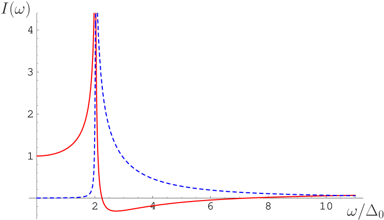
Figure 3: (color online). Frequency dependence of the function $I(\omega)$ given by Eq. (73). This function determines the frequency dependence of the ac Hall conductivity (113) of a chiral $p_{x}+ip_{y}$ superconductor in the dynamic limit. The solid (red) and dashed (blue) lines show the real and imaginary parts of $I(\omega)$.

V.2 Anomalous chiral electromagnetic response

Now we collect the terms that contain the chiral anomalous correlator $Q_{k0}^{(a)}$ in the kernel $K_{\mu\nu}$ (36). First, we notice that $Q_{k0}^{(a)}$ does not appear in the denominator $\tilde{Q}_{\alpha\beta}q^{\alpha}q^{\beta}$ of Eq. (36), because the denominator is longitudinal, whereas $Q_{k0}^{(a)}$ is transverse. Then, Eq. (36) contains only the linear and quadratic terms in $Q_{k0}^{(a)}$. The quadratic in $Q_{k0}^{(a)}$ term may be called the “double-anomalous.” Although this term has an anomalous origin, it is not chiral, i.e., it does not change sign under the time-reversal operation or when the chirality $s_{xy}$ of the order parameter changes sign. This term turns out to be small in the relativistic parameter $(v_{F}/c)^{2}$ and is not particularly important. The discussion of this term is deferred to Appendix C.

In the rest of the paper, we concentrate on the linear in $Q_{k0}^{(a)}$ terms in the response. Using Eq. (36), one obtains the following expression for the space-time components of the anomalous chiral kernel $K_{\mu\nu}^{(a)}$:

$$K_{kl}^{(a)}=i\omega\Theta\frac{\check{q}_{k}W_{l}-W_{k}\check{q}_{l}}{\tilde{R}},\quad K_{00}^{(a)}=0,$$ (75)

$$K_{l0}^{(a)}(q)=-K_{0l}^{(a)}(q)=i\Theta\check{q}_{l}\frac{q_{k}W_{k}}{\tilde{R}}.$$

Here, $\tilde{R}$, $\Theta$, and $\check{q}_{k}$ are given by Eqs. (44), (69), and (70), and the vector $\bm{W}$ is defined as

$$W_{k}=Q_{kl}^{\|}q_{l}+Q_{k0}^{(s)}\omega.$$ (76)

By using Eq. (75), the anomalous charge and current responses (43) can be written in the following form:

$$\delta\tilde{\rho}^{(a)} = -i\bm{q}\cdot\bm{P}^{(a)},$$ (77)

$$\bm{j}^{(a)} = i\bm{q}\times\bm{M}^{(a)}-i\omega\bm{P}^{(a)},$$ (78)

where $\bm{M}^{(a)}$ and $\bm{P}^{(a)}$ can be identified as the chiral magnetization and polarization White-Geballe ; Landau and are given by

$$\bm{P}^{(a)} = -i\Theta\bm{W}\frac{[\bm{q}\times\bm{E}^{\rm ext}]\cdot\hat{\bm{z}}}{\omega\tilde{R}}=-i\Theta\frac{\bm{W}}{\tilde{R}}B^{\rm ext}_{z},$$ (79)

$$\bm{M}^{(a)} = i\hat{\bm{z}}\,\Theta\frac{(\bm{W}\cdot\bm{E}^{\rm ext})}{\tilde{R}}.$$ (80)

Here, $B^{\rm ext}_{z}$ is the $z$ component of the external magnetic field $\bm{B}^{\rm ext}$, which is related to $\bm{E}^{\rm ext}$ via Maxwell’s equation $\bm{q}\times\bm{E}^{\rm ext}=\omega\bm{B}^{\rm ext}$. Both $\bm{M}^{(a)}$ and $\bm{P}^{(a)}$ in Eqs. (79) and (80) are proportional to the chiral response function $\Theta$ (72) and, thus, change sign when the chirality $s_{xy}$ of the order parameter changes sign. The peculiar feature of chiral superconductors is that the electric polarization $\bm{P}^{(a)}$ (79) is induced by the magnetic field $B_{z}$, whereas the magnetization $\bm{M}^{(a)}$ (80) couples to the longitudinal electric field. The first and second terms in Eq. (78) give the transverse and longitudinal components of the anomalous current, respectively.

In the limit of small $|\bm{q}|$, by using Eqs. (54) and (56) and the condition $I(0)=1$, the vector $\bm{W}$ in Eq. (76) can be written as

$$W_{k}=q_{l}Q_{lk}^{\|}+\omega Q^{(s)}_{0k}=I(\omega)\,\frac{\omega_{ab}^{2}}{4\pi}(\tensor{n}\cdot\bm{q})_{k},$$ (81)

where $I(\omega)$ is given by Eq. (73). In the same limit, only the terms proportional to $Q_{00}$ survive in the function $\tilde{R}$ given by Eq. (44). Using Eq. (120) at $\bm{q}\to 0$, we find that

$$Q_{00}(\omega)=-\frac{2e^{2}N_{0}}{d}\,I(\omega),$$ (82)

where $I(\omega)$ again is given by Eq. (73). Then, with the help of Eqs. (81), (82), and (44), we find that

$$\frac{\bm{W}}{\tilde{R}}=-\frac{\alpha(\omega,\bm{q})\,d}{4e^{2}m_{e}}\,(\tensor{n}\cdot\bm{q}),$$ (83)

where the function $\alpha(\omega,\bm{q})$ is given by Eq. (64). Using Eq. (83), the expressions (79) and (80) for $\bm{P}^{(a)}$ and $\bm{M}^{(a)}$ can be written as

$$\bm{P}^{(a)} = i\Theta\,\frac{\alpha(\omega,\bm{q})\,d}{4e^{2}m_{e}}\,\frac{[\bm{q}\times\bm{E}^{\rm ext}]\cdot\hat{\bm{z}}}{\omega}\,(\tensor{n}\cdot\bm{q})$$

$$= i\Theta\,\frac{\alpha(\omega,\bm{q})\,d}{4e^{2}m_{e}}\,B^{\rm ext}_{z}\,(\tensor{n}\cdot\bm{q}),$$

$$\bm{M}^{(a)} = -i\hat{\bm{z}}\,\Theta\,\frac{\alpha(\omega,\bm{q})\,d}{4e^{2}m_{e}}\,(\bm{q}\cdot\tensor{n}\cdot\bm{E}^{\rm ext}).$$ (85)

The static and dynamic limits of Eqs. (V.2) and (85) can be obtained by taking appropriate limits (66) and (68) for the function $\alpha(\omega,\bm{q})$.

V.3 Discussion of the anomalous magnetization current

By comparing Eq. (85) for the anomalous magnetization with the expression for the induced conventional charge density from Eqs. (59), (61), (63), and (54), one can notice that $\bm{M}^{(a)}$ can be expressed in terms of $\delta\rho$

$$\bm{M}^{(a)}=-s_{xy}\,\hat{\bm{z}}\,\frac{I(\omega)}{4m_{e}}\,\delta\rho.$$ (86)

Then, the first term in Eq. (78), the magnetization current, can be written in real space as

$$\bm{j}_{M}^{(a)}(\omega,\bm{r})=s_{xy}\,\frac{I(\omega)}{4m_{e}}\,[\hat{\bm{z}}\times\bm{\nabla}\delta\rho(\omega,\bm{r})].$$ (87)

At $\omega=0$, Eq. (87) reduces to expression (3) for the Mermin-Muzikar current Mermin80 , which was discussed in Sec. I. However, at high frequencies, the anomalous magnetization current (87) is suppressed by the function $I(\omega)\propto(\Delta_{0}/\omega)^{2}$ [see Eq. (74)]. The general reason for this suppression is that physical manifestations of the low-energy Cooper pairing with the angular momentum $L_{z}=\hbar$ should fade away at high frequencies $\omega\gg\Delta_{0}$. Indeed, the electron states at high energies are essentially the same as in a normal metal, so the properties of the system should approach those of a normal metal at high frequencies. The suppression of the anomalous magnetization current at high frequencies is one of the reasons why the Kerr angle is so small Mineev07 . Equation (87) gives an important generalization of the Mermin-Muzikar current to arbitrary frequencies.

In order to calculate the magnetization current correctly, it is very important to take into account the term $Q^{(s)}_{0k}$ in Eq. (81). This term vanishes at $\omega=0$ and can be neglected at low frequencies, as was done in Refs. Goryo98 ; Goryo99 ; Goryo00 ; Golub03 ; Stone04 . However, at high frequencies, Eq. (56) shows that $Q^{(s)}_{0k}\propto-q_{k}/\omega$, and, in the leading order of approximation, the second term of the sum in Eq. (81) cancels the first term. The remaining difference gives the small factor $I(\omega)\propto(\Delta_{0}/\omega)^{2}$. The term $Q_{00}$ is also proportional to $I(\omega)$ in Eq. (82), so the factors $I(\omega)$ in $\bm{W}$ and $\tilde{R}$ cancel out in Eq. (83), but $\Theta(\omega)$ produces the factors $I(\omega)$ in Eqs. (85), (86), and (87). If $Q^{(s)}_{0k}$ were neglected in Eq. (81), then $\bm{W}$ would have a constant value at high frequencies, and one would incorrectly conclude that Eq. (3) is valid for arbitrarily high frequencies. The asymptotic cancellation of the two terms in the sum in Eq. (81) can also be shown using the Ward identities UFN .

V.4 Discussion of the anomalous polarization current

The second term $\bm{j}_{P}^{(a)}$ in Eq. (78) is determined by the chiral polarization $\bm{P}^{(a)}$. Although $\bm{j}_{P}^{(a)}$ is formally proportional to $\omega$, it contributes equally to the total current even at low frequencies. Indeed, Eqs. (79) and (V.2) show that the chiral polarization diverges at low frequencies as $1/\omega$. This divergence exactly cancels $\omega$ in Eq. (78), which results in a finite contribution from the chiral polarization to the current even at low frequencies. Both magnetization and polarization currents equally contribute to the Hall conductivity tensor, which is discussed below in Eqs. (106) and (112). The anomalous polarization current $\bm{j}_{P}^{(a)}$ was often omitted in the previous papers in the low frequency limit.

Equations (77), (79), and (V.2) show that the magnetic field $B_{z}$ induces an anomalous electric charge, as mentioned in Sec. I. The polarization current $\bm{j}_{P}^{(a)}$ in Eq. (78) is necessary to satisfy the continuity equation for the anomalous charge in Eq. (77).

V.5 Anomalous chiral effective action

Substituting the components (75) of the anomalous tensor $K_{\mu\nu}^{(a)}$ into Eq. (35), we obtain the chiral part of the gauge-invariant effective action for the electromagnetic field as

$$\tilde{S}_{\rm eff}^{(a)}=-i\sum_{q}\Theta(q)\,\frac{\bm{W}(q)\cdot\bm{E}^{\rm ext}(q)}{\tilde{R}(q)}\,B^{\rm ext}_{z}(-q)$$

$$\approx i\frac{s_{xy}}{8hm_{e}}\sum_{q}\alpha(\omega,\bm{q})\,I(\omega)\,[\bm{q}\cdot\tensor{n}\cdot\bm{E}^{\rm ext}(q)]\,B^{\rm ext}_{z}(-q).$$ (88)

Given that Eq. (75) is written for the real frequency $\omega$, we write Eq. (88) for the real frequency as well. The anomalous charge and current responses, given by Eqs. (77)–(80), can be obtained by taking the appropriate variations of Eq. (88). The causality of the response function should be properly addressed, as discussed in Ref. Negele .

Unlike the conventional action for the electromagnetic field, the anomalous action (88) involves a product of the electric and magnetic fields. Thus, the anomalous action (114) breaks the TRS, because $\bm{E}\to\bm{E}$ and $\bm{B}\to-\bm{B}$ upon the time-reversal operation. Equation (114) is manifestly gauge-invariant and is a replacement for the Chern-Simons-type term (1) after integration out of the superconducting phase $\Phi$. The calculation of this action is one of the central results of our paper. A simplified alternative derivation of the effective action is also given in Appendix C.

Anomalous effective actions of the forms similar to Eq. (88) were obtained for chiral superfluids in Refs. Goryo98 ; Goryo99 ; Golub03 . Coupling between the electric and magnetic fields was discussed in Ref. Ishikawa98 . However, because these calculations were performed in the low-frequency limit, they did not obtain the factor $I(\omega)$, which suppresses the chiral effects at high frequencies, as discussed in Sec. V.3. The factor $\tilde{R}$ in the denominator of Eq. (88) represents the collective modes of the system. References Goryo98 ; Goryo99 ; Golub03 did not take into account the Coulomb interaction, which is appropriate for electrically neutral superfluids, such as ³He. Thus, the collective modes in the denominator of the effective actions in these papers were the acoustic modes of the superconducting phase, which can be obtained by setting $V(\bm{q})=0$ in Eq. (44). However, in the case of a charged superconductor, the collective modes are the gapped plasmons represented by the function $\tilde{R}$ in Eq. (88) (see also Ref. Golub03 ). One should keep in mind that, because we have integrated out the internal Coulomb potential, the electromagnetic field in Eq. (88) is the external one. Depending on the physical context, it may also be useful to study the chiral response with respect to the total electromagnetic field, which includes both external and internal fields. This problem is discussed in Sec. VI.

VI Conductivity tensor of a chiral superconductor

VI.1 Response to the external versus total electric field

In order to calculate the polar Kerr angle (see Appendix D) and other observable experimental quantities, one needs to know the conductivity tensor $\tensor{\sigma}$ of a chiral superconductor, which is defined by the standard relation

$$\bm{j}=\tensor{\sigma}\cdot\bm{E}^{\rm tot}.$$ (89)

Here, $\bm{E}^{\rm tot}$ is the total electric field inside the superconductor. In principle, the tensor $\tensor{\sigma}$ can be extracted from Eqs. (60) and (78) for the conventional and chiral currents. However, the polarization and magnetization vectors in these equations are expressed by Eqs. (61), (79), and (80) in terms of the external electric field $\bm{E}^{\rm ext}$. These equations give the linear response relation in the form

$$\bm{j}=\tensor{\tilde{\sigma}}\cdot\bm{E}^{\rm ext}$$ (90)

with a different tensor $\tensor{\tilde{\sigma}}$ Mahan , which includes the renormalization due to the RPA diagrams shown in Fig. 2.

The linear response relation in the form (90) is physically transparent, because it gives a direct response of the system to the external perturbation. However, in general, the response of the system to the external field depends on the geometry of the sample and the experimental apparatus. Only in the idealized case of an infinite uniform system can the problem be solved by the Fourier transform. To deal with this problem, the standard approach in the electrodynamics of continuous media Landau is to use the constituency relation (89), which expresses the response of the media to the total electromagnetic field in terms of the conductivity tensor characterizing the material. The constituency relations are substituted into Maxwell’s equations as the source terms, and then Maxwell’s equations are solved with the boundary conditions appropriate for the experimental setup. This is how, for example, one can take into account the Meissner screening, which was not included in the RPA-renormalized linear response given by Eq. (90).

In order to obtain the proper constituency relations, we need to transform the results of the paper to the form (89). This can easily be done by noticing that, in Eq. (12), the internal (induced) electric potential $\varphi$ appears next to the external potential $A_{0}$. Thus, the combined electric potential corresponds to the total electric field $\bm{E}^{\rm tot}$ inside the superconductor. Then, Eq. (23) gives the effective action for the total electromagnetic field. By taking a variational derivative with respect to the total electromagnetic field, one arrives at Eq. (89). Formally, this means that we do not integrate out the internal field $\varphi$ and do not perform the RPA renormalization of the response kernels $Q_{\alpha\beta}$ in Eq. (33). Thus, the transition between Eqs. (90) and (89) can be accomplished by setting $V(\bm{q})=0$ and replacing $\bm{E}^{\rm ext}$ with $\bm{E}^{\rm tot}$ in the electromagnetic response. The Coulomb potential $V(\bm{q})$ appears explicitly only in the function $\tilde{R}(\omega,\bm{q})$ defined in Eq. (44). Therefore, one should replace this function with the bare one acoustic ,

$$R(\omega,\bm{q}) = Q_{kl}q_{k}q_{l}+2\omega Q_{0k}^{(s)}q_{k}+\omega^{2}Q_{00}.$$ (91)

Using this prescription and Eqs. (60) and (78), one can easily obtain the conductivity tensor

$$\tensor{\sigma}=\tensor{\sigma}^{(c)}+\tensor{\sigma}^{(a)},$$ (92)

which consists of the conventional (nonchiral) $\tensor{\sigma}^{(c)}$ and the anomalous (chiral) $\tensor{\sigma}^{(a)}$ contributions, as discussed below.

VI.2 Conventional nonchiral conductivity tensor

Following the prescription of Sec. VI.1 and using Eqs. (58), (60) and (61), we obtain the conventional part of the conductivity tensor as follows:

$$\tensor{\sigma}^{(c)} = \tensor{\sigma}^{(1)}+\tensor{\sigma}^{(2)},$$ (93)

$$\tensor{\sigma}^{(1)}_{kl} = -\frac{1}{i\omega}Q_{kl}^{\perp},$$ (94)

$$\tensor{\sigma}^{(2)}_{kl} = -i\omega\frac{(Q_{k0}^{(s)}Q_{0l}^{(s)}-Q_{kl}^{\|}Q_{00})}{R},$$ (95)

where the function $R(\omega,\bm{q})$ is given by Eq. (91).

In the dynamic limit $\omega\neq 0$ and $\bm{q}\to 0$, the terms $Q_{k0}^{(s)}$ in the numerator of Eq. (95) and the terms proportional to $\bm{q}$ in Eq. (91) vanish. As a result, the expression for the conductivity tensor is simplified

$$\tensor{\sigma}^{(1)}_{kl}=-\frac{1}{i\omega}Q_{kl}^{\perp},\qquad\tensor{\sigma}^{(2)}_{kl}=-\frac{1}{i\omega}Q_{kl}^{\|}.$$ (96)

From Eq. (96), we find the total conductivity tensor in the long wavelength limit as follows:

$$\tensor{\sigma}^{(c)}_{kl}=-\frac{Q_{kl}^{(1)}}{i\omega}=-\frac{1}{4\pi i\omega}\left(\begin{array}[]{ccc}\omega_{ab}^{2}&0&0\\ 0&\omega_{ab}^{2}&0\\ 0&0&\omega_{c}^{2}\end{array}\right),$$ (100)

where we used Eq. (40) for $Q_{kl}^{(1)}$.

Combining Eq. (100) with the standard formula for the dielectric permeability tensor $\tensor{\epsilon}$,

$$\tensor{\epsilon}=\tensor{1}+\frac{4\pi i}{\omega}\tensor{\sigma},$$ (101)

we obtain

$$\tensor{\epsilon}(\omega)=\left(\begin{array}[]{ccc}1-\frac{\omega_{ab}^{2}}{\omega^{2}}&0&0\\ 0&1-\frac{\omega_{ab}^{2}}{\omega^{2}}&0\\ 0&0&1-\frac{\omega_{c}^{2}}{\omega^{2}}\end{array}\right).$$ (105)

Equations (100) and (105) represent the standard Drude response of an anisotropic conductor.

VI.3 Anomalous chiral conductivity tensor

The anomalous chiral response of the system to the total electric field is obtained from Eqs. (77)–(80) by replacing $\tilde{R}\to R$, where the function $R(\omega,\bm{q})$ is given by Eq. (91). From Eqs. (78)–(80) for the current response, we obtain the anomalous chiral conductivity tensor

$$\tensor{\sigma}^{(a)}_{kl}=\Theta\,\frac{\check{q}_{k}W_{l}-W_{k}\check{q}_{l}}{R},$$ (106)

where $\check{\bm{q}}$ and $W_{k}$ are given by Eqs. (70) and (76). Notice that the anomalous conductivity tensor is antisymmetric $\sigma^{(a)}_{kl}(q)=-\sigma^{(a)}_{lk}(q)$ and represents the intrinsic Hall conductivity of a chiral superconductor.

Using Eq. (81), we can rewrite the anomalous conductivity tensor (106) as

$$\tensor{\sigma}^{(a)}=\frac{\omega_{ab}^{2}\Theta(\omega)I(\omega)}{4\pi R(\omega,\bm{q})}\left[\check{\bm{q}}\,(\bm{q}\cdot\tensor{n})-(\tensor{n}\cdot\bm{q})\,\check{\bm{q}}\right]$$ (107)

$$=\frac{\omega_{ab}^{2}\Theta I}{4\pi R}\left(\begin{array}[]{ccc}0&-(q_{x}^{2}+q_{y}^{2})&-\zeta q_{y}q_{z}\\ q_{x}^{2}+q_{y}^{2}&0&\zeta q_{x}q_{z}\\ \zeta q_{y}q_{z}&-\zeta q_{x}q_{z}&0\end{array}\right),$$ (111)

where $\zeta=\omega_{c}^{2}/\omega_{ab}^{2}$ is a small parameter representing anisotropy of the band dispersion in a Q2D metal. The tensor components $\sigma^{(a)}_{zx}$ and $\sigma^{(a)}_{zy}$ in Eq. (111) are small, unless $q_{z}^{2}\gg\zeta^{2}(q_{x}^{2}+q_{y}^{2})$.

Now we concentrate on the $\sigma^{(a)}_{xy}$ component of the anomalous conductivity tensor (111)

$$\sigma^{(a)}_{xy}=-\Theta(\omega)\,\frac{\omega_{ab}^{2}\,I(\omega)}{4\pi R(\omega,\bm{q})}\,q_{\|}^{2},\quad q_{\|}^{2}=q_{x}^{2}+q_{y}^{2}.$$ (112)

It was argued in Refs. Yakovenko07 ; Mineev07 that the Hall conductivity of a chiral superconductor can be obtained by omitting the last term in the brackets of Eq. (4), which gives $\sigma^{(a)}_{xy}=\Theta(\omega)$. However, Eq. (112) shows that the systematic integration out of the superconducting phase $\Phi$ produces a different expression for $\sigma^{(a)}_{xy}$, which differs from $\Theta(\omega)$ by the additional factor proportional to $q_{\|}^{2}$. This factor involves the in-plane wave vector of the electromagnetic field and, in the appropriate limit, makes $\sigma^{(a)}_{xy}$ vanish when $q_{\|}^{2}\to 0$. This fact reflects the cancellation of the Hall effect Kallin for a uniform (in the plane) system discussed in Sec. I. Equation (112) is the central result of our paper and will be used in Sec. VII to estimate the observable Kerr effect. At low frequencies $\omega\ll\Delta_{0}$, where $I\approx 1$, Eq. (112) agrees with the corresponding results of Refs. Golub03 ; Goryo98 . However, at higher frequencies $\omega\geq\Delta_{0}$, the function $I(\omega)$ exhibits the nontrivial frequency dependence shown in Fig. 3. This behavior originates from the tendency to cancel between the current-current $Q_{kl}$ and current-density $Q^{(s)}_{k0}$ polarization functions in Eq. (81). Thus, it is essential to take $Q^{(s)}_{k0}$ into account at high frequencies (see discussion in Sec. V.3).

Let us discuss Eq. (112) in different limits. First, we consider the static limit $\omega=0$, set $q_{z}=0$, and then take $\bm{q}_{\|}\to 0$. Using Eqs. (72) and (91), we see that $q_{\|}^{2}$ cancels out, and we find that $\sigma^{(a)}_{xy}=e^{2}/2hd$, which is reminiscent of the quantum Hall effect Volovik88 ; Mineev07 ; Yakovenko07 . However, this formally calculated value does not correspond to an observable dc Hall effect. The static limit describes the system in thermodynamic equilibrium, where an applied electric field causes an inhomogeneous equilibrium redistribution of the electron density. As a result of the nonzero Cooper-pair angular momentum, the inhomogeneous electron density produces the equilibrium magnetization current Eq. (87). However, the total magnetization current flowing through any cross section of the sample, including the bulk and the edges, is zero, because the current is solenoidal. Therefore, the total current measured by an ammeter is zero. Thus, the formally calculated $\sigma^{(a)}_{xy}$ does not represent a measurable Hall effect dcHall .

The experimentally relevant limit is the dynamic limit with $\omega\neq 0$ and small $\bm{q}$. Taking this limit in Eq. (112) and using Eqs. (91) and (82), we find

$$\sigma^{(a)}_{xy}=\Theta(\omega)\,\frac{v_{F}^{2}q_{\|}^{2}}{2\omega^{2}},$$ (113)

where $v_{F}$ is the in-plane Fermi velocity. Equation (113) gives the ac Hall conductivity, where the frequency dependence of $\Theta(\omega)$ is given by Eqs. (72) and (73). Equation (113) differs from the expression $\sigma^{(a)}_{xy}=\Theta(\omega)$ obtained in the previous papers Yakovenko07 ; Mineev07 by the small factor $v_{F}^{2}q_{\|}^{2}/2\omega^{2}$.

VI.4 Anomalous effective action and charge response

Equation (88) gives the anomalous effective action as a function of the external electromagnetic field. Transformation of this action to the total field is straightforward by replacing $\tilde{R}\to R$ acoustic ,

$$S_{\rm eff}^{(a)}=-i\sum_{q}\Theta(q)\,\frac{\bm{W}(q)\cdot\bm{E}^{\rm tot}(q)}{R(q)}\,B^{\rm tot}_{z}(-q)$$

$$\approx i\frac{v_{F}^{2}}{2}\sum_{q}\Theta(\omega)\,\frac{[\bm{q}\cdot\tensor{n}\cdot\bm{E}^{\rm tot}(q)]\,B^{\rm tot}_{z}(-q)}{\omega^{2}-v_{F}^{2}(\bm{q}\cdot\tensor{n}\cdot\bm{q})/2}.$$ (114)

The difference between Eqs. (88) and (114) is that the former involves the gapped plasmon modes represented by $\tilde{R}$ (44) in the denominator, whereas the latter involves the acoustic modes of the superconducting phase represented by $R$ (91). This difference occurs because the two effective actions are written using the screened and unscreened electric fields, whereas the magnetic field is not screened by the internal Coulomb potential. For small $\bm{q}$ and high $\omega$, this difference amounts to using $R\approx Q_{00}\omega^{2}$ vs $\tilde{R}\approx Q_{00}[\omega^{2}-\omega_{ab}^{2}(\bm{q}\cdot\tensor{n}\cdot\bm{q})/\bm{q}^{2}]$, where the last term represents the momentum-dependent plasma frequency. The effective action is also discussed in Appendix C.

By taking a variational derivative of the action (114) with respect to the total field $A_{0}^{\rm tot}$, we find the anomalous electric charge induced by the magnetic field charge ,

$$\delta\rho^{(a)}=-\frac{\omega_{ab}^{2}}{4\pi}\,\frac{\Theta I}{R}\,(\bm{q}\cdot\tensor{n}\cdot\bm{q})\,B_{z}^{\rm tot}.$$ (115)

In the static limit, Eq. (115) reads

$$\delta\rho^{(a)}=-s_{xy}\,\frac{e^{2}}{2hdc}\,B_{z}^{\rm tot}.$$ (116)

Equation (116) was derived earlier in Refs. Goryo00 ; Stone04 and was mentioned in Sec. I. It is reminiscent of the S̆treda formula for the quantum Hall effect Streda . However, at high frequencies, Eq. (115) shows that the induced electric charge is significantly reduced relative to the static limit (116)

$$\delta\rho^{(a)}=s_{xy}\,\frac{e^{2}}{2hdc}\,I(\omega)\,\frac{v_{F}^{2}(\bm{q}\cdot\tensor{n}\cdot\bm{q})}{2\omega^{2}}\,B_{z}^{\rm tot}.$$ (117)

It is instructive to calculate how much electric charge would be induced by the static magnetic field of one superconducting vortex. If we take an integral $\int dx\,dy$ of Eq. (116), the left-hand side gives us the total induced electric charge, and the right-hand side gives the total magnetic flux. Taking the latter to be one superconducting flux quantum $\phi_{0}=hc/2e$, we find that the total induced electric charge in a vortex $\delta Q_{\rm vortex}$ is

$$\delta Q_{\rm vortex}=-s_{xy}\,\frac{e}{4}$$ (118)

per layer, i.e., the superconducting vortex has a fractional electric charge. Equation (118) was obtained by Goryo Goryo00 , who also pointed out that a vortex has a fractional angular momentum. However, the anomalous induced charge (118) would be screened by the conventional screening mechanism charge , and its experimental measurement may be challenging. It should be emphasized that the charge density (116) is not concentrated in the vortex core at the coherence length, but extends to the London penetration length, where the magnetic field is present. A possible experiment for detection of the anomalous induced electric charge is discussed in Sec. VII.2.

VII Experimental implications

VII.1 Polar Kerr effect experiment

In this section, we apply the derived theoretical results to the interpretation of the Kerr effect measurements Xia06 . We use the relationship between the Hall conductivity $\sigma_{xy}$ and the Kerr angle $\theta_{K}$ as presented in Appendix D.

First, we briefly discuss the estimates of the polar Kerr angle in the previous literature Yakovenko07 ; Mineev07 , where the formula $\sigma^{(a)}_{xy}=\Theta(\omega)$ was used without the additional factor appearing in Eq. (113). To estimate the Kerr angle, Ref. Yakovenko07 implicitly assumed that the refraction coefficient $n$ is real by using the value $n(n^{2}-1)=3$ quoted in Ref. Xia06 and expressed $\theta_{K}$ in terms of $\sigma_{xy}^{\prime\prime}$ via Eq. (140). The theoretical estimate given in Ref. Yakovenko07 is $\theta_{K}\approx 230$ nrad, which is of the same order of magnitude as the experimental value of 65 nrad Xia06 . In Ref. Mineev07 , a more detailed estimate was presented, using Eq. (142) for the refraction coefficient $n$ and discussing different limits $\omega>\omega_{p}$ and $\omega<\omega_{p}$. However, the factor $\epsilon_{\infty}$ was overlooked in Ref. Mineev07 as well as the presence of the real part $\sigma_{xy}^{\prime}(\omega)$, which gives the primary contribution to $\theta_{K}$ for $\omega<\omega_{p}$ ( see Appendix D). Overall, the numerical estimate of $\theta_{K}$ given in Ref. Mineev07 is of the same order of magnitude as in Ref. Yakovenko07 .

However, as discussed in Sec. I, Refs. Yakovenko07 and Mineev07 did not take into account the self-consistent dynamics of the superconducting phase $\Phi$ and, thus, missed the additional factor in Eq. (113), which makes the Hall conductivity dependent on the wave vector $q_{\|}$. In this case, strictly speaking, one cannot use the equations for $\theta_{K}$ presented in Appendix D, because they were derived for the normally-incident infinite plane wave with $q_{\|}=0$. However, as shown in Fig. 1, the experiment Xia06 was performed with a tightly focused Gaussian laser beam, which has nonzero Fourier components with $q_{\|}\neq 0$. Solving the boundary value problem for a reflection of a finite-size Gaussian beam from a chiral superconductor and determining the Kerr angle for polarization rotation is a complicated problem, that is beyond the scope of this paper. Nevertheless, to make a crude estimate of the Kerr angle, we can use the equations from Appendix D and the Hall conductivity given by Eq. (113) with the replacement $q_{\|}\to 1/l$, where $l$ is the typical transverse size of the Gaussian beam ( see Fig. 1). Taking into account that $\omega=c|\bm{q}|$, where the wave vector $|\bm{q}|=2\pi/\lambda$ is related to the wavelength of light $\lambda$, we can roughly estimate the Hall conductivity in Eq. (113) as

$$\sigma_{xy}\sim\Theta(\omega)\left(\frac{v_{F}}{c}\right)^{2}\left(\frac{\lambda}{l}\right)^{2}.$$ (119)

Using the values $v_{F}=5.5\times 10^{4}$ m/s for the $\gamma$ sheet of the Fermi surface Mackenzie03 , $c=3\times 10^{8}$ m/s, $\lambda=1.55$ $\mu$m, $l\sim 25$ $\mu$m Xia06 , and $\Delta_{0}=0.8$ meV  Sengupta02 in Eqs. (145) and (119), we estimate the Kerr angle to be $\theta_{K}\sim 10^{-14}$ rad. This estimate for $\theta_{K}$ is about 6 orders of magnitude smaller than the experimental value of $65$ nrad. The strong suppression of the Kerr angle relative to the previous estimate originates primarily from the small relativistic factor $(v_{F}/c)^{2}$ in Eq. (119).

In the rest of this section, we speculate about possible ways of resolving the discrepancy between the theory and experiment. As discussed in Sec. I, the general arguments of Ref. ReadGreen show that the intrinsic Hall conductivity should vanish for a spatially homogeneous uniform system. One way to break the translational symmetry is by taking into account the finite size $l$ of the laser beam. Then, inevitably, the Kerr angle acquires a dependence on $l$ as shown in Eq. (5), which is a very robust theoretical result. This proportionality relation should be checked experimentally.

Although the dependence on $l$ introduces a small factor, there may be mechanisms for enhancement of the response of the system, which may compensate for this additional smallness. One possibility is a resonance with the plasma modes. Equation (87) shows that the magnetization current is produced by the gradients of electron density. Therefore, the problem of the chiral current calculation reduces to how much electron charge is induced on the surface of a crystal by the inhomogeneous laser beam. The continuity of the electric field lines in a Gaussian beam in vacuum requires that the electric field components $E_{z}$ must be present at the periphery of the beam, even though the electric field is nominally polarized along $E_{x}$ at the center of the beam. This is well known for the fiber-optics modes, which have similarities with the Gaussian mode in vacuum Meschede . When the Gaussian beam hits the sample (see Fig. 1), the $E_{z}$ components induce electric charges of opposite signs on the two sides of the beam in the $x$ direction, which induce the electric current $j_{y}\propto q_{x}E_{z}$ according to Eq. (87). The induced electric current $j_{y}$ generates a magnetic field $B_{x}$ and a reflected electromagnetic wave with the $E_{y}$ polarization. Taking into account that $E_{z}\propto(q_{\|}/|\bm{q}|)E_{x}$, we obtain the same result as in Eq. (113). However, because the external electric field $E_{z}$ directly couples to the induced electron charge, the response of the system would be enhanced by the factor $\alpha^{(d)}(\omega,\bm{q})$ in Eq. (68) when the frequency of light $\omega$ is in resonance with one of the plasma modes. As discussed in Appendix D, the experimental frequency $\omega$ is in between the upper and lower plasma frequencies $\omega_{ab}>\omega>\omega_{c}$ and, thus, $\omega$ can be in resonance with one of the plasma modes (46) for some vector $\bm{q}$. Besides, because of the boundary at $z=0$ between the sample and vacuum, it may be necessary to solve for the plasma modes more accurately by taking into account the surface plasmons as well.

Another reason for the discrepancy in the magnitude of the Kerr effect may be the idealization of our theoretical model. Indeed, we considered the electromagnetic response of a clean superconductor in the presence of particle-hole symmetry. Within this model, Eqs. (120)–(123) for the response kernels are written assuming momentum conservation for the electrons. A more realistic model has to take into account the effect of impurities, in which case the momentum conservation does not hold. Indeed, one of the reasons for smallness of $\theta_{K}$ within our model can be traced back to the cancellation of the two terms in Eq. (81) at high frequencies. As a result, the right-hand side of Eq. (81) is small in the parameter $(\Delta_{0}/\hbar\omega)^{2}\sim 10^{-6}$. If we take into account impurities, the complete cancellation in Eq. (81) might not hold, and the estimate for $\theta_{K}$ would be significantly larger. Indeed, in the derivation of this equation, we assumed that the paramagnetic kernel $Q^{(2)}_{kl}$ given in Eq. (121) vanishes in the dynamic limit ($\omega\neq 0$ and $\bm{q}\to 0$). However, it is well known from the classic paper by Mattis and Bardeen Mattis-Bardeen that $Q^{(2)}_{kl}$ does not vanish when impurity scattering is taken into account. This term plays a significant role by taking away some spectral weight from the London-Meissner supercurrent, which makes the superconducting gap visible in optical measurements. For $\rm Sr_{2}RuO_{4}$, this fact was experimentally confirmed in Ref. Ormeno , which found that the superfluid density at $T=0$ is reduced by $22\%$. Therefore, the cancellation in Eq. (81) in the presence of disorder should be investigated in a future theoretical work.

VII.2 Proposed experiments

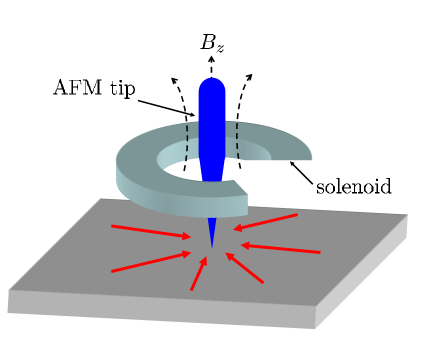
Figure 4: (color online). Schematic setup of a proposed experiment to measure the electric charge induced by a magnetic field perpendicular to the layers in $\rm Sr_{2}RuO_{4}$, as given by Eq. (116). A current in the solenoid or the coil produces a magnetic field $B_{z}$ inducing an electric charge at the center, which is carried by the radial currents shown by the arrows. The induced charge is detected by the AFM tip.

As discussed in Sec. VI.4, the magnetic field component $B_{z}$ applied perpendicular to the conducting planes of $\rm Sr_{2}RuO_{4}$ is expected to induce an electric charge. The effect is stronger in the static limit than in the dynamic limit. In this section, we propose a conceptual experiment to verify this effect. The schematic experimental setup is shown in Fig. 4. A miniature solenoid or a coil carrying electric current creates a magnetic field with the $B_{z}$ component. The current and the magnetic field are modulated at a low frequency (a few kilohertz), so that the quasistatic formula (116) is applicable newexp , but the lock-in measurements are enabled. The slowly alternating magnetic field $B_{z}$ induces an alternating electric charge near the center of the coil, which is produced by the radial alternating currents, shown by the arrows in Fig. 4. The induced electric charge is detected by a sensitive atomic force microscope (AFM) tip, shown as the pointed vertical object in Fig. 4. The AFM tip should be made from a nonmagnetic but highly electrical polarizable material to reduce the response to magnetic fields and enhance the response to the electric charge. To increase sensitivity, measurements should be performed at the lock-in frequency of the current in the coil. The difference of the signals above and below the superconducting transition temperature should be taken in order to subtract the background effects. A noticeable increase of the signal below $T_{c}$ would signify the observation of the effect. Then, the measurements can be performed at different locations on the sample. If a superconducting domain of the opposite chirality is found, the effect would change sign, i.e., the sign of the induced electric charge would change vs the sign of the applied magnetic field. It may be possible to map out the chiral domain boundaries in this way, assuming that the domains are sufficiently static and do not fluctuate in time too fast.

VIII Conclusions

In this paper, we studied the electromagnetic response of a Q2D chiral $p_{x}+ip_{y}$ superconductor, such as $\rm Sr_{2}RuO_{4}$. By integrating out the superconducting phase $\Phi$, we obtained the gauge-invariant effective action of the system in an electromagnetic field. Besides the well-known conventional terms, this action also contains an anomalous chiral term, which breaks the time-reversal symmetry. Instead of the Chern-Simons-type term (1), discussed in the earlier literature Volovik88 ; Furusaki01 ; Yakovenko07 , the gauge-invariant anomalous effective action (114) contains a product of the electric and magnetic fields. This is rather unusual situation, and the modified Chern-Simons-type term (114) leads to a number of interesting effects.

By taking variations of the anomalous effective action with respect to the electromagnetic potentials $A^{\mu}$, we obtained the anomalous charge and current responses of the system. We found that the transverse chiral response couples to the collective plasma modes, while the anomalous charge response manifests itself as the electric charge induced by the magnetic field $B_{z}$ perpendicular to the conducting layers of $\rm Sr_{2}RuO_{4}$. In Sec. VII.2, we proposed an experiment for the detection of this charge. The effect is stronger in the static case than at high frequencies.

The anomalous current response manifests itself as the intrinsic Hall effect, i.e., the existence of the antisymmetric Hall conductivity $\sigma_{xy}=-\sigma_{yx}$ in the absence of an external magnetic field. In the static case, it is a formal consequence of the magnetization current $\bm{j}=\bm{\nabla}\times\bm{M}$ (the Mermin-Muzikar current Mermin80 ) in the presence of an inhomogeneous electron density induced by an electric field. Because the Cooper pairing takes place with the angular momentum $L_{z}=\pm\hbar$, the variation of electron density causes a variation of magnetization. However, the equilibrium magnetization currents, obtained in the static limit, are solenoidal and cannot be directly measured in the transport experiments. In the dynamic limit, our calculations show that the magnetization current is greatly reduced by the parameter $(\Delta_{0}/\omega)^{2}$. In addition to the magnetization current, there is also an anomalous polarization current, which originates from the motion of the electric charges induced by the magnetic field $B_{z}$. Both the magnetization and polarization currents are of the same order and are suppressed at high frequencies.

We found that the calculated Hall conductivity is proportional to $q_{\|}^{2}$, where $q_{\|}$ is the in-plane wave vector of the electromagnetic wave. This is an interesting result, which follows from the cancelation of the electric field by the supercurrent. The latter was not taken into account in the previous papers Yakovenko07 ; Mineev07 . As a result, we found that the Kerr angle $\theta_{K}$ should depend on the transverse size $l$ of the laser beam (see Fig. 1) according to Eq. (5). Within the considered model here (a clean superconductor in the presence of particle-hole symmetry), we found that the overall magnitude of the Kerr angle is much smaller than experimentally observed in Ref. Xia06 . We pointed out two possible reasons for this discrepancy: coupling to the plasma resonances and the effect of impurity scattering. In the presence of impurities, the quasiparticle momentum is not conserved, and the results of our calculations would change significantly. We conclude that, in order to understand the experiment Xia06 , it is necessary to take into account the effect of disorder.

Note added. Recently, a preprint by Roy and Kallin  (Ref. RoyKallin ) appeared, in which similar results were found using a somewhat different approach.

Appendix A Polarization functions

In this appendix, we present analytical expressions for the correlation functions given by Eqs. (24)–(LABEL:Qj0a) and generalized to the 3D case as explained in Sec. II.6. After calculating the Matsubara sums and performing the analytical continuation to the real frequency, we find the following expressions for the finite-temperature causal polarization functions

$$Q_{00} = \!-\frac{e^{2}}{2}\!\int{\frac{d^{3}p}{(2\pi)^{3}}}\!\left[\left(1\!+\!\frac{\xi_{+}\xi_{-}\!-\!\Delta_{+}\Delta_{-}}{E_{+}E_{-}}\right)\left(\frac{1}{E_{+}\!-\!E_{-}\!+\!\omega\!+\!i\delta}\!+\!\frac{1}{E_{+}\!-\!E_{-}\!-\!\omega-i\delta}\right)[f(E_{-})\!-\!f(E_{+})]\right.$$ (120)

$$+ \left.\left(1\!-\!\frac{\xi_{+}\xi_{-}\!-\!\Delta_{+}\Delta_{-}}{E_{+}E_{-}}\right)\left(\frac{1}{E_{+}\!+\!E_{-}\!+\!\omega\!+\!i\delta}\!+\!\frac{1}{E_{+}\!+\!E_{-}\!-\!\omega\!-\!i\delta}\right)[1\!-\!f(E_{-})\!-\!f(E_{+})]\right],$$

$$Q^{(2)}_{kl}\! \!=\! \!-\frac{e^{2}}{2}\!\!\int{\frac{d^{3}p}{(2\pi)^{3}}}v_{k}v_{l}\left[\left(1\!+\!\frac{\xi_{+}\xi_{-}\!+\!\Delta_{+}\Delta_{-}}{E_{+}E_{-}}\!\right)\!\!\left(\!\frac{1}{E_{+}\!-\!E_{-}\!+\!\omega\!+\!i\delta}\!+\!\frac{1}{E_{+}\!-\!E_{-}\!-\!\omega\!-\!i\delta}\right)\![f(E_{-})\!-\!f(E_{+})]\right.$$ (121)

$$\!+\! \!\left.\left(1\!-\!\frac{\xi_{+}\xi_{-}\!+\!\Delta_{+}\Delta_{-}}{E_{+}E_{-}}\right)\left(\frac{1}{E_{+}\!+\!E_{-}\!+\!\omega\!+\!i\delta}\!+\!\frac{1}{E_{+}\!+\!E_{-}\!-\!\omega\!-\!i\delta}\right)[1\!-\!f(E_{-})\!-\!f(E_{+})]\right],$$

$$Q^{(s)}_{k0}\! \!=\! \!-\frac{e^{2}}{2}\!\int{\frac{d^{3}p}{(2\pi)^{3}}}v_{k}\left[\left(\frac{\xi_{+}}{E_{+}}-\frac{\xi_{-}}{E_{-}}\right)\left[\frac{1}{E_{+}\!+\!E_{-}\!+\!\omega\!+\!i\delta}\!-\!\frac{1}{E_{+}\!+\!E_{-}\!-\!\omega\!-\!i\delta}\right][1-f(E_{-})\!-\!f(E_{+})]\right.$$ (122)

$$+ \left.\left(\frac{\xi_{+}}{E_{+}}+\frac{\xi_{-}}{E_{-}}\right)\left(\frac{1}{E_{+}\!-\!E_{-}\!+\!\omega\!+\!i\delta}\!-\!\frac{1}{E_{+}\!-\!E_{-}\!-\!\omega\!-\!i\delta}\right)[f(E_{-})\!-\!f(E_{+})]\right],$$

$$Q^{(a)}_{k0}\! \!=\! \!\frac{ie^{2}}{2}\!\int{\frac{d^{3}p}{(2\pi)^{3}}}v_{k}\frac{(p_{x}q_{y}\!-\!p_{y}q_{x})\Delta_{x}\Delta_{y}}{E_{+}E_{-}}\!\left[\!\left(\frac{1}{E_{+}\!+\!E_{-}\!+\!\omega\!+\!i\delta}\!+\!\frac{1}{E_{+}\!+\!E_{-}\!-\!\omega\!-\!i\delta}\right)[1\!-\!f(E_{-})\!-\!f(E_{+})]\right.$$ (123)

$$\!-\! \left.\left(\frac{1}{E_{+}\!-\!E_{-}\!+\!\omega\!+\!i\delta}\!+\!\frac{1}{E_{+}\!-\!E_{-}\!-\!\omega\!-\!i\delta}\right)[f(E_{-})\!-\!f(E_{+})]\right].$$

The notation is explained after Eq. (24), and the integration over $p_{z}$ runs from $-\pi/d$ to $\pi/d$. Here, $f(E)$ is the Fermi distribution function. The diamagnetic term $Q^{(1)}_{kj}$ is given by Eq. (39).

Appendix B Collective modes

An alternative way of deriving the collective modes Sharapov is to set $A^{\mu}=0$ in Eq. (23) and study the dynamics of the internal scalar potential $\varphi(q)$ coupled with the superconducting phase $\Phi(q)$. After an analytical continuation to the real frequencies, the effective action becomes

$$\!\!\!\!\!\!\!\!S_{\rm eff}(\Phi,\varphi)=$$ (124)

$$=\frac{1}{2}\sum_{q}\!\left(\frac{1}{2e}\Phi(q),\varphi(q)\right)\!\left(\begin{array}[]{cc}M_{11}&M_{12}\\ M_{21}&M_{22}\\ \end{array}\right)\!\left(\begin{array}[]{c}\frac{1}{2e}\Phi(-q)\\ \varphi(-q)\!\end{array}\right).$$ (129)

Here, the matrix elements are

$$\!\!\!\!\!\!\!\!M_{11}=Q_{kl}q_{k}q_{l}\!+\!Q_{00}\omega^{2}\!+\!(Q_{0k}+Q_{k0})\omega q_{k},$$ (130)

$$\!\!\!\!\!\!\!\!M_{22}\!=\!V(\bm{q})^{-1}\!-\!Q_{00},\quad M_{12}\!=\!-\!M_{21}=-\left[Q_{00}\omega\!+\!Q_{k0}q_{k}\right].$$

Dispersion of this mode is determined by setting the determinant of the matrix $M$ to zero,

$$\mathrm{Det}(M)=M_{11}M_{22}-M_{21}M_{12}=0.$$ (131)

This equation is the same as the equation $\tilde{R}=0$ with $\tilde{R}$ given by Eq. (44).

Appendix C Alternative derivation of the effective action

In this appendix, we give a simplified alternative derivation of the effective action for a chiral superconductor after elimination of the superconducting phase $\Phi$. This derivation is more transparent and easier to compare with the effective actions discussed in Refs. Volovik88 ; Goryo98 ; Goryo99 ; Golub03 ; Stone04 .

The starting point is the effective action (23), which is explicitly written below in the tensor components

$$S=\frac{1}{2}\sum_{q}Q_{00}\left(A_{0}-\frac{i\omega}{2e}\Phi\right)\left(A_{0}+\frac{i\omega}{2e}\Phi\right)+Q_{kl}\left(A_{k}-\frac{iq_{k}}{2e}\Phi\right)\left(A_{l}+\frac{iq_{l}}{2e}\Phi\right)+2Q_{k0}\left(A_{0}-\frac{i\omega}{2e}\Phi\right)\left(A_{k}+\frac{iq_{k}}{2e}\Phi\right).$$ (132)

Here, in the spirit of Sec. VI.1, we take the electromagnetic potentials $A^{\mu}$ to represent the total electromagnetic field, without separating into the external and internal parts, so we drop the terms with the internal scalar potential $\varphi$ from Eq. (23). To shorten notation, it is implied in each term of Eq. (132) that the first dynamical variable has the argument $q$, e.g., $A_{0}(q)$, and the second variable has the argument $-q$, e.g., $A_{0}(-q)$, as in Eq. (23). The effective action (132) is written using the real frequency $\omega$, as discussed in Sec. V.5.

The superconducting phase $\Phi$ in Eq. (132) is the dynamical variable, which should be eliminated by minimizing $S$ with respect to $\Phi$ and integrating it out. Before doing so, we shift the variable $\Phi$ by introducing a different variable $\phi$,

$$\Phi(q)=\phi(q)+\frac{2e}{i\omega}\,A_{0}(q).$$ (133)

Substituting Eq. (133) into Eq. (132) and sorting out the obtained terms, we find

$$S=\frac{1}{2}\sum_{q}Q_{kl}\frac{E_{k}E_{l}}{\omega^{2}}+R\frac{\phi\phi}{(2e)^{2}}+2W_{k}\frac{\phi}{2e}\frac{E_{k}}{\omega}+2\Theta\frac{\phi}{2e}i\omega B_{z},$$ (134)

where $E_{k}$ and $B_{z}$ are the electric and magnetic fields. The first term in Eq. (134) corresponds to the Drude response of a metal at high frequencies, as in Eq. (100). The second term in Eq. (134) represents the effective action for the collective variable $\phi$, where the function $R$ is given by Eq. (91). The last two terms in Eq. (134) represent the interaction between the collective variable $\phi$ and the electromagnetic field. The third term is the conventional one, where the function $W_{k}$ is given by Eq. (76). The last term corresponds to the anomalous Chern-Simons-type term (1) with the function $\Theta$ being given by Eq. (72). Equation (134) is manifestly gauge-invariant, because it contains only the electric and magnetic fields, rather than the scalar and vector potentials.

The effective action (134) is quadratic with respect to $\phi$. After the elimination of $\phi$, we obtain the final result

$$S = \frac{1}{2}\sum\limits_{q}\left(Q_{kl}-\frac{W_{k}W_{l}}{R}\right)\frac{E_{k}(q)E_{l}(-q)}{\omega^{2}}$$

$${}-2i\frac{\Theta W_{k}}{R}E_{k}(q)B_{z}(-q)-\frac{\omega^{2}\Theta^{2}}{R}B_{z}(q)B_{z}(-q).$$

The first term in Eq. (C) represents the conventional contribution to the effective action discussed in Sec. VI.2. The second term is the chiral anomalous term (114) representing the modification of the Chern-Simons-type term due to the dynamics of the collective variable $\phi$. The third term in Eq. (C) is the double-anomalous nonchiral term, which was briefly mentioned at the beginning of Sec. V.2. These terms are discussed in more detail below.

The effective actions similar to Eq. (C) were obtained for chiral superconductors after integration out of the superconducting phase in Refs. Goryo98 ; Goryo99 ; Golub03 . However, the focus in these papers was on the low-frequency limit, and some terms in the effective action were omitted in this limit. The high-frequency limit of the effective action, which is relevant for the experiment Xia06 , was not discussed in literature before, except for Ref. Yakovenko07 . It is remarkable that, in the high-frequency limit, all three different functions $\Theta$, $\bm{W}$, and $R\approx Q_{00}\omega^{2}$ are proportional to the same function $I(\omega)$,

$$\Theta(\omega),\>\bm{W}(\omega),\>Q_{00}(\omega)\>\propto\>I(\omega)\>\propto\>\frac{\Delta_{0}^{2}}{\omega^{2}},$$ (136)

as follows from Eqs. (72), (81), (82), and (74). As a consequence of Eq. (136), the last terms in Eqs. (C) are proportional to $I(\omega)$ and tend to zero as $(\Delta_{0}/\omega)^{2}$ at high frequencies. Only the very first term in Eq. (C) survives, which represents the Drude response of free electrons at high frequencies. The suppression of the last terms in Eq. (C) at high frequencies should be expected, because they represent the effect of the chiral superconducting state. In the limit $\Delta_{0}/\omega\to 0$, the superconducting effects should vanish, because the low-energy gap $\Delta_{0}$ cannot affect the high-energy behavior, as discussed in Sec. V.3.

By using Eq. (136), the last double-anomalous term in Eq. (C) can be written as

$$S^{(aa)}=\frac{e^{2}}{2\pi dm_{e}c^{2}}\sum_{q}I\,\frac{B_{z}(q)\,B_{z}(-q)}{8\pi},$$ (137)

where we restored the dimensional units. Comparing with the action of a free magnetic field in vacuum $\sum_{q}\bm{B}(q)\cdot\bm{B}(-q)/8\pi$, we see that Eq. (137) gives an orbital paramagnetic contribution to the magnetic susceptibility of the system. This contribution is small because of the relativistic factor $e^{2}/dm_{e}c^{2}\ll 1$ in Eq. (137). Given that this term is nonchiral and small, we do not pay much attention to the double-anomalous term in the paper.

The first term in Eq. (C), which involves the product $E_{k}E_{l}$, represents the dielectric susceptibility of the system. For small $\bm{q}$, the term proportional to $W_{k}W_{l}$ can be omitted. The remaining term proportional to $Q_{kl}$, when combined with the action of a free electric field in vacuum $-\sum_{q}\bm{E}(q)\cdot\bm{E}(-q)/8\pi$, gives the the conventional effective action for the electric field in the medium

$$S^{(c)}_{E}=-\frac{1}{8\pi}\sum_{q}\bm{E}(q)\cdot\tensor{\epsilon}\cdot\bm{E}(-q),$$ (138)

where the dielectric permeability tensor $\tensor{\epsilon}$ is given by Eq. (105). If we substitute the internal electric field in the form $\bm{E}^{\rm int}=i\bm{q}\varphi$ into Eq. (138), then we can obtain the equation $\bm{q}\cdot\tensor{\epsilon}\cdot\bm{q}=0$ for the spectrum of the collective plasma modes, which is the same as Eq. (46).

The effective action (C) is manifestly gauge invariant, and the charge and current response functions, discussed in the rest of the paper, can be obtained by taking a variation of this action. The function $R$ (91) in the denominators of Eq. (C) has zeros at the frequencies of the collective modes of $\Phi$ acoustic . If it is desirable to directly include the internal Coulomb interaction in the effective action (rather than by using Maxwell’s equations), the kernels $Q$ should be replaced by the kernels $\tilde{Q}$ (33) in Eq. (132) and $R$ should be replaced by $\tilde{R}$ in Eq. (C).

Appendix D Relationship between the polar Kerr angle and ac Hall conductivity

In this appendix, we obtain the equations expressing the polar Kerr angle in terms of the ac Hall conductivity (see also Ref. Mineev07 ). To simplify the notation, we drop the index $(a)$ from $\sigma_{xy}^{(a)}$.

Let us consider the normal reflection of a linearly polarized electromagnetic plane wave, propagating in the $z$ direction, from the $(x,y)$ surface of a Q2D chiral superconductor. The reflection coefficient $|r|$ and the polar Kerr angle $\theta_{K}$ are given by the following equations White-Geballe

$$|r|=\frac{|n-1|}{|n+1|},$$ (139)

$$\theta_{K}=\frac{4\pi}{\omega}\,{\rm Im}\frac{\sigma_{xy}}{n\,(n^{2}-1)},$$ (140)

where $n$ is the complex refraction coefficient. The refraction coefficient is obtained from the dielectric susceptibility tensor, which has the general form

$$\tensor{\epsilon}=\tensor{\epsilon}^{(\infty)}+\frac{4\pi i}{\omega}\tensor{\sigma}.$$ (141)

Here, the conductivity tensor $\tensor{\sigma}$ is given by Eq. (100), and $\tensor{\epsilon}^{(\infty)}$ is the background dielectric tensor, which originates from the polarizability of the other, nonconducting bands in the material. For a plane wave with the electric field polarized in the $x$ direction, the appropriate component of the conductivity tensor is $\sigma_{xx}$. Then, the corresponding refraction coefficient in Eqs. (139) and (140) is

$$n^{2}=\epsilon_{xx}=\epsilon_{\infty}-\frac{\omega_{ab}^{2}}{\omega^{2}},\qquad\epsilon_{\infty}\equiv\epsilon^{(\infty)}_{xx}\geq 1,$$ (142)

where we introduced a shorthand notation $\epsilon_{\infty}$. Equation (100), derived for an ideal clean superconductor, gives only the reactive imaginary part $\sigma_{xx}^{\prime\prime}$ of conductivity and does not contain the dissipative, real part $\sigma_{xx}^{\prime}$. To keep the presentation simple, here we discuss only the ideal case with $\sigma_{xx}^{\prime}=0$, but the consideration can be generalized to include $\sigma_{xx}^{\prime}\neq 0$. Notice also that Eq. (140) was derived assuming that the off-diagonal component $\sigma_{xy}$ of the conductivity tensor is much smaller than the diagonal component $\sigma_{xx}$.

The refraction coefficient $n$ in Eq. (142) vanishes at $\omega=\omega_{p}$, where $\omega_{p}$ is the so-called plasma edge frequency

$$\omega_{p}=\omega_{ab}/\sqrt{\epsilon_{\infty}}.$$ (143)

Equations (139), (140), and (142) have different forms for the frequencies above and below the plasma edge. For $\omega>\omega_{p}$, the refraction coefficient $n$ in Eq. (142) is real, so the reflection coefficient (139) is $0<|r|<1$, i.e., the electromagnetic wave is partially reflected and partially transmitted through the crystal. The polar Kerr angle (140) is given by the following expression in this case

$$\theta_{K}=\frac{4\pi\omega^{2}\,\sigma_{xy}^{\prime\prime}}{\sqrt{\epsilon_{\infty}\omega^{2}-\omega_{ab}^{2}}\,[(\epsilon_{\infty}-1)\omega^{2}-\omega_{ab}^{2}]},\quad\omega>\omega_{p}.$$ (144)

For frequencies $\omega<\omega_{p}$ below the plasma edge, the refraction coefficient $n$ (142) is imaginary. In this case, the electromagnetic wave is completely reflected ($|r|=1$), and the polar Kerr angle (140) is

$$\theta_{K}=-\frac{4\pi\omega^{2}\,\sigma_{xy}^{\prime}}{\sqrt{\omega_{ab}^{2}-\epsilon_{\infty}\omega^{2}}\,[(\epsilon_{\infty}-1)\omega^{2}-\omega_{ab}^{2}]},\quad\omega<\omega_{p}.$$ (145)

Equations (144) and (145) show that the Kerr angle is determined by the imaginary part $\sigma_{xy}^{\prime\prime}$ for $\omega>\omega_{p}$ and by the real part $\sigma_{xy}^{\prime}$ for $\omega<\omega_{p}$. This statement becomes approximate when the dissipative component $\sigma_{xx}^{\prime}$ is taken into account, and both the real and imaginary parts of $\sigma_{xy}$ start to contribute simultaneously to $\theta_{K}$. In our theory, $\sigma_{xy}^{\prime}$ and $\sigma_{xy}^{\prime\prime}$ are proportional to the real and imaginary parts of the function $I(\omega)$ defined in Eqs. (72) and (73). The plots of the real and imaginary parts of $I(\omega)$ are shown in Fig. 3, and their asymptotic expressions are given by Eq. (74) I(omega) .

One can notice that the denominators of Eqs. (144) and (145) vanish at certain frequencies, providing resonance enhancement of the Kerr angle $\theta_{K}$. At the plasma edge frequency $\omega=\omega_{p}$, the square roots in the denominators of Eqs. (144) and (145) vanish. At the frequency $\omega=\omega_{ab}/\sqrt{\epsilon_{\infty}-1}>\omega_{p}$, the denominator of (144) vanishes, and $\theta_{K}$ changes sign. At this frequency, the reflection coefficient (139) vanishes because $n=1$ in Eq. (142). Of course, in the presence of $\sigma_{xx}^{\prime}$, these singularities will be smeared out.

The optical properties of $\rm Sr_{2}RuO_{4}$ in the normal state were measured in Refs. Tokura96 ; Tokura01 ; however, the main interest was in the electric field polarization along the $\bm{c}$ axis. The plasma frequencies $\omega_{ab}=4.5$ eV and $\omega_{c}=0.32$ eV were obtained from the fits of the data, as well as the relaxation rate $\gamma\sim 0.5$ eV. The value $\epsilon_{\infty}=10$ was quoted, but for $\bm{E}\|\bm{c}$. In the Kerr effect measurements Xia06 , the frequency of the incoming light was $\omega=0.8$ eV. This frequency is clearly below the in-plane plasma frequency $\omega_{ab}$ and probably lower than $\omega_{p}$, even for $\epsilon_{\infty}=10$. In this limit, the Kerr angle is given by Eq. (145). However, the effect of the relaxation rate $\gamma$, which is comparable with $\omega$, should also be taken into account.

References

- (1) M. Rice, Science 314, 1248 (2006).
- (2) C. Day, Phys. Today 59(12), 23 (2006).
- (3) J. Xia, Y. Maeno, P.T. Beyersdorf, M.M. Fejer, and A. Kapitulnik, Phys. Rev. Lett. 97, 167002 (2006).
- (4) F. Kidwingira, J.D. Strand, D.J. Van Harlingen, and Y. Maeno, Science 314, 1267 (2006).
- (5) G.M. Luke, Y. Fudamoto, K.M. Kojima, M.I. Larkin, J. Merrin, B. Nachumi, Y.J. Uemura, Y. Maeno, Z.Q. Mao, Y. Mori, H. Nakamura, and M. Sigrist, Nature (London) 394, 558 (1998).
- (6) G.M. Luke, Y. Fudamoto, K.M. Kojima, M.I. Larkin, B. Nachumi, Y.J. Uemura, J.E. Sonier, Y. Maeno, Z.Q. Mao, Y. Mori, and D.F. Agterberg, Physica B 289–290, 373 (2000).
- (7) Technically, the experiment Xia06 also included a quarter-wave plate, which converted the linear polarization into the circular one and back to linear after reflection. This is not essential for our theoretical consideration, because the electromagnetic response can be studied in any polarization basis (linear or circular) and then an appropriate superposition can be taken.
- (8) P.G. Bjornsson, Y. Maeno, M.E. Huber, and K.A. Moler, Phys. Rev. B 72, 012504 (2005).
- (9) J.R. Kirtley, C. Kallin, C.W. Hicks, E.-A. Kim, Y. Liu, K.A. Moler, Y. Maeno, and K.D. Nelson, Phys. Rev. B 76, 014526 (2007).
- (10) A. P. Mackenzie and Y. Maeno, Rev. Mod. Phys. 75, 657 (2003).
- (11) C. Bergemann, A.P. Mackenzie, S.R. Julian, D. Forsythe, and E. Ohmichi, Adv. Phys. 52, 639 (2003).
- (12) G. Baskaran, Physica B 223–224, 490 (1996).
- (13) T.M. Rice and M. Sigrist, J. Phys. Condens. Matter 7, L643 (1995).
- (14) G.E. Volovik, Sov. Phys. JETP 67, 1804 (1988).
- (15) I. Z̆utić and I. Mazin, Phys. Rev. Lett. 95, 217004 (2005).
- (16) K. Ishida, H. Mukuda, Y. Kitaoka, K. Asayama, Z.Q. Mao, Y. Mori, and Y. Maeno, Nature (London) 396, 658 (1998).
- (17) K. Ishida, H. Mukuda, Y. Kitaoka, Z.Q. Mao, H. Fukazawa, and Y. Maeno, Phys. Rev. B 63, 060507(R) (2001).
- (18) H. Murakawa, K. Ishida, K. Kitagawa, Z.Q. Mao, and Y. Maeno, Phys. Rev. Lett. 93, 167004 (2004).
- (19) K. D. Nelson, Z. Q. Mao, Y. Maeno, and Y. Liu, Science 306, 1151 (2004).
- (20) K. Sengupta, H.-J. Kwon, and V.M. Yakovenko, Phys. Rev. B 65, 104504 (2002).
- (21) R.M. White and T.H. Geballe, Long Range Order in Solids (Academic, New York, 1979), pp. 317, 321.
- (22) Q.P. Li and R. Joynt, Phys. Rev. B 44, 4720 (1991).
- (23) W. Kim et al. [arXiv:0711.0208 (unpublished)] studied the case where the and components of the superconducting order parameter are mixed with an arbitrary relative phase. They found that is maximal for the real order parameter and vanishes for the chiral one . However, their calculated conductivity tensor is symmetric , so it does not represent the antisymmetric Hall conductivity (). The real order parameter does not break the TRS, but breaks rotational symmetry and creates a preferred direction . The conductivity tensor becomes anisotropic and acquires symmetric off-diagonal components , which, however, does not contribute to the PKE in the experiment (Ref. Xia06 ).
- (24) S.K. Yip and J.A. Sauls, J. Low Temp. Phys. 86, 257 (1992).
- (25) J. Goryo and K. Ishikawa, Phys. Lett. A 246, 549 (1998).
- (26) J. Goryo and K. Ishikawa, Phys. Lett. A 260, 294 (1999).
- (27) J. Goryo, Phys. Rev. B 61, 4222 (2000).
- (28) B. Horovitz and A. Golub, Phys. Rev. B 68, 214503 (2003).
- (29) M. Stone and R. Roy, Phys. Rev. B 69, 184511 (2004).
- (30) A. Furusaki, M. Matsumoto, and M. Sigrist, Phys. Rev. B 64, 054514 (2001).
- (31) V.M. Yakovenko, Phys. Rev. Lett. 98, 087003 (2007).
- (32) N.D. Mermin and P. Muzikar, Phys. Rev. B 21, 980 (1980).
- (33) V.P. Mineev, Phys. Rev. B 76, 212501 (2007).
- (34) C. Kallin (private communication).
- (35) A similar cancellation happens for the quantum Hall effect (QHE) in the magnetic-field-induced spin-density-wave (FISDW) state in quasi-one-dimensional conductors (Ref. Yakovenko96 and Goan98 ). When FISDW is pinned and acts as a static potential, it produces the QHE. However, if the FISDW is depinned and is free to slide along the chains, its motion cancels out the QHE. The difference between the FISDW and superconductivity is that the FISDW phase (which represents its translational position) is normally pinned, whereas the superconducting phase is not pinned.
- (36) V.M. Yakovenko and H.-S. Goan, J. Phys. I (France) 6, 1917 (1996); V.M. Yakovenko, arXiv:cond-mat/0605750 (unpublished).
- (37) V.M. Yakovenko and H.-S. Goan, Phys. Rev. B 58, 10648 (1998).
- (38) U. Eckern, G. Schön, and V. Ambegaokar, Phys. Rev. B 30, 6419 (1984).
- (39) A. van Otterlo, D.S. Golubev, A.D. Zaikin, and G. Blatter, Eur. Phys. J. B 10, 131 (1998).
- (40) S.G. Sharapov, H. Beck, and V.M. Loktev, Phys. Rev. B 64, 134519 (2001).
- (41) A. Paramekanti, M. Randeria, T.V. Ramakrishnan, and S.S. Mandal, Phys. Rev. B 62, 6786 (2000).
- (42) G.D. Mahan, Many-Particle Physics, 2nd ed. (Plenum, New York, 1990).
- (43) N. Read and D. Green, Phys. Rev. B 61, 10267 (2000).
- (44) A.J. Leggett, Rev. Mod. Phys. 47, 331 (1975); 48, 357 (1976).
- (45) J.R. Schrieffer, Theory of Superconductivity (Perseus, Reading, MA, 1999).
- (46) P.I. Arseev, S.O. Loiko, and N.K. Fedorov, Phys. Usp. 49, 1 (2006).
- (47) I.O. Kulik, O. Entin-Wohlman, and R. Orbach, J. Low. Temp. Phys. 43, 591 (1981).
- (48) Y. Zha, K. Levin, and D.Z. Liu, Phys. Rev. B 51, 6602 (1995).
- (49) H.A. Fertig and S. Das Sarma, Phys. Rev. Lett. 65, 1482 (1990); E.H. Hwang and S. Das Sarma, Phys. Rev. B 52, R7010 (1995).
- (50) J.W. Negele and H. Orland, Quantum Many-Particle Systems (Perseus, Reading, MA, 1998).
- (51) A.V. Svidzinskii, Space-Inhomogeneous Problems of Superconductivity (Nauka, Moscow, 1982).
- (52) The Euclidean structure of the imaginary-time action (10) suggests the substitution for the time-like component of the electromagnetic field in Eqs. (11) and (12). As a consequence, the electric field is transformed as , whereas the magnetic field does not change. After the evaluation of the functional integrals and analytical continuation from the Matsubara to real frequencies, we transform and back. As a result, the factors in Eqs. (23) and (32) disappear.
- (53) P. Ao, D.J. Thouless, and X.-M. Zhu, Mod. Phys. Lett. B 9, 755 (1995).
- (54) Strictly speaking, the last term in Eq. (15) acquires the shown momentum structure only after averaging over . The momentum structure of this term should be understood symbolically.
- (55) I. Kosztin, Q. Chen, Y.-J. Kao, and K. Levin, Phys. Rev. B 61, 11662 (2000).
- (56) P.J. Hirschfeld and D. Einzel, Phys. Rev. B 47, 8837 (1993).
- (57) E. Hwang and S. Das Sarma, Int. J. Mod. Phys. B 12, 2769 (1998).
- (58) T. Katsufuji, M. Kasai, and Y. Tokura, Phys. Rev. Lett. 76, 126 (1996).
- (59) M.G. Hildebrand, M. Reedyk, T. Katsufuji, and Y. Tokura, Phys. Rev. Lett. 87, 227002 (2001).
- (60) R.V. Carlson and A.M. Goldman, Phys. Rev. Lett. 31, 880 (1973).
- (61) L.D. Landau and E.M. Lifshitz, Electrodynamics of Continuous Media, 2nd ed. (Pergamon, Oxford, 1984).
- (62) The asymptotic expressions (74) for the real and imaginary parts of are the same as obtained in Eqs. (21) and (23) of Ref. Yakovenko07 . The first line of the latter equation gives the real part of when the relaxation rate is set to zero: .
- (63) J. Goryo and K. Ishikawa, J. Phys. Soc. Jpn. 67, 3006 (1998).
- (64) The equation gives the acoustic dispersion relation for the collective modes of the superconducting phase without taking into account the internal Coulomb interaction. Indeed, in the limit of small and small , using Eqs. (65) and (40) and neglecting and , we find that .
- (65) A careful calculation using the chiral Ginzburg-Landau theory (Ref. Furusaki01 ) for the bulk and for the edges shows that there may be a very small non-zero dc Hall effect in a superconductor.
- (66) The anomalous induced charge in Eq. (115) is different from the anomalous induced charge in Eqs. (77) and (79). The latter was obtained by taking a variation with respect to , as opposed to . The charge is the unscreened charge that appears as a source in the right-hand side of Maxwell’s equations, whereas the charge is the screened anomalous charge, which takes into account the conventional screening mechanism.
- (67) P. S̆treda, J. Phys. C 15, L717 (1982).
- (68) D. Meschede, Optics, Light and Lasers, 2nd ed. (Wiley, Weinheim, 1990).
- (69) D.C. Mattis and J. Bardeen, Phys. Rev. 111, 412 (1958).
- (70) R.J. Ormeno, M.A. Hein, T.L. Barraclough, A. Sibley, C.E. Gough, Z.Q. Mao, S. Nishizaki, and Y. Maeno, Phys. Rev. B 74, 092504 (2006).
- (71) Expression (116) does not include the effects of electrostatic screening. Therefore, it should be understood as an upper limit for the charge estimate. However, at the surface of a superconductor electrostatic screening is less effective than in the bulk, and this estimate should provide a reasonable magnitude for the effect.
- (72) R. Roy and C. Kallin, arXiv.org:0802.3693 (unpublished).