Two-Dimensional Lattice Boltzmann Model For Compressible Flows With High Mach Number

Abstract

In this paper we present an improved lattice Boltzmann model for compressible Navier-Stokes system with high Mach number. The model is composed of three components: (i) the discrete-velocity-model by Watari and Tsutahara [Phys Rev E 67,036306(2003)], (ii) a modified Lax-Wendroff finite difference scheme where reasonable dissipation and dispersion are naturally included, (iii) artificial viscosity. The improved model is convenient to compromise the high accuracy and stability. The included dispersion term can effectively reduce the numerical oscillation at discontinuity. The added artificial viscosity helps the scheme to satisfy the von Neumann stability condition. Shock tubes and shock reflections are used to validate the new scheme. In our numerical tests the Mach numbers are successfully increased up to 20 or higher. The flexibility of the new model makes it suitable for tracking shock waves with high accuracy and for investigating nonlinear nonequilibrium complex systems.

1 Introduction

Recently, the lattice Boltzmann(LB) method got substantial progress and has been regarded as a promising alternative for simulating many complex phenomena in various fields[1]. Unlike the macroscopic computational fluid dynamics or the microscopic molecular dynamics, the LB uses a mesoscopic discrete Boltzmann equation to describe the fluid system. Because of its intrinsic kinetic nature, the LB contains more physical connotation than Navier-Stokes or Euler equations based on the continuum hypothesis[2]. From the Chapmann-Enskog analysis, the latter can be derived from the former under the hydrodynamic limit.

Although having achieved great success in simulating incompressible fluids, the application of LB to high-speed compressible flows still needs substantial effort. High-speed compressible flows are ubiquitous in various fields, such as explosion physics, aeronautics and so on[3]. Simulation of the compressible Navier-Stokes system, especially for the those containing shock waves or contact discontinuities, is an interesting and challenging work. Along the line, extensive efforts have been made in the past years. Alexander, et al[4] presented a model where the sound speed is selectable; Yan, et al[5] proposed a compressible LB model with three-speed-three-energy-level for the Euler system; Yu and Zhao[6] composed a model for compressible flows by introducing an attractive force to soften sound speed; Sun[7, 8, 9] contributed a locally adaptive semi-discrete LB model, where the set of particle speed is chosen according to the local fluid velocity and internal energy so that the fluid velocity is no longer limited by the particle speed set. In the development of LB for Navier-Stokes systems, another way is referred to as the finite difference lattice Boltzmann method (FDLBM)[10, 11, 12]. The one by Watari-Tsutahara (WT) is typical [11]. The same idea was then extended to binary compressible flows[12]. FDLBM[11, 12] breaks the binding of discretizations of space and time and makes the particle speeds more flexible. But similar to previous LB models, the numerical stability problem remains one of the few blocks for its practical simulation to high Mach number flows. The stability problem of LB has been addressed and attempted for some years [13, 14, 15, 16, 17, 18, 19, 20, 21, 22, 23] . Among them, the entropic LB method[16, 17] tries to make the scheme to follow the $H$-theorem; The FIX-UP method[16, 18] is based on the standard BGK scheme, uses a third order equilibrium distribution function and a self-adapting updating parameter to avoid negativeness of the mass distribution function. Flux limiter techniques are used to enhance the stability of FDLB by Sofonea, et al[19]. Adding minimal dissipation locally to improve stability is also suggested by Brownlee, et al[20], but there such an approach is not explicitly discussed. All the above mentioned attempts are for low Mach number flows. In this paper we present a new LB scheme for high-speed compressible flows which is composed of three components, (i) the original DVM by WT, (ii) an Modified Lax-Wendroff (MLW) finite difference scheme where reasonable dissipation and dispersion are naturally included, (iii) additional artificial viscosity. With the new scheme, high speed compressible flows with strong shocks can be successfully simulated.

This paper is organized as follows. In section 2 the original DVM by WT is briefly reviewed. An alternative FD scheme combined with artificial viscosity is introduced in section 3. The von Neumann stability analysis is performed in section 4, from which solutions to improve the numerical stability can be found. Several benchmark tests are used to validate the proposed scheme in section 5. Section 6 presents the concluding remarks.

2 Outline of the DVM by Watari-Tsutahara

DVM of WT can be write as:

$$\mathbf{v}_{0}=0,\mathbf{v}_{ki}=v_{k}[\cos(\frac{i\pi}{4}),\sin(\frac{i\pi}{4})],i=1,2...8\text{,}$$ (1)

where subscript $k$ indicates the $k$-th group of the particle velocities whose speed is $v_{k}$ and $i$ indicates the direction of particle’s speed. A sketch of the DVM is referred to Fig.1.

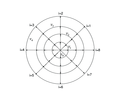
Figure 1: Sketch of the discrete-velocity-model used in the present paper.

It’s easy to prove that this DVM at least up to seventh rank isotropy. The evolution of the distribution function $f_{ki}$ with the Bhatanger-Gross-Krook approximation[24] reads,

$$\frac{\partial f_{ki}}{\partial t}+\mathbf{v}_{ki}\cdot\frac{\partial f_{ki}}{\partial\mathbf{r}}=-\frac{1}{\tau}\left[f_{ki}-f_{ki}^{eq}\right],$$ (2)

where $f_{ki}^{eq}$ is the discrete version of the local equilibrium distribution function; $\mathbf{r}$ is the spatial coordinate; $\tau$ is the relaxation time; the local particle density $n$, hydrodynamic velocity $\mathbf{u}$ and temperature $T$ are defined by

$$n=\sum_{ki}f_{ki}^{eq},$$ (3)

$$n\mathbf{u}=\sum_{ki}\mathbf{v}_{ki}f_{ki}^{eq},$$ (4)

$$P=e_{int}=nT=\sum_{ki}\frac{1}{2}(\mathbf{v}_{ki}-\mathbf{u})^{2}f_{ki}^{eq}$$ (5)

where $P$ and $e_{int\text{ }}$are the local pressure and internal energy. This model is designed to recover the following Navier-Stokes equations

$$\frac{\partial\rho}{\partial t}+\frac{\partial(\rho u_{\alpha})}{\partial r_{\alpha}}=0,$$ (6)

$$\frac{\partial(\rho u_{\alpha})}{\partial t}+\frac{\partial(\rho u_{\alpha}u_{\beta}+P\delta_{\alpha\beta})}{\partial r_{\beta}}-\frac{\partial}{\partial r_{\beta}}[\mu(\frac{\partial u_{\beta}}{\partial r_{\alpha}}+\frac{\partial u_{\alpha}}{\partial r_{\beta}}-\frac{\partial u_{\gamma}}{\partial r_{\gamma}}\delta_{\alpha\beta})]=0,$$ (7)

$$\frac{\partial}{\partial t}[\rho(e_{int}+\frac{u^{2}}{2})]+\frac{\partial}{\partial r_{\alpha}}[\rho u_{\alpha}(e_{int}+\frac{u^{2}}{2}+\frac{P}{\rho})]-\frac{\partial}{\partial r_{\alpha}}[\kappa^{{}^{\prime}}\frac{\partial e_{int}}{\partial r_{\alpha}}$$

$$+\mu u_{\beta}(\frac{\partial u_{\beta}}{\partial r_{\alpha}}+\frac{\partial u_{\alpha}}{\partial r_{\beta}}-\frac{\partial u_{\gamma}}{\partial r_{\gamma}}\delta_{\alpha\beta})]=0$$ (8)

in the hydrodynamic limit, where $\mu$ ,$\kappa^{{}^{\prime}}$ are viscosity coefficient and heat conductivity coefficient, having the following relations with pressure $P$ and relaxation time $\tau$ :

$$\mu=P\tau,\kappa^{{}^{\prime}}=2\mu\text{.}$$ (9)

The equilibrium distribution function $f_{ki}^{eq}$ is calculated in the following way,

$$f_{ki}^{eq} = nF_{k}[(1-\frac{u^{2}}{2\theta}+\frac{u^{4}}{8\theta^{2}})+\frac{v_{ki\varepsilon}u_{\varepsilon}}{\theta}(1-\frac{u^{2}}{2\theta})+\frac{v_{ki\varepsilon}v_{ki\pi}u_{\varepsilon}u_{\pi}}{2\theta^{2}}(1-\frac{u^{2}}{2\theta})]+$$ (10)

$$\frac{v_{ki\varepsilon}v_{ki\pi}v_{ki\vartheta}u_{\varepsilon}u_{\pi}u_{\vartheta}}{6\theta^{3}}+\frac{v_{ki\varepsilon}v_{ki\pi}v_{ki\vartheta}v_{ki\xi}u_{\varepsilon}u_{\pi}u_{\vartheta}u_{\xi}}{24\theta^{4}}]$$

with

$$F_{k} = \frac{1}{v_{k}^{2}(v_{k}^{2}-v_{k+1}^{2})(v_{k}^{2}-v_{k+2}^{2})(v_{k}^{2}-v_{k+3}^{2})}[48\theta^{4}-6(v_{k+1}^{2}+v_{k+2}^{2}+v_{k+3}^{2})\theta^{3}+$$ (11)

$$(v_{k+1}^{2}v_{k+2}^{2}+v_{k+2}^{2}v_{k+3}^{2}+v_{k+3}^{2}v_{k+1}^{2})\theta^{2}-\frac{v_{k+1}^{2}v_{k+2}^{2}v_{k+3}^{2}}{4}\theta]\text{,}$$

$$F_{0}=1-8(F_{1}+F_{2}+F_{3}+F_{4})\text{,}$$ (12)

and

$$\theta=\frac{T}{m}\text{,}$$

where

$$\left\{k+l\right\}=\left\{\begin{array}[]{ll}k+l&\text{ if }k+l\leq 4\\ k+l-4&\text{ if }k+l>4\end{array}\right.\text{.}$$ (13)

We choose $v_{0}=0$ and four nonzero $v_{k}(k=1,2,3,4)$.

3 Modified Lax-Wendroff scheme and artificial viscosity

To simplify the discussion, we work on the general Cartesian coordinate. The combination of the above DVM and the general FD scheme with first-order forward in time and second-order upwinding in space composes the original FDLB model by WT. It has been validated via the Couette flow, small Mach number Riemann problems. When the Mach number $M$ exceeds $1,$ the original LB model is not stable. The DVM is derived independent of Mach number. Therefore, we resort to the discretization of the left-hand side of Eq. (2) to make an accurate and stable LB scheme. Here we investigate a mixed scheme which is composed of a modified Lax-Wendroff[25] and an artificial viscocity.

As we know, the original Lax-Wendroff (LW) scheme is very dissipative and has a strong “smoothing effect”. Obviously, it is not favorable when needing capture shocks in the system. To compromise the accuracy and stability, we add a dispersion term and the artificial viscosity to the right-hand side of Eq. (2) before discretization so that we have

$$\frac{\partial f_{ki}}{\partial t}+v_{ki\alpha}\frac{\partial f_{ki}}{\partial r_{\alpha}} = -\frac{1}{\tau}\left[f_{ki}-f_{ki}^{eq}\right]+\frac{v_{ki\alpha}(1-c_{ki\alpha}^{2})\Delta r_{\alpha}^{2}}{6}\frac{\partial^{3}f_{ki}}{\partial r_{\alpha}^{3}}$$ (14)

$$+\theta_{\alpha I}\left|\kappa_{\alpha}\right|(1-\left|\kappa_{\alpha}\right|)\frac{\Delta r_{\alpha}^{2}}{2\Delta t}\frac{\partial^{2}f_{ki}}{\partial r_{\alpha}^{2}}\text{,}$$

where

$$c_{ki\alpha}=v_{ki\alpha}\Delta t/\Delta r_{\alpha}\text{, }\kappa_{\alpha}=u_{\alpha}\Delta t/\Delta r_{\alpha}\text{; }$$ (15)

$$\theta_{\alpha I}=\lambda\left|\frac{P_{\alpha I+1}-2P_{\alpha I}+P_{\alpha I-1}}{P_{\alpha I+1}+2P_{\alpha I}+P_{\alpha I-1}}\right|$$ (16)

plays a role of the switching function, $\lambda$ is a coefficient controlling the amplitude of the artificial viscosity. Using the Lax-Wendroff to the left-hand side and central difference to the right-hand side of Eq. (14) results in the following LB equation,

$$f_{kiI}^{new} = f_{kiI}-\frac{c_{ki\alpha}}{2}(f_{kiI+1}-f_{kiI-1})-\frac{\Delta t}{\tau}\left[f_{kiI}-f_{kiI}^{eq}\right]$$ (17)

$$+\frac{c_{ki\alpha}^{2}}{2}(f_{kiI+1}-2f_{kiI}+f_{kiI-1})$$

$$+\frac{c_{ki\alpha}(1-c_{ki\alpha}^{2})}{12}(f_{kiI+2}-2f_{kiI+1}+2f_{kiI-1}-f_{kiI-2})$$

$$+\frac{\theta_{\alpha I}\left|\kappa_{\alpha}\right|(1-\left|\kappa_{\alpha}\right|)}{2}(f_{kiI+1}-2f_{kiI}+f_{kiI-1})\text{,}$$

where the third suffixes $I-1,I,I+1$ indicate the mesh nodes in $x$ or $y$ direction. The positions of terms 3 and 4 in the right-hand side of Eq. (17) have been exchanged. It is clear that the first line corresponds to the general LB equation with the central difference in space; compared with the central difference, the Lax-Wendroff contributes an extra line II; lines III and IV show the added dispersion term and artificial viscosity.

4 von Neumann Stability Analysis

We analysis the numerical stability of the FDLBM by means of von Neumann stability analysis[21, 22]. In the analysis solution of finite-difference equation is written as the familiar Fourier series, and the numerical stability is evaluated by the magnitude of eigenvalues of an amplification matrix. The small perturbation $\Delta f_{ki}$ is defined as: $f_{ki}(\mathbf{r},t)=\Delta f_{ki}(\mathbf{r},t)+\bar{f_{ki}^{0}}$, where $\bar{f_{ki}^{0}}$ is the global equilibrium distribution function which is a constant, depends only on the mean density, velocity and temperature. From equation(14) we can obtain

$$\frac{\Delta f_{ki}(r_{\alpha},t+\Delta t)-\Delta f_{ki}(r_{\alpha},t)}{\Delta t}+v_{ki\alpha}\frac{\partial\Delta f_{ki}}{\partial r_{\alpha}}=-\frac{1}{\tau}\left[\Delta f_{ki}-\Delta f_{ki}^{eq}\right]$$

$$+\frac{v_{ki\alpha}(1-c_{ki\alpha}^{2})\Delta r_{\alpha}^{2}}{6}\frac{\partial^{3}\Delta f_{ki}}{\partial r_{\alpha}^{3}}+\theta_{\alpha I}\left|\kappa_{\alpha}\right|(1-\left|\kappa_{\alpha}\right|)\frac{\Delta r_{\alpha}^{2}}{2\Delta t}\frac{\partial^{2}\Delta f_{ki}}{\partial r_{\alpha}^{2}}\text{.}$$ (18)

The perturbation part $\Delta f_{ki}(r_{\alpha},t)$ may be written as series of complex exponents, $\Delta f_{ki}(r_{\alpha},t)=F_{ki}^{t}\mathrm{exp}(\mathbf{i}k_{\alpha}r_{\alpha})$, where $F_{ki}^{t}$ is an amplitude at grid point $r_{\alpha}$ and time $t$, $\mathbf{i}$ is an imaginary unit, and $k_{\alpha}$ is the wave number of sine wave in the domain with the highest resolution $1/\Delta r_{\alpha}$. Substituting this expansion into the equation (18), we obtain $F_{ki}^{t+\Delta t}=G_{ij}F_{kj}^{t}$ , where $G_{ij}$ is a matrix being used to assess amplification rate of $F_{ki}^{t}$ per time step $\Delta t$. If the maximum of the eigenvalues of the amplification matrix satisfies the condition, $\mathrm{max}|\omega|\leq 1$, for all wave numbers, the FD scheme is surely stable, where $\omega$ is the eigenvalue of the amplification matrix. This is the von Neumann condition for stability. The amplification matrix $G_{ij}$ can be written as following,

$$G_{ij} =\left(1-\frac{\Delta t}{\tau}\right)\delta_{ij}+\frac{\Delta t}{\tau}\frac{\partial f_{ki}^{eq}}{\partial f_{kj}}-\frac{c_{ki\alpha}}{2}(e^{\mathbf{i}k_{\alpha}\Delta r_{\alpha}}-e^{-\mathbf{i}k_{\alpha}\Delta r_{\alpha}})\delta_{ij}+\frac{c_{ki\alpha}^{2}}{2}(e^{\mathbf{i}k_{\alpha}\Delta r_{\alpha}}-2$$

$$+e^{-\mathbf{i}k_{\alpha}\Delta r_{\alpha}})\delta_{ij}+\frac{c_{ki\alpha}(1-c_{ki\alpha}^{2})}{12}(e^{\mathbf{i}2k_{\alpha}\Delta r_{\alpha}}-2e^{\mathbf{i}k_{\alpha}\Delta r_{\alpha}}+2e^{-\mathbf{i}k_{\alpha}\Delta r_{\alpha}}-e^{-\mathbf{i}2k_{\alpha}\Delta r_{\alpha}})\delta_{ij}$$

$$+\frac{\theta_{\alpha I}\left|\kappa_{\alpha}\right|(1-\left|\kappa_{\alpha}\right|)}{2}(e^{\mathbf{i}k_{\alpha}\Delta r_{\alpha}}-2+e^{-\mathbf{i}k_{\alpha}\Delta r_{\alpha}})\delta_{ij}\text{,}$$ (19)

$$\frac{\partial f_{ki}^{eq}}{\partial f_{kj}}=\frac{\partial f_{ki}^{eq}}{\partial\rho}\frac{\partial\rho}{\partial f_{kj}}+\frac{\partial f_{ki}^{eq}}{\partial T}\frac{\partial T}{\partial f_{kj}}+\frac{\partial f_{ki}^{eq}}{\partial u_{\alpha}}\frac{\partial u_{\alpha}}{\partial f_{kj}}\text{.}$$ (20)

Several researchers have analyzed the stability of the incompressible LB models[21, 26, 27], it is found that there is not a single wave-number being always the most unstable. For the 2D DVM by WT, $G_{ij}$ is a matrix with $33\times 33$ elements. Moreover, every element is related to the macroscopical variables (density, temperature, velocities), discrete velocities and other constants, so it is difficult to analyze with explicit expressions. We resort to using the software, Mathematica-5 to conduct a series of quantitative analysis. Now we show some numerical results of von Neumann analysis by Mathematica-5. The results will be shown by figures with curves for the maximum eigenvalue $|\omega|_{max}$ of $G_{ij}$ versus $k\Delta x$.

Figure 2 shows a comparison of the fours different cases, (i) LB with only the central-difference to the convection term, i.e. LB scheme based only on the first line of Eq. (17) (see the black line with squares); (ii) LB with Lax-Wendroff, i.e., LB scheme based on the first two lines of Eq. (17) (see the red line with circles); (iii) LB scheme based on lines 1 and 3 of Eq. (17) (see the green line with triangles); (iv) LB scheme based on the whole of Eq. (17) (see the blue line with triangles down). Here the macroscopic variables are chosen as $(\rho,u_{1},u_{2},T)$ = $(2.0,30.0,0.0,1.0)$, and the remaining parameters are $(v_{0},v_{1},v_{2},v_{3},v_{4})$ = $(0.0,1.0,1.92,2.99,4.49)$, $\lambda=0.5$, $\Delta x=\Delta y=3\times 10^{-3}$, $\Delta t=\tau=10^{-5}$. It is clear that the artificial viscosity term can significantly decrease the maximum eigenvalue $|\omega|_{\text{max}}$ from being larger than to be smaller than $1$ for appropriately given time step. Moreover, it is worthy to note that dissipation term in line 2 of Eq. (17) favors and dispersion term in line 3 disfavors the stability to some extent. Numerical experiments show that the dispersion term may effectively reduce numerical oscillations near discontinuity and improves the accuracy (see Fig. 3 for an example).

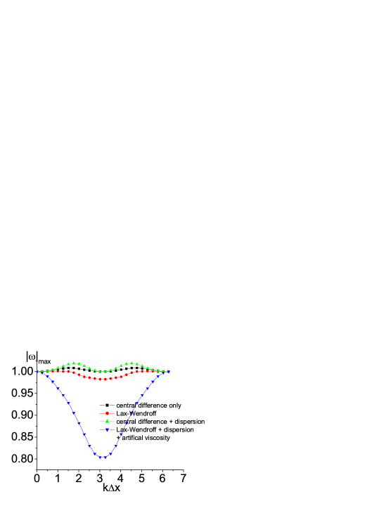
Figure 2: (Color online) Stability analysis for four conditions. The macroscopic variables are set as $(\rho,u_{1},u_{2},T)$ = $(2.0,30.0,0.0,1.0)$, the other constants are set as $(v_{0},v_{1},v_{2},v_{3},v_{4})$ = $(0.0,1.0,1.92,2.99,4.49)$, $\lambda=0.5$,$\Delta x=\Delta y=3\times 10^{-3}$,$\Delta t=$ $\tau$ $=10^{-5}$.

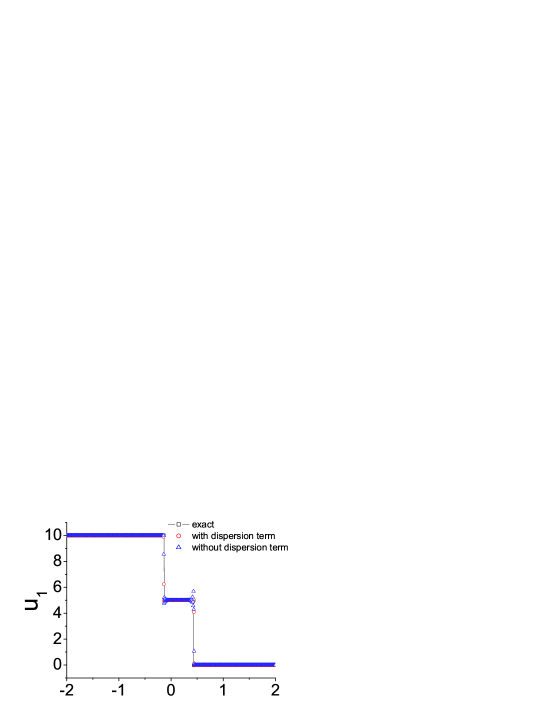
Figure 3: (Color online) Effects of dispersion to simulation. The macroscopic variables at two sides of a shock tube are set as $(\rho,u_{1},u_{2},T)|_{L}=(10.0,10.0,0.0,5.0)$, $(\rho,u_{1},u_{2},T)|_{R}=(10.0,0.0,0.0,5.0)$, $\lambda=2.0$. The other constants and macroscopic variables are the same as in Fig.2.

Figure 4 shows the effects of various artificial viscosities to the stability. Fig.(a) shows the cases with $\lambda=1.0$, $0.5$, $0.1$, and $0.05$. Fig.(b) shows the cases with $\lambda=1.0$, $1.8$,$2.0$, and $3.0$. The other constants and macroscopic variables are unchanged. From this figure we can see some relevance: Strength of artificial viscosity has a large impact on the stability. LB works only within a certain range of artificial viscosity. In practical simulations, we generally take the smaller viscosity in favor of the accuracy.

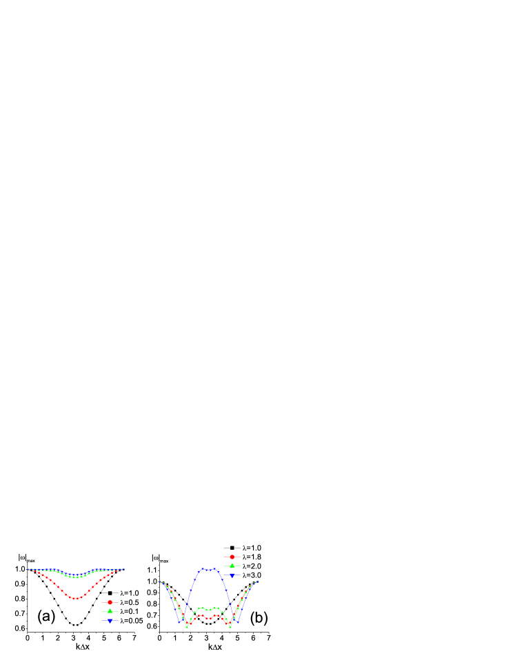
Figure 4: (Color online) Effects of various artificial viscosities to the numerical stability. Fig. (a) shows the cases with $\lambda=1.0$, $0.5$, $0.1$, $0.05$. Fig. (b) shows the cases with $\lambda=1.0$,$1.8$, $2.0$, $3.0$. The other constants and macroscopic variables are unchanged.

Since the density $\rho$ can be normalized to $1$, we then need only investigate the effects of the other two physical quantities, temperature $T$ and flow velocity $\mathbf{u}$. Figure 5 shows four cases with $T=1$, $T=5$, $T=15$ and $T=25$. Here $u_{1}=5$, $u_{2}=0$ and $\lambda=0$. When other parameters are fixed, the numerical stability becomes better with the increasing of temperature. This can also be understood that higher temperature corresponds to higher sound speed and lower Mach number.

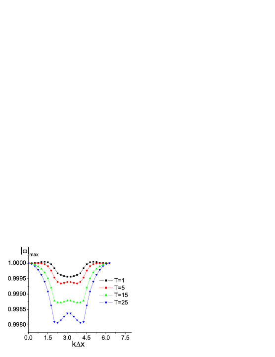
Figure 5: (Color online) Influence of temperature $T$ to numerical stability. $u_{1}=5$, $u_{2}=0$ and $\lambda=0$. The other physical quantities and model parameters are unchanged.

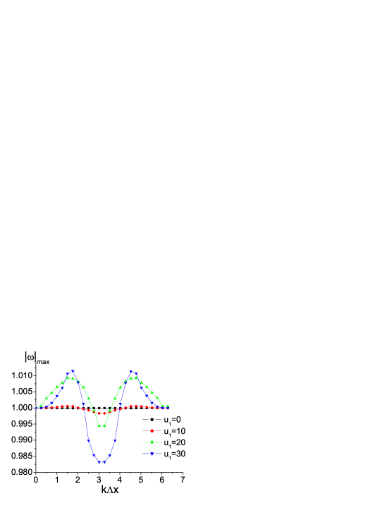
Figure 6: (Color online) Influence of velocity $\mathbf{u}$ to numerical stability. The value of $u_{1}$ is altered from zero to $30$ and $u_{2}=0$. Here $\lambda=0$, the other constants and macroscopic variables are unchanged.

Figure 6 shows cases with difference flow velocities. The value of $u_{1}$ is altered from zero to $30$ and $u_{2}=0$. Here $\lambda=0$, the other constants and macroscopic variables are unchanged. This figure clearly shows that the higher the Mach number, the larger the maximum eigenvalue, which answers why the numerical stability becomes worse with the increasing of Mach number of the fluid.

5 Numerical tests and analysis

In this section two kinds of typical benchmarks are used to validate the newly proposed scheme. The first kind is the Riemann problem[28]. The second one is the problem of shock reflection[29].

5.1 Riemann problems[28]

Here the two-dimensional model is used to solve the one-dimensional Riemann problem. The initial macroscopic variables at the two sides are denoted by $(\rho$, $u_{1}$, $u_{2}$, $T)|_{L}$ and $(\rho$, $u_{1}$, $u_{2}$, $T)|_{R}$, respectively.

5.1.1 Sod’s shock tube

For the problem considered, the initial condition is described by

$$\left\{\begin{array}[]{l}(\rho,u_{1},u_{2},T)|_{L}=(1.0,0.0,0.0,1.0)\\ (\rho,u_{1},u_{2},T)|_{R}=(0.125,0.0,0.0,0.8)\end{array}\right.$$ (21)

Figure 7 shows the computed density, pressure, velocity, temperature profiles at $t=0.2$, where the circles are simulation results and solid lines with squares are analytical solutions. The size of grid is $\Delta x=\Delta y=10^{-3}$, time step $\Delta t=10^{-5}$, and $\tau=$ $10^{-4}$, $\lambda=2.$ The two sets of results have a satisfying agreement.

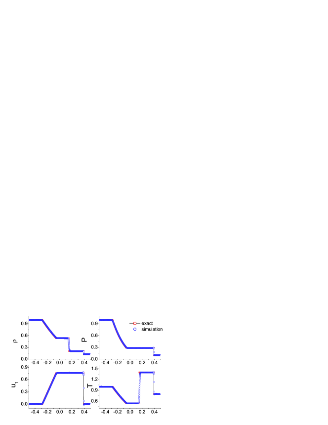
Figure 7: (Color online) Comparison of numerical and theoretical results for the Sod shock tube, where t=0.2. Solid lines with squares are for exact solutions and circles are for simulation results.

5.1.2 Lax’s shock tube

The initial condition of this problem reads

$$\left\{\begin{array}[]{l}(\rho,u_{1},u_{2},T)|_{L}=(0.445,0.698,0.0,7.928)\\ (\rho,u_{1},u_{2},T)|_{R}=(0.5,0.0,0.0,1.142)\end{array}\right.$$ (22)

Figure 8 shows the results at $t=0.2$, where the circles are simulation results and solid lines with squares correspond to exact solutions. The parameters are set to be $\Delta x=\Delta y=10^{-3}$, $\Delta t=10^{-5}$, $\tau=$ $10^{-4}$, and $\lambda=1$. We also find a good agreement between the two sets of results.

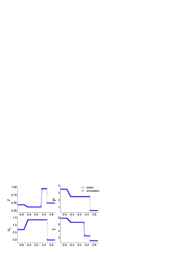
Figure 8: (Color online) Comparison of numerical and theoretical results for the Lax shock tube at $t=0.2$. Solid lines with squares are for exact solution and circles are for simulation results.

5.1.3 Sjogreen’s problem

The initial condition of this problem is

$$\left\{\begin{array}[]{l}(\rho,u_{1},u_{2},T)|_{L}=(1.0,-2.0,0.0,0.4)\\ (\rho,u_{1},u_{2},T)|_{R}=(1.0,2.0,0.0,0.4)\end{array}\right.$$ (23)

The numerical and exact solutions at $t=0.018$ are shown in Fig.9, where $\Delta x=\Delta y=3\times 10^{-3}$, $\Delta t=\tau=10^{-5}$ and $\lambda=1.8$. The exact solution of this problem consists of two strong rarefaction waves and a weak constant contact discontinuity. Pressure near the contact discontinuity is very small, which brings certain difficulties to simulation. Temperature and density calculated by many schemes are negative. However, the improved model ensures the positivity of them. Successful simulation of this problem proves that the improved model is applicable to the low-density, low-temperature flow simulations.

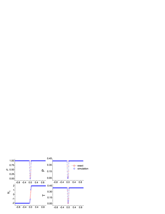
Figure 9: (Color online) Comparison of numerical and theoretical results for the Sjogreen problem at $t=0.018$. Solid lines with squares are for exact solutions, and circles are for simulation results.

5.1.4 Colella’s explosion wave problem

The initial condition of this test can be write as

$$\left\{\begin{array}[]{l}(\rho,u_{1},u_{2},T)|_{L}=(1.0,0.0,0.0,1000.0)\\ (\rho,u_{1},u_{2},T)|_{R}=(1.0,0.0,0.0,0.01)\end{array}\right.$$ (24)

This is generally regarded as a difficult test. The exact solution contains a leftwards rarefaction wave, a contact discontinuity and a strong shock. It is generally used to check the robustness and accuracy. Figure 10 gives comparison of the numerical and theoretical results at $t=0.05$. Here $\lambda=20$, other parameters are same as in the Sjogreen test. Successful simulation of this test proves the improved model is applicable to flows with very high ratios of temperature and pressure.

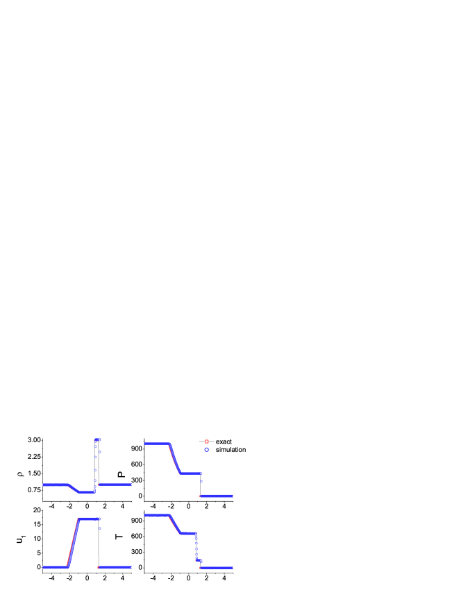
Figure 10: (Color online) Comparison of numerical and theoretical results for the Colella explosion wave problem at t=0.05. Solid lines with squares are for exact solutions and circles are for simulation results.

5.1.5 Collision of two strong shocks

This test with the following initial data:

$$\left\{\begin{array}[]{l}(\rho,u_{1},u_{2},T)|_{L}=(5.99924,19.5975,0.0,76.8254)\\ (\rho,u_{1},u_{2},T)|_{R}=(5.99242,-6.19633,0.0,7.69222)\end{array}\right.$$ (25)

This is also a difficult test. Exact solution contains a leftwards shock, a right contact discontinuity and shock which spreading to right side. And the left-shock spreads to right very slowly, which brings additional difficulties to the numerical method. Fig.11 gives a comparison of the numerical and theoretical results at $t=0.12$. Parameters used in this test are $\Delta x=\Delta y=2\times 10^{-3}$, $\Delta t=\tau=10^{-5}$ and $\lambda=1$. The good agreement between the two sets of results shows again the robustness of the improved model.

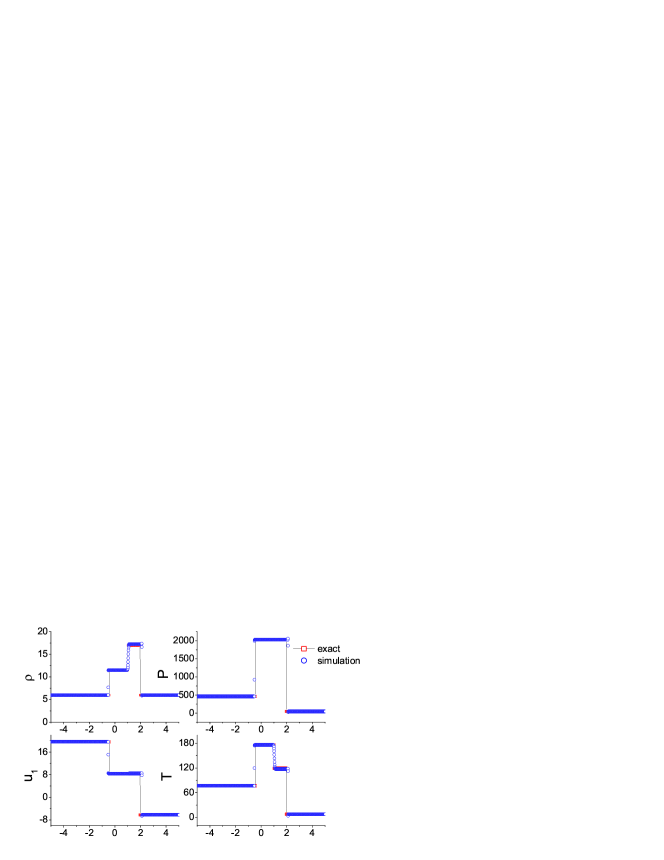
Figure 11: (Color online) Comparison of numerical and theoretical results for collision of two strong shocks at $t=0.12$. Solid lines with symbols are for exact solutions and symbols are for simulation results.

5.2 Shock reflections[29]

We will present two gas dynamics simulations. Both are done on rectangular grid. The first is to recover a steady regular shock reflection. The second is the double Mach reflection of a shock off an oblique surface. This example is used in Ref.[30] as a benchmark test for comparing the performance of various difference methods on problem involving strong shocks.

5.2.1 Steady regular shock reflection

In the first test problem, the incoming shock wave with Mach number 20 has an angle of $30^{\circ}$ to the wall. The computational domain is a rectangle with length $0.9$ and height $0.3$. This domain is divided into a $300\times 100$ rectangular grid with $\Delta x=\Delta y=0.003$. The boundary conditions are composed of a reflecting surface along the bottom boundary, supersonic outflow along the right boundary , and Dirichlet conditions on the left and top boundary conditions, given by

$$\left\{\begin{array}[]{l}(\rho\text{, }u_{1}\text{, }u_{2}\text{, }T)|_{0\text{, }y\text{, }t}=(1.0\text{, }20.0\text{, }0.0\text{, }0.5)\text{,}\\ (\rho\text{, }u_{1}\text{, }u_{2}\text{, }T)|_{x\text{, }0.3\text{, }t}=(\frac{50}{17}\text{, }16.7\text{, }-5.71578\text{, }22.61)\text{.}\end{array}\right.$$ (26)

Figure 12 shows contours of density at $t=0.2$. The clear shock reflection on the wall agrees well with the exact solution.

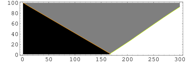
Figure 12: (Color online)Density contour of steady regular shock reflection on a wall at t=0.2. From black to white, the density increases.

5.2.2 Double Mach reflection

In this test, we considered an unsteady shock reflection. The initial pressure ratio here is high. A planar shock is incident towards an oblique surface with a $30^{\circ}$ angle to the direction of propagation of the shock. A uniform mesh size of $500\times 200$ is used for the numerical simulation. The conditions for both sides are:

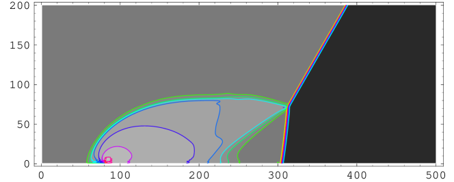
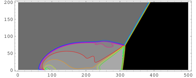
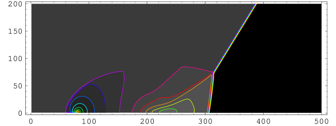
Figure 13: (Color online) Contours of density (top), temperature (center), and $u_{1}$ (bottom) of the double Mach reflection problem at the 750th iteration step. The units of the $x$- and $y$- axes are both $0.001$.

$$\left(\rho,u_{1},u_{2},T\right)\mid_{x\text{,}y\text{,}0}=\left\{\begin{array}[]{ll}(\frac{400}{67},13.3\cos 30^{\circ},-13.3\sin 30^{\circ},89.2775),&\text{ if }y\geq h(x,0)\\ (2.0,0.0,0.0,0.5)&\text{ if }y<h(x,0)\end{array}\right.\text{,}$$ (27)

where $h(x,t)=\sqrt{3}(x-80\Delta x)-40t$. The reflecting wall lines along the bottom of the problem domain, beginning at $x=0.08.$ The shock makes a $60^{\circ}$ angle with the $x$ axis and extends to the top of the problem domain at $y=0.2.$ At the top boundary, the physical quantities are assigned the same values as on the left side for $x\leq g(t)$ and are assigned the same values on the right side, where $g(t)=80\Delta x+\sqrt{3}/3(0.2+40t)$. The computed density, temperature and flow velocity along the $x$-direction are shown in Fig.13, where complex characteristics, such as oblique shocks and triple points, are well captured.

6 Conclusions and discussions

A lattice Boltzmann model to the high-speed compressible Navier-Stokes system is presented. The new LB model is composed of the following components: the original DVM by Watari and Tsutahara, a modified Lax-Wendroff scheme and an additional artificial viscosity. Compared with the central difference scheme, the Lax-Wendroff contributes a dissipation term which is in favor of the numerical stability, even though it is generally still not enough for high-speed flows. The introducing of the third-order dispersion term helps to eliminate some unphysical oscillations at discontinuity. The additional artificial viscosity compensates the insufficiency of the above-mentioned dissipation so that the LB simulation can continue smoothly. The adding of the dispersion and artificial viscosity terms should survive the dilemma of stability versus accuracy. In other words, they should be minimal but make the evolution satisfy the von Neumann stability condition. Due to the complexity, the analysis resorts to the software, Mathematica-5, and only some typical results are shown by figures.

Typical benchmark tests are used to validate the proposed scheme. Riemann problems, including the Sod, Lax, Sjogreen, Colella explosion wave, collision of two strong shocks, show good accuracy and numerical stability of the new scheme, even though they are generally difficult to resolve by traditional computational fluid dynamics[28, 29, 30, 31]. Regular and double Mach shock reflections are successfully recovered. These simulations show that the improved LB model may be used to investigate some long-standing problems, such as the transitions between regular and Mach reflections. By incorporating an appropriate equation of state, or equivalently, a free energy functional, or an external force, the present model may be used to simulate liquid-vapor transition and relevant flow behavior. Future work includes a more complete description of the problem on numerical accuracy versus stability and thermal lattice Boltzmann model for multi-phase flows.

References

- [1] S. Succi, The Lattice Boltzmann Equation for Fluid Dynamics and Beyond Oxford University Press, New York,2001.
- [2] Q. F. Wu, W. F. Chen, DSMC method for heat chemical nonequilibrium flow of high temperature rarefied gas, (in Chinese), National Defence Science and Technology University Press, Beijing (1999).
- [3] Aiguo Xu, X.F.Pan, Guangcai Zhang, and Jianshi Zhu, J. Phys.: Condens. Matter 19, 326212 (2007); J. Phys. D: Appl. Phys. (accepted for publication); Commun. Theor. Phys. (accepted for publication).
- [4] F. J. Alexander, H . Chen, S. Chen and G. D. Doolen, Phys. Rev. A 46, 1967 (1992).
- [5] Gangwu Yan, Yaosong Chen, Shouxin Hu, Phys. Rev. E. 59, 454(1999);
- [6] H. Yu and K. Zhao, Phys. Rev. E 61, 3867 (2000).
- [7] C. Sun, Phys. Rev. E 58, 7283 (1998).
- [8] C. Sun, Phys. Rev. E 61, 2645 (2000).
- [9] C. Sun and A. T. Hsu, Phys. Rev. E 68, 016303 (2003).
- [10] T. Kataoka and M. Tsutahara, Phys. Rev. E 69, 035701(R) (2004);Phys. Rev. E 69, 056702 (2004).
- [11] M. Watari and M. Tsutahara, Phys. Rev. E 67, 036306 (2003); Phys. Rev. E 70, 016703 (2004).
- [12] Aiguo Xu, Europhys. Lett. 69, 214 (2005); Phys Rev E 71, 066706 (2005); Prog. Theore.Phys.(Suppl.)162, 197 (2006).
- [13] R. Benzi, S. Succi, and M. Vergassola, Phys. Rep. 222, 145 (1992); D. A. Wolf-Gladrow, Lattice gas cellular automata and lattice Boltzmann models, Springer-Verlag, New York (2000); H. Chen, S. Kandasamy, S. Orszag, R. Shock, S. Succi, and V. Yakhot, Science 301, 633 (2003).
- [14] W. A. Yong and L. S. Luo, Phys. Rev. E. 67, 1063(2003).
- [15] A. Xiong, Acta Mech. Sinica (English Series) 18, 603 (2002).
- [16] F. Tosi, S. Ubertini, S. Succi, H. Chen, I.V. Karlin, Math. Comput. Simulat. 72, 227(2006)
- [17] S. Ansumali, I. V. Karlin, J. Stat. Phys. 107, 291(2002); S. Ansumali, I. V. Karlin, H. C. Ottinger, Europhys. Lett. 63, 798(2003)
- [18] Y. Li, R. Shock, R. Zhang, H. Chen, J. Fluid Mech. 519, 273(2004)
- [19] V. Sofonea, A. Lamura, G. Gonnella, A. Cristea, Phys. Rev. E 70 046702 (2004).
- [20] R. A. Brownlee, A. N. Gorban and J. Levesley, Phys. Rev. E. 75, 036711 (2007)
- [21] T. Seta and R. Takahashi, J. Stat. Phys. 107, 557 (2002).
- [22] X.F.Pan, Aiguo Xu, Guangcai Zhang, Song Jiang, Int. J. Mod. Phys. C (to be published); Preprint Version: arXiv:0706.0405vl.
- [23] Aiguo Xu, G. Gonnella, and A. Lamura, Phys. Rev. E 74 011505(2006); Phys. Rev. E 67, 056105 (2003); Physica A 331, 10 (2004); Physica A 344, 750 (2004); Physica A 362, 42 (2006); Aiguo Xu, Commun. Theor. Phys. 39, 729 (2003).
- [24] P. Bhatnagar, E. P. Gross, and M. K. Krook, Phys. Rev. 94, 511 (1954).
- [25] R. Liu and Q. Shu, Some New Methods in Computational Fluid Dynamics(in Chinese), Science Press, Beijing 2003.
- [26] J. D. Sterling and S. Chen, J. Comput. Phys. 123, 196 (1996).
- [27] X. D. Niu, C. Shu, Y. T. Chew, and T. G. Wang, J. Stat. Phys. 117, 665 (2004).
- [28] G. Lv, Advances in the study of the finite-Point Methods (in Chinese), Research Report of China Academy of Engineering Physics, Beijing 2006.
- [29] H. Zhang, Research on High Order Accurate Numerical Methods for Fluid Dynamics (in Chinese), Ph.D theses of Nanjing University of Aeronautics and Astronautics, Nanjing, 2005.
- [30] P. R. Woodward and P. Colella, J. Comput. Phys. 54, 115(1984).
- [31] Xijun Yu and Qingfang Dai, Numer. Methods for Part. Diff. Equat.22, 1455 (2006); Qingfang Dai and Xijun Yu, SIAM J. Sci. Comput. 28, 805 (2006).