Fluctuation theorem and large deviation function
for a solvable model of a molecular motor

Abstract

We study a discrete stochastic model of a molecular motor. This discrete model can be viewed as a minimal ratchet model. We extend our previous work on this model, by further investigating the constraints imposed by the Fluctuation Theorem on the operation of a molecular motor far from equilibrium. In this work, we show the connections between different formulations of the Fluctuation Theorem. One formulation concerns the generating function of the currents while another one concerns the corresponding large deviation function, which we have calculated exactly for this model. A third formulation concerns the ratio of the probability of observing a velocity $v$ to the same probability of observing a velocity $-v$. Finally, we show that all the formulations of the Fluctuation Theorem can be understood from the notion of entropy production.

I introduction

The living cell has evolved a diverse array of proteins, which can perform a variety of chemical functions. These proteins catalyze chemical reactions, control key processes like recognition or signalling, or act as molecular machines. Biological systems containing these elements are typically described as active because they are in a non-equilibrium state as opposed to non-active systems which can be considered at thermal equilibrium. Recently there has been a lot of interest in the non-equilibrium properties of active biological systems, such as the hair bundle of the ear Martin et al. (2001); Camalet et al. (2000), active membranes Manneville et al. (2001), active gels Kruse et al. (2003), active networks Mizuno et al. (2007), active lipid clusters Mayor and Rao (2004) and living cells Lau et al. (2003)…

Clearly, one step towards understanding active biological systems, starts with the understanding of single active proteins, such as for instance molecular motor proteins. These molecular motor are nano-machines that convert chemical energy derived from the hydrolysis of ATP into mechanical work and motion Howard (2001); Asbury (2005). Important examples include kinesin, myosin, RNA polymerase, and the $F_{0}/F_{1}$ rotating motor. Mechano-transduction (i.e., the process of conversion of chemical energy into mechanical work) in motors has been described theoretically by ratchet-models Jülicher et al. (1997); Parmeggiani et al. (1999), which rely on the fruitful concept of broken symmetry. According to the Curie principle, directed motion requires to break the spatial symmetry and the time reversal symmetry associated with equilibrium (detailed balance). The spatial symmetry is broken by the asymmetric interaction between the motor and the filament, while the time reversal symmetry is broken by chemical transitions, which break locally the detailed balance condition. From the continuous ratchet models described by Langevin equations Jülicher et al. (1997), it is possible to construct discrete stochastic models of molecular motors by considering only localized discrete transitions as explained in Ref. Kolomeisky and Widom (1998). These discrete stochastic models are interesting because they are minimal, in the sense that they contain the main physical picture of ratchet models while being more amenable to precise mathematical analysis Fisher and Kolomeisky (1999); Kafri et al. (2004); Jarzynski and Mazonka (1999); Lipowsky (2000).

Recent advances in experimental techniques to probe the fluctuations of single motors provide ways to gain insight into their kinetic pathways Schnitzer and Block (1997); Coppin et al. (1997); Carter and Cross (2005); Shaevitz et al. (2005). However, a general description for fluctuations of systems driven out of equilibrium, and in particular of motors, is still lacking. Recently, the Fluctuation Theorem (FT) has emerged as a promising framework to characterize fluctuations in far-from-equilibrium regimes. This theorem is in fact a group of closely related results valid for a large class of non-equilibrium systems Evans et al. (1993); Gallavotti (1996); Lebowitz and Spohn (1999); Evans and Searles (2002); Crooks (2000). In a nutshell, FT states that the probability distribution for the entropy production rate obeys a symmetry relation. The Theorem becomes particulary relevant for small systems in which fluctuations are large. For this reason, the FT has been verified in a number of beautiful experiments with small systems such as biopolymers and colloidal systems Liphardt et al. (2002). In the specific case of molecular motors, FT leads to constraints on the operation of molecular motors or nano-machines far from equilibrium in a regime where the usual thermodynamic laws do not apply Qian (2005); Gaspard and Gerritsma (2007); Seifert (2005).

In a recent work Lau et al. (2007), we have extended a two-states discrete stochastic model introduced in Ref. Kafri et al. (2004) by including an important variable, namely the number of ATP consumed. We have shown that this extended model satisfies FT, and we have constructed a thermodynamic framework allowing us to characterize quantities like the average velocity, the average ATP consumption rate and its thermodynamic efficiency. We have also analyzed the different thermodynamic modes of operation of the motor as functions of generalized forces arbitrarily far from equilibrium. Using FT, we have quantified the ”violations” of Einstein and Onsager relations. The deviations from Einstein and Onsager relations can be studied by considering the linear response theory in the vicinity a non-equilibrium steady state rather than near an equilibrium steady state. After determining the parameters of our model by a fit of single molecule experiments with kinesin Schnitzer and Block (1997), we have formulated a number of theoretical predictions for the ”violations” of Einstein and Onsager relations for this motor.

In this paper, we further extend the analysis of this model. In particular, we provide a more detailed study of the modes of operation of the motor and its thermodynamic efficiency in relation with the experimental data of kinesin. This part contains important information which could not be presented in Ref. Lau et al. (2007) due to limited space. The rest of the paper is devoted to bringing together different formulations of FT, explaining their connections and their physical implications. One way to formulate FT involves the generating function of the currents. We show that this formulation leads to two versions of FT, a long time version of FT similar to the Gallavotti-Cohen relation which holds quite generally, and a finite time version which is analogous to the Crooks-Evans transient Fluctuation Theorem Crooks (2000); Evans and Searles (2002) which holds under restricted hypotheses for the initial state. Another formulation of FT takes the form of a property of the large deviation function of the current. There are very few non-equilibrium models for which the large deviation function of the current is known exactly. Our model is sufficiently simple for this analytical calculation to be possible, and by carrying it out we show that the large deviation function of the current satisfies indeed an FT relation. A by-product of this calculation is a third formulation of FT in terms of the ratio of probabilities for observing a velocity $v$ to the same probability for observing a velocity $-v$. The prediction of this ratio of probabilities, which is obtained from the large deviation function of the current is one of the main results of this paper. We also study the connections between FT and the notion of entropy production. This entropy production can be explicitly calculated using the notion of affinities associated with a cyclic evolution of the mechanical and chemical variables, and the affinities precisely enter all the formulations of FT. We show that the entropy production can also be obtained from an evaluation of a quantity called the action functional Lebowitz and Spohn (1999). The entropy production and therefore also FT depends on the coarse-graining of the description which we illustrate by considering three different levels of description: purely mechanical, purely chemical and a combination of the two.

The paper is organized as follows: In Section II, we introduce the model, in Section III we consider the modes of operation of the motor, its thermodynamic efficiency and the comparison of the model with experimental data for kinesin. Section IV is devoted to the formulation of FT in terms of generating functions, with its long time and its finite time versions, Section V discusses the formulation in terms of the large deviation function of the current and the significance of the third formulation of FT in terms of a ratio of probabilities, and the last section contains the discussion of the entropy production.

II A two-state model for molecular motors

II.1 Construction of the model

Figure 1: A schematic of the rates for this two-state stochastic model of a single processive molecular motor. The position of the motor is $n$ and $y$ is the number of ATP consumed. The even and odd sites are denoted by $a$ and $b$, respectively. In the case of two headed kinesin, site $a$ represents a state where both heads are bound to the filament, whereas site $b$ represents a state with only one head bound. Note that the lattice of a and b sites extend indefinitely in both directions along the $n$ and $y$ axis. All the possible transitions are represented with arrows on this particular section of the lattice.

Figure 2: Cycles associated with the evolution of the motor of Fig. 1. Left: cycle for the position variable $n$; the average length $n$ undergone by the motor corresponds to half the number of full turns of the clock (the factor half is due to the period being equal to two lattice units) and with the rates as shown. Right: cycle for the chemical variable $y$, the average number of ATP units corresponds to the number of full turns with the rates shown. The affinities associated with these cycles are given by Eq. 11 for the mechanical variable and by Eq. 73 for the chemical variable.

As a result of conformational changes powered by hydrolysis of ATP, a linear processive motor, like kinesin, moves along a one-dimensional substrate (microtubule). The state of the molecular motor may be characterized by two variables: its position and the number of ATP consumed. To model the dynamics, we consider a linear discrete lattice, where the motor “hops” from one site to neighboring sites, either consuming or producing ATP (see Fig. 1). An alternate representation of the dynamics can be built in terms of cycles (see Fig. 2). The position is denoted by $x=nd$, where $2d\approx 8\,\mbox{nm}$ is the step size for kinesin. The even sites (denoted by $a$) are the low-energy state of the motor, whereas the odd sites (denoted by $b$) are its high-energy state; their energy difference is $\Delta E\equiv k_{B}T\epsilon$, where $k_{B}$ is the Boltzmann constant and $T$ is the temperature. This model is suitable to describe a two-headed kinesin walking on a microtubule, with the high-energy state corresponding to the state where a single head is bound to the filament, and the low-energy state corresponding to the two heads bound to it. Because of the periodicity of the filament, all the even ($a$) sites and all the odd ($b$) sites are equivalent.

The dynamics of the motor is governed by a master equation for the probability, $P_{i}(n,y,t)$, that the motor, at time $t$, has consumed $y$ units of ATP and is at site $i$ $(=a,b)$ with position $n$:

$$\partial_{t}P_{i}(n,y,t)=-\left(\overleftarrow{\omega}_{i}+\overrightarrow{\omega}_{i}\right)P_{i}(n,y,t)+\phantom{\overleftarrow{\omega}_{n+1}^{\,l}ppppppp}$$

$$\sum_{l=-1,0,1}\left[\,\overleftarrow{\omega}_{j}^{\,l}\,P_{j}(n+1,y-l,t)+\overrightarrow{\omega}_{j}^{\,l}\,P_{j}(n-1,y-l,t)\,\right],$$ (1)

with $i\neq j$, $\overleftarrow{\omega}_{j}\equiv\sum_{l}\overleftarrow{\omega}_{j}^{\,l}$ and $\overrightarrow{\omega}_{j}\equiv\sum_{l}\overrightarrow{\omega}_{j}^{\,l}$. We denote by $\overleftarrow{\omega}_{j}^{\,l}$ and $\overrightarrow{\omega}_{j}^{\,l}$ the transition rates from a site $j$ to a neighboring site to the left or to the right, respectively, and with $l\,(=-1,0,1)$ ATP molecules consumed. Note that the index $i$ is directly linked with the parity of $n$. We expect the rates $\overleftarrow{\omega}_{j}^{\,l}$ and $\overrightarrow{\omega}_{j}^{\,l}$ to be different even if no load is applied to the motor, because the interaction between the motor and the filament breaks the left-right (spatial) symmetry. This requirement is essential for generating directed motion.

Another essential requirement for generating directed motion is to break time-reversal symmetry. Such a symmetry is always present at equilibrium, where the detailed balance condition holds. Detailed balance is broken in molecular motors due to chemical transitions involved in the mechano-transduction process. To obtain a simple description of this process, we assume that transitions between the two states $\mbox{M}_{a}$ and $\mbox{M}_{b}$ of the motor Parmeggiani et al. (1999) are possible via two different chemical pathways:

$${{{\mathrm{M}_{\vphantom{}a}^{\vphantom{}\vphantom{\smash[t]{2+}}}}}+{}{{\mathrm{ATP}}}{{}\mathrel{\hbox to0.0pt{\raisebox{0.94722pt}{$\ext@arrow 3399\arrowfill@\relbar\relbar\rightharpoonup{\hphantom{\alpha_{b}}}{{\alpha_{a}}}$}\hss}\raisebox{-0.94722pt}{$\ext@arrow 3399\arrowfill@\leftharpoondown\relbar\relbar{\alpha_{b}}{\hphantom{{\alpha_{a}}}}$}}{}}{{\mathrm{M}_{\vphantom{}b}^{\vphantom{}\vphantom{\smash[t]{2+}}}}}+{}{{\mathrm{ADP}}}+{}{{\mathrm{P}}}},$$ (2)

and

$${{{\mathrm{M}_{\vphantom{}a}^{\vphantom{}\vphantom{\smash[t]{2+}}}}}{{}\mathrel{\hbox to0.0pt{\raisebox{0.94722pt}{$\ext@arrow 3399\arrowfill@\relbar\relbar\rightharpoonup{\hphantom{\beta_{b}}}{{\beta_{a}}}$}\hss}\raisebox{-0.94722pt}{$\ext@arrow 3399\arrowfill@\leftharpoondown\relbar\relbar{\beta_{b}}{\hphantom{{\beta_{a}}}}$}}{}}{{\mathrm{M}_{\vphantom{}b}^{\vphantom{}\vphantom{\smash[t]{2+}}}}}},$$ (3)

where $\alpha_{a}$ (resp. $\alpha_{b}$) are forward (resp. backward) rates. The first pathway ($\alpha$) represents transitions of the motor accompanied by ATP hydrolysis, which we call ”active”, and the second pathway ($\beta$) represents transitions driven by thermal activation, which we call ”passive”. In the representation of fig. 1, the $\alpha$-pathway represents oblique transitions which change both $y$ and $n$ whereas the $\beta$-pathway is associated with horizontal transitions which change only $n$. It is straightforward to generalize the model with more chemical pathways, but here we focus only on these two Parmeggiani et al. (1999). In the absence of an external force, transition state theory of chemical reactions requires that Hill (1987); De Donder (1927)

$$\frac{\alpha_{a}}{\alpha_{b}}=e^{-\epsilon+\Delta\mu},$$ (4)

and

$$\frac{\beta_{a}}{\beta_{b}}=e^{-\epsilon}.$$ (5)

Taking $\alpha_{a}=\overrightarrow{\omega_{a}}^{1},\alpha_{b}=\overleftarrow{\omega_{b}}^{-1},\beta_{a}=\overrightarrow{\omega_{a}}^{0},\beta_{b}=\overleftarrow{\omega_{b}}^{0}$ and $\alpha_{a}=\overleftarrow{\omega_{a}}^{1},\alpha_{b}=\overrightarrow{\omega_{b}}^{-1},\beta_{a}=\overleftarrow{\omega_{a}}^{0},\beta_{b}=\overrightarrow{\omega_{b}}^{0}$, we construct the transition rates from only four unknown parameters $\alpha$, $\alpha^{\prime}$, $\omega$ and $\omega^{\prime}$ as follows,

$$\begin{array}[]{ll}\overleftarrow{\omega_{b}}^{-1}=\alpha\,,&\overleftarrow{\omega_{b}}^{0}=\omega\,,\\ \overrightarrow{\omega_{a}}^{1}=\alpha\,e^{-\epsilon+\Delta\mu},&\overrightarrow{\omega_{a}}^{0}=\omega\,e^{-\epsilon},\\ \overleftarrow{\omega_{a}}^{1}=\alpha^{\prime}e^{-\epsilon+\Delta\mu},&\overleftarrow{\omega_{a}}^{0}=\omega^{\prime}\,e^{-\epsilon},\\ \overrightarrow{\omega_{b}}^{-1}=\alpha^{\prime},&\overrightarrow{\omega_{b}}^{0}=\omega^{\prime}\,,\end{array}$$ (6)

and with $\overleftarrow{\omega_{b}}^{1}=\overrightarrow{\omega_{a}}^{-1}=\overleftarrow{\omega_{a}}^{-1}=\overrightarrow{\omega_{b}}^{1}=0$. The only thermodynamic force driving the chemical cycle is the free energy of hydrolysis. This is quantified by the chemical potential $\Delta\widetilde{\mu}\equiv k_{B}T\Delta\mu$, which is defined by the standard expression not (a)

$$\Delta\tilde{\mu}=k_{B}T\ln\left(\frac{[ATP]\,[ADP]_{eq}\,[P]_{eq}}{[ATP]_{eq}\,[ADP]\,[P]}\right),$$ (7)

where $[..]$ denotes concentration under experimental conditions and $[..]_{eq}$ denotes equilibrium concentrations. The chemical potential of the hydrolysis reaction introduces a bias in the dynamics of the motor, which is responsible for breaking the time-reversal symmetry associated with the detailed balance condition (which holds at equilibrium).

Following Ref. Fisher and Kolomeisky (1999), the transition rates can be generalized to include an external force $F_{e}$ according to $\overleftarrow{\omega}_{i}^{\,l}(F_{e})=\overleftarrow{\omega}_{i}^{\,l}(0)\,e^{-\theta^{-}_{i}f}$ and $\overrightarrow{\omega}_{i}^{\,l}(F_{e})=\overrightarrow{\omega}_{i}^{\,l}(0)\,e^{+\theta^{+}_{i}f}$, where $f\equiv F_{e}d/(k_{B}T)$ and $\theta^{\pm}_{i}$ are the load distribution factors. These load distribution factors take into account the fact that the external force may not distribute uniformly among different transitions Hill (1987). Thus, we may write the non-zero rates in the presence of force as:

$$\begin{array}[]{ll}\overleftarrow{\omega_{b}}^{-1}=\alpha\,e^{-\theta^{-}_{b}f},&\overleftarrow{\omega_{b}}^{0}=\omega\,e^{-\theta^{-}_{b}f},\\ \overrightarrow{\omega_{a}}^{1}=\alpha\,e^{-\epsilon+\Delta\mu+\theta^{+}_{a}f},&\overrightarrow{\omega_{a}}^{0}=\omega\,e^{-\epsilon+\theta^{+}_{a}f},\\ \overleftarrow{\omega_{a}}^{1}=\alpha^{\prime}e^{-\epsilon+\Delta\mu-\theta^{-}_{a}f},&\overleftarrow{\omega_{a}}^{0}=\omega^{\prime}\,e^{-\epsilon-\theta^{-}_{a}f},\\ \overrightarrow{\omega_{b}}^{-1}=\alpha^{\prime}e^{\theta^{+}_{b}f},&\overrightarrow{\omega_{b}}^{0}=\omega^{\prime}\,e^{\theta^{+}_{b}f}\,.\end{array}$$ (8)

In the above expressions, the values of the parameters $\theta_{i}^{\pm}$ are arbitrary except for the following constraint: After one period, the work done by $F_{e}$ on the motor is $-F_{e}2d$, implying that $\theta^{+}_{a}+\theta^{-}_{b}+\theta^{-}_{a}+\theta^{+}_{b}\ =2$. Indeed, as shown in fig 4, the simplest model with all the $\theta_{i}^{\pm}$’s equal to $1/2$, which was studied in Ref. Kafri et al. (2004), does not reproduce the experimental curves of velocity versus force for kinesin. The fact that the $\theta_{i}^{\pm}$’s are different from 1/2 agrees with standard models of kinesin, in which several chemical transitions are involved, and the force must be split unequally among the different transition rates Howard (2001). We note that this splitting of the force (which involves the actual value of the $\theta_{i}^{\pm}$’s) is a matter of kinetics, whereas thermodynamics enforces only Eqs. 4-5. The expression of the rates given in Eqs. 6-8 is essential for the analysis which we develop below: we emphasize that these expressions are based on first principles. Once these rates are decomposed into an active and a passive part, the ratio of the passive transition rates in Eq. 5 follows from the condition of micro-reversibility (detailed balance), while the ratio of the active transition rates in Eq. 4 requires a more general principle for non-equilibrium chemical reactions. Such a principle is based on the notion of affinity, introduced by de Donder in Ref. De Donder (1927) to characterize non-equilibrium chemical reactions. The de Donder equation relates the forward and the backward reactions rates $\overrightarrow{\alpha}$ and $\overleftarrow{\alpha}$ of an elementary step, as a consequence of transition state theory:

$$\frac{\overrightarrow{\alpha}}{\overleftarrow{\alpha}}=e^{A/k_{B}T},$$ (9)

where $A$ is the affinity, defined as $-(\partial G/\partial\zeta)_{T,P}$ in terms of the Gibbs free energy $G$ and $\zeta$ the extend of reaction. At equilibrium, $A=0$ and Eq. 9 leads to $\overrightarrow{\alpha}=\overleftarrow{\alpha}$, which is the principle of micro-reversibility. Note that Eq. 4 is indeed of the form of Eq. 9, with the choice $\overrightarrow{\alpha}=\alpha_{a}$, $\overleftarrow{\alpha}=\alpha_{b}$ and $\Delta\mu=A/k_{B}T$ when $\epsilon=0$. Thus we can consider Eq. 4 as a De Donder relation, which generalizes the condition of micro-reversibility far from equilibrium De Donder (1927). Equivalently one can also interpret this equation as a particular case of generalized steady state balance conditions, we shall come back to this point in section IV.

II.2 Effective description of the dynamics

Let us now analyze further the conditions for directed motion for this model, which as we mentioned earlier are required to break both the spatial symmetry and the symmetry associated with detailed balance. These conditions for directed motion can be derived by constructing an effective dynamics, which holds at long times and large length scales Kafri et al. (2004). Let us first consider a coarse-grained description in which the position variable $n$ is the only state variable. The chemical variable $y$ may not be accessible or we simply do not wish to include it in this description. The dynamics of the motor is then described formally by a master equation, which can be obtained from Eq. 1 by integrating out over all possible values of $y$. We are then left with a coarse-grained master equation for $P_{i}(n,t)=\int dyP_{i}(n,y,t)$, which is

$$\partial_{t}P_{i}(n,t)=-\left(\overleftarrow{\omega}_{i}+\overrightarrow{\omega}_{i}\right)P_{i}(n,t)+\phantom{\overleftarrow{\omega}_{n+1}^{\,l}ppppppp}$$

$$\left[\,\overleftarrow{\omega}_{j}\,P_{j}(n+1,t)+\overrightarrow{\omega}_{j}\,P_{j}(n-1,t)\,\right],$$ (10)

with the same rates as before. Note that these rates may still depend on the ATP concentration. As shown in Ref. Kafri et al. (2004), an effective potential can be constructed for this problem by eliminating one of the sites (a or b) from the master equation, Eq. 10, and describing the remaining dynamics in terms of an effective potential. This is the effective potential under which a random walker satisfying detailed balance would exhibit the same dynamics. Of course, the same effective evolution equation applies to occupation probabilities of site a or b. This reasoning Kafri et al. (2004) gives the effective energy difference $\Delta E=E(n+2)-E(n)$ between site $n$ and site $n+2$, which we write as $\Delta E=2k_{B}T\Psi$ with

$$\Psi=\frac{1}{2}\ln\left(\frac{\overleftarrow{\omega}_{a}\overleftarrow{\omega}_{b}}{\overrightarrow{\omega}_{a}\overrightarrow{\omega}_{b}}\right).$$ (11)

When the rates of Eq. 8 are used, we find that

$$\Psi=\frac{1}{2}\ln\left(\frac{\left(\alpha+\omega\right)\left(\alpha^{\prime}e^{\Delta\mu}+\omega^{\prime}\right)}{\left(\alpha e^{\Delta\mu}+\omega\right)\left(\alpha^{\prime}+\omega^{\prime}\right)}\right)-f.$$ (12)

Note that the effective potential is independent of the load distribution factors $\theta_{i}^{\pm}$, and is identical to the expression obtained in Ref. Kafri et al. (2004) except for the change in the sign of the force not (b). A nice feature of Eq. 12 is that the conditions for directional motion can now be immediately obtained from it, in a way that is completely analogous to what is done for the ratchets models in Ref. Jülicher et al. (1997). Directed motion is only possible if the effective potential is tilted i.e., $\Delta E\neq 0$. Thus directed motion requires: (i) an asymmetric substrate which means either $\alpha\neq\alpha^{\prime}$ or $\omega\neq\omega^{\prime}$, and (ii) breaking of the detailed balance condition, so that either $\Delta\mu\neq 0$ or $f\neq 0$. When $\Delta\mu=f=0$ the system is in equilibrium, the effective potential is flat ($\Delta E=0$) and no directional motion is possible. A difference between this model and with the various ratchet models of Ref. Jülicher et al. (1997), is that in ratchets the position of the motor is a continuous variable. In the classification of ratchet models given in Parmeggiani et al. (1999), our model corresponds to a system of class A for which diffusion is not necessary for motion generation. In this class of models, the two ratchet potentials are identical and shifted with respect to each other in such a way that each chemical cycle generates with a high probability a step in the forward direction. As a consequence of this construction, one should expect (and indeed we will find) that in this model there is a strong coupling between the chemical and mechanical coordinates, and the motor has a strong directionality and a large thermodynamic efficiency.

III Modes of operation of the molecular motor, fit of experimental curves and thermodynamic efficiency

III.1 Description of the dynamics using generating functions

In this section, we analyze the long time behavior of our model using generating functions, which has the additional advantage of making the symmetry of the Fluctuation Theorem apparent as shown in the next section. Let us introduce the generating functions: $F_{i}(\lambda,\gamma,t)\equiv\sum_{y}\sum_{n}e^{-\lambda n-\gamma y}P_{i}(n,y,t),$ whose time evolution is governed by: $\partial_{t}F_{i}={\cal M}_{ij}\,F_{j}$, where ${\cal M}[\lambda,\gamma]$ is the following $2\times 2$ matrix which can be obtained from the master equation of Eq. 1:

$${\cal M}[\lambda,\gamma]=\left[\begin{array}[]{cc}-\overrightarrow{\omega_{a}}-\overleftarrow{\omega_{a}}&e^{\lambda}\,\overleftarrow{\rho}_{b}+e^{-\lambda}\,\overrightarrow{\rho}_{b}\\ e^{\lambda}\,\overleftarrow{\rho}_{a}+e^{-\lambda}\,\overrightarrow{\rho}_{a}&-\overleftarrow{\omega_{b}}-\overrightarrow{\omega_{b}}\\ \end{array}\right],$$ (15)

with $\overrightarrow{\rho}_{n}(\gamma)\equiv\sum_{l}\overrightarrow{\omega_{n}}^{l}e^{-l\gamma}$, and $\overleftarrow{\rho}_{n}(\gamma)\equiv\sum_{l}\overleftarrow{\omega_{n}}^{l}e^{-l\gamma}$.

For $t\rightarrow\infty$, we find

$$\left\langle\,e^{-\lambda n-\gamma y}\,\right\rangle=\sum_{i}F_{i}(\lambda,\gamma,t)\sim\exp\left(\vartheta\,t\right),$$ (17)

where $\vartheta\equiv\vartheta[\lambda,\gamma]$ is the largest eigenvalue of ${\cal M}$. This eigenvalue, $\vartheta$, contains all the steady-state properties of the motor and its exact expression is given by:

$$\vartheta(\lambda)= \frac{1}{2} \{-\omega_{a}-\omega_{b}+[(\omega_{a}-\omega_{b})^{2}$$

$$+ 4(\overleftarrow{\rho}_{b}e^{\lambda}+\overrightarrow{\rho}_{b}e^{-\lambda})(\overleftarrow{\rho}_{a}e^{\lambda}+\overrightarrow{\rho}_{a}e^{-\lambda})]^{1/2}\},$$

with the notations $\omega_{a}=\overrightarrow{\omega}_{a}+\overleftarrow{\omega}_{a}$ and $\omega_{b}=\overrightarrow{\omega}_{b}+\overleftarrow{\omega}_{b}$.

The average (normalized) velocity $\bar{v}$ is the current of the mechanical variable, which is given by

$$\bar{v}=\lim_{t\rightarrow\infty}\frac{<n(t)>}{t},$$ (19)

and similarly the average ATP consumption rate $r$ is the current of the chemical variable, which is given by

$$r=\lim_{t\rightarrow\infty}\frac{<y(t)>}{t}.$$ (20)

From Eq. 17, we see that $\bar{v}=-{\partial_{\lambda}\vartheta}[\,0,0]$ and $r=-{\partial_{\gamma}\vartheta}[\,0,0]$, and from Eq. III.1 we find explicitly that

$$\bar{v}=2\frac{\overrightarrow{\omega}_{a}\overrightarrow{\omega}_{b}-\overleftarrow{\omega}_{a}\overleftarrow{\omega}_{b}}{\overrightarrow{\omega}_{a}+\overrightarrow{\omega}_{b}+\overleftarrow{\omega}_{a}+\overleftarrow{\omega}_{b}},$$ (21)

$$r=\frac{\left(\overleftarrow{\omega}_{a}^{1}+\overrightarrow{\omega}_{a}^{1}\right)\left(\overrightarrow{\omega}_{b}+\overleftarrow{\omega}_{b}\right)-\left(\overleftarrow{\omega}_{b}^{-1}+\overrightarrow{\omega}_{b}^{-1}\right)\left(\overrightarrow{\omega}_{a}+\overleftarrow{\omega}_{a}\right)}{\overrightarrow{\omega}_{a}+\overrightarrow{\omega}_{b}+\overleftarrow{\omega}_{a}+\overleftarrow{\omega}_{b}}\,.$$ (22)

The method gives also access to higher moments of $n(t)$ and $y(t)$. The second moments for instance can be expressed in terms of the diffusion matrix

$$2D_{ij}=\frac{\partial^{2}\vartheta}{\partial z_{i}\partial z_{j}}\,[\,0,0],$$ (23)

with the understanding that $z_{1}=\lambda$ and $z_{2}=\gamma$. These first and second moments can also be obtained by calculating the average of $n(t)$ and $y(t)$ directly from the master equation Eq. 1 Kafri et al. (2004); Fisher and Kolomeisky (1999); Derrida (1983).

III.2 Modes of operation of the motor

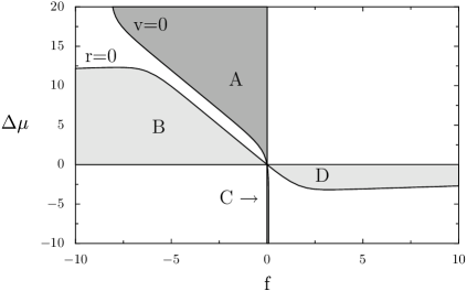
Figure 3: Four modes of operation of a molecular motor, as delimited by $\bar{v}=0$ and $r=0$ Jülicher et al. (1997). The lines are generated with parameters that we have extracted by fitting the data for kinesin in Ref. Schnitzer and Block (1997) to our model, and this fit is shown in fig. 4.

From the conditions of vanishing of the currents: $\bar{v}=0$ and $r=0$, we can construct a full operation diagram of a motor, as shown in Fig. 3 for the case of kinesin. The curves $\bar{v}=0$ and $r=0$ define implicitly $f=f_{\mbox{\scriptsize st}}(\Delta\mu)$ (the stalling force) and $\Delta\mu=\Delta\mu_{\mbox{\scriptsize st}}(f)$, respectively. The stalling force is

$$f_{\mbox{\scriptsize st}}(\Delta\mu)=\frac{1}{2}\ln\left(\frac{\left(\alpha+\omega\right)\left(\alpha^{\prime}e^{\Delta\mu}+\omega^{\prime}\right)}{\left(\alpha e^{\Delta\mu}+\omega\right)\left(\alpha^{\prime}+\omega^{\prime}\right)}\right),$$ (24)

which means that for $f=f_{\mbox{\scriptsize st}}(\Delta\mu)$, $v=0$ and $\Psi=0$, where $\Psi$ was defined in Eq. 12. At the stalling point, the mechanical variable is equilibrated but not the chemical variable. Therefore, in general, the motor consumes ATP i.e., $r\neq 0$, even if it is stalled (in fact, it is only at equilibrium, $f=\Delta\mu=0$, that both $v$ and $r$ vanish). Near stalling for $\Delta\mu\neq 0$, the motor evolves in a quasi-static manner but irreversibly. A similar phenomenon occurs in thermal ratchets Sekimoto (1997); Parrondo and Español (1996).

Likewise, the condition $\Delta\mu=\Delta\mu_{\mbox{\scriptsize st}}(f)$ means that $r=0$. The explicit form of $\Delta\mu_{\mbox{\scriptsize st}}(f)$ is

$$\Delta\mu_{\mbox{\scriptsize st}}(f)=\ln\frac{\left(\alpha e^{-\theta_{b}^{-}f}+\alpha^{\prime}e^{\theta_{b}^{+}f}\right)\left(\omega e^{\theta_{a}^{+}f}+\omega^{\prime}e^{-\theta_{a}^{-}f}\right)}{\left(\alpha e^{\theta_{a}^{+}f}+\alpha^{\prime}e^{-\theta_{a}^{-}f}\right)\left(\omega e^{-\theta_{b}^{-}f}+\omega^{\prime}e^{-\theta_{b}^{+}f}\right)}.$$ (25)

The four different regimes of operation of the motor, discussed in Refs. Jülicher et al. (1997); Lau et al. (2007) for ratchet models can be recovered here. In Region A, where $r\Delta\mu>0$ and $f\bar{v}<0$, the motor uses chemical energy of ATP to perform mechanical work. This can be understood by considering a point on the y-axis of Fig. 3 with $\Delta\mu>0$. There we expect that the motor drifts to the right with $\bar{v}>0$. Now in the presence of a small load $f<0$ on the motor, we expect that the motor is still going in the same direction although the drift is uphill and thus work is performed by the motor at a rate $\dot{W}=-f\bar{v}>0$. This holds as long as $f$ is smaller than the stalling force, which defines the other boundary of region A. Similarly, in Region B, where $r\Delta\mu<0$ and $f\bar{v}>0$, the motor produces ATP from mechanical work. In Region C, where $r\Delta\mu>0$ and $f\bar{v}<0$, the motor uses ADP to perform mechanical work. In Region D, where $r\Delta\mu<0$ and $f\bar{v}>0$, the motor produces ADP from mechanical work. It is interesting to note that the large asymmetry between regions A and C in Fig. 3 reflects the fact that kinesin is a unidirectional motor. Furthermore the regions A and B do not touch except at the origin. With kinesin operating in normal conditions in region A with $\Delta\mu\simeq 15$, the presence of a gap between regions A and B means that kinesin should not be able to switch into an ATP producing unit (region B), and indeed this has never been observed experimentally. Note that the explicit expressions for $f_{\mbox{\scriptsize st}}$ and $\Delta\mu_{\mbox{\scriptsize st}}$ obtained in this model do not depend on the energy difference $\epsilon$ between the two states, due to a cancellation of the numerator and denominator in Eqs. 21-22. Thus the diagram of operation of the motor is valid for arbitrary value of $\epsilon$.

III.3 Fit of experimental curves of velocity versus force for kinesin

We now discuss how the parameters of the model were determined using experimental data obtained for kinesin. In fig. 4 (which is also fig. 4 of Ref. Lau et al. (2007)), we have fitted velocity vs. force curves for two values of ATP concentrations, and also several curves of velocity vs. ATP concentration at different forces using the data of Ref. Schnitzer and Block (1997). We have assumed that $e^{\Delta\mu}=k_{0}\,[\mbox{ATP}]$, which is well verified at moderate or high levels of ATP. At low concentration of ATP, there is no such simple correspondence because it is no more legitimate to treat the ADP and P concentrations as constant. We think that this is probably the reason why the fit is not as good for the lowest ATP values (this concerns the first point in the curve at $F_{e}=-5.63$ pN and low ATP value in fig. 4). Nevertheless, we can fit very well the majority of the experimental points with this model and we obtained the following values for the parameters: $\epsilon=10.81$, $k_{0}=1.4\cdot 10^{5}\,\mbox{$\mu$M}^{-1}$, $\alpha=0.57\,\mbox{s}^{-1}$, $\alpha^{\prime}=1.3\cdot 10^{-6}\,\mbox{s}^{-1}$, $\omega=3.5\,\mbox{s}^{-1}$, $\omega^{\prime}=108.15\,\mbox{s}^{-1}$, $\theta^{+}_{a}=0.25$, $\theta^{-}_{a}=1.83$, $\theta^{+}_{b}=0.08$, and $\theta^{-}_{b}=-0.16$. These values are reasonable within the present accepted picture of the nano-operation of kinesin Howard (2001). Indeed, $\epsilon$ and $k_{0}^{-1}$ represent, respectively, the typical binding energy ($\sim 10\,k_{B}T$) of kinesin with microtubules and the ATP concentration at equilibrium ($\sim 10^{-5}\,\mbox{$\mu$M}$). Moreover, $\theta^{-}_{a}=1.83$ indicates that the back-steps (transitions $a\rightarrow b$) of kinesin contain most of the force sensitivity Howard (2001). Furthermore, our framework allows us to estimate a maximum stalling force of $-7\,\mbox{pN}$.

A useful quantity to consider is the distance $\ell$, which the motor walk using the hydrolysis of one ATP molecule, which is

$$\ell=\frac{\bar{v}}{r}.$$ (26)

We find for this model in agreement with Ref. Schnitzer and Block (1997) that $\ell\simeq 0.97(2d)$ in the absence of load, which corresponds to one step (8nm) per hydrolysis of one ATP molecule. Thus the coupling ratio of kinesin is indeed independent of ATP concentration and is 1:1 at negligible loads. We also find a global ATP consumption rate of $r\simeq 111\,\mbox{s}^{-1}$, in excellent agreement with known values Howard (2001). It should be remarked that the global ATP consumption rate measurements done in ATPase assays in the bulk are in agreement with the single molecule experiments, which are intrinsically very different experiments. Kinesin is well described by tightly coupled models which incorporate a single mechanically sensitive rate and this is consistent with our findings that there is only one transition (transitions $a\rightarrow b$) that has all the force sensitivity i.e., the largest load distribution factor. In principle, by changing the parameters of the model, we could characterize motors which are less tightly coupled, but there will always be some coupling because, by construction, the mechanical steps are intrinsically linked with the chemical cycle.

We have compared our fit with that carried out by Fisher et al. in Ref. Fisher and Kolomeisky (1999) where the same data was fitted, and we observe that the outcome of both fits is comparable. In this comparison, there is an issue of complexity of the model under consideration to be taken into account. This is especially important in fitting experimental data of kinetics, which is typically hard to fit because one has many parameters to fit in an expression which is a sum of exponential functions. The model of Ref. Fisher and Kolomeisky (1999) is of higher complexity because it involves 4 states instead of 2 states for our model, thus we might be tempted to say that our model does better in fitting the same data with less complexity. We believe that this is true when considering the data for the velocity only, but if we were to include also the data for the diffusion coefficient (which is related to the randomness parameter defined in Ref. Schnitzer and Block (1997)), we agree with Ref. Fisher and Kolomeisky (1999) that a model with 4 states would then do better than a model with only 2 states.

III.4 Thermodynamic Efficiency

Another important quantity that characterizes the working of a motor is its efficiency Sekimoto (1997); Jülicher et al. (1997). In region A, it is defined as the ratio of the work performed to the chemical energy:

$$\eta=-\frac{f\bar{v}}{r\Delta\mu}=-\frac{f\ell}{\Delta\mu}.$$ (27)

By definition, $\eta$ vanishes at $f=0$ and at the stalling force $f_{\mbox{\scriptsize st}}(\Delta\mu)$. Therefore, it has a local maximum $\eta_{\mbox{\scriptsize m}}(\Delta\mu)$ for some $f_{\mbox{\scriptsize m}}(\Delta\mu)$ between $f_{\mbox{\scriptsize st}}<f_{\mbox{\scriptsize m}}<0$. Near equilibrium, $\eta_{\mbox{\scriptsize m}}(\Delta\mu)$ has a constant value, $\eta_{\mbox{\scriptsize m}}^{\mbox{\scriptsize eq}}$, along a straight line $f_{\mbox{\scriptsize m}}(\Delta\mu)\propto\Delta\mu$ inside region A Jülicher et al. (1997). However, far from equilibrium, the picture is drastically different. We find that (i) $f_{\mbox{\scriptsize m}}(\Delta\mu)$ is no longer a straight line, (ii) $\eta_{\mbox{\scriptsize m}}-\eta_{\mbox{\scriptsize m}}^{\mbox{\scriptsize eq}}\propto\Delta\mu$ for small $\Delta\mu$, and (iii) $\eta_{\mbox{\scriptsize m}}\sim 1/\Delta\mu$ for large $\Delta\mu$. Therefore, $\eta_{\mbox{\scriptsize m}}$ must have an absolute maximum at some $\Delta\mu>1$. One can also consider the curves of equal value of the efficiency within region A. In the particular case of the linear regime close to equilibrium, these curves are straight lines going through the origin Jülicher et al. (1997), but in general far from equilibrium these curves are not straight lines as can be seen in Fig. 5, and the maximum efficiency is reached at a point within region A.

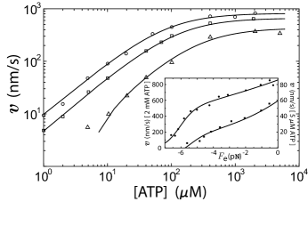
Figure 4: Kinesin velocity vs. ATP concentration under an external force Lau et al. (2007). The solid curves are the fits of our model to data from Ref. Schnitzer and Block (1997). From the top down, the plots are for $F_{e}=-1.05,-3.59$, and $-5.63\,\mbox{pN}$, respectively. Inset: Kinesin velocity vs. force under a fixed ATP concentration. The solid curves are fits to the data of Ref. Schnitzer and Block (1997). From the top down, the plots are for $[\mbox{ATP}]=2\,\mbox{mM}$ and $5\,\mbox{$\mu$M}$. From this fit, we obtained the following parameters for our model : $\epsilon=10.81$, $k_{0}=1.4\cdot 10^{5}\,\mbox{$\mu$M}^{-1}$, $\alpha=0.57\,\mbox{s}^{-1}$, $\alpha^{\prime}=1.3\cdot 10^{-6}\,\mbox{s}^{-1}$, $\omega=3.5\,\mbox{s}^{-1}$, $\omega^{\prime}=108.15\,\mbox{s}^{-1}$, $\theta^{+}_{a}=0.25$, $\theta^{-}_{a}=1.83$, $\theta^{+}_{b}=0.08$, and $\theta^{-}_{b}=-0.16$.

Figure 5: Curves of equal efficiency $\eta$ within region A (which is delimited by the solid line and by the $y$ axis). The parameters are those used in fig. 3 and obtained from the fit of fig. 4. From the outside to the inside the curves correspond to $\eta=0.2$, $\eta=0.3$, $\eta=0.4$, $\eta=0.5$ and $\eta=0.58$. The absolute maximum efficiency for these parameters is about 59% and is located at $\Delta\mu\simeq 14$ and $f\simeq-4.9$.

Note that $\eta_{\mbox{\scriptsize m}}$ is substantially larger than $\eta_{\mbox{\scriptsize m}}^{\mbox{\scriptsize eq}}$. For instance with the parameters used in fig. 5, the maximum efficiency is around 0.59 while $\eta_{\mbox{\scriptsize m}}^{\mbox{\scriptsize eq}}\simeq 0.03$ (see also Fig. 3b of Ref. Lau et al. (2007) which contains a plot of $\eta_{\mbox{\scriptsize m}}$ as a function of $\Delta\mu$ under the same conditions). Hence, this motor achieves a higher efficiency in the far-from-equilibrium regime as was also found in other studies of molecular motors using continuous ratchet models (see e.g., Ref. Parmeggiani et al. (1999)). Under typical physiological conditions ($\Delta\widetilde{\mu}\sim 10-25\,\mbox{$k_{B}T$}$), kinesin operates at an efficiency in the range of $40-60\%$, in agreement with experiments Howard (2001). It is interesting to note that kinesins operate most efficiently in an energy scale corresponding to the energy available from ATP hydrolysis.

IV Finite time and long time fluctuation theorem

IV.1 Long time FT

We note that the rates of Eq. 8 satisfy the following generalized detailed balance conditions:

$$\overrightarrow{\omega_{b}}^{-l}P_{b}^{\mbox{\scriptsize eq}} = \overleftarrow{\omega_{a}}^{l}P_{a}^{\mbox{\scriptsize eq}}\,e^{+(\,\theta^{-}_{a}+\theta^{+}_{b}\,)f-\Delta\mu\,l},$$ (28)

$$\overleftarrow{\omega_{b}}^{-l}\,P_{b}^{\mbox{\scriptsize eq}} = \overrightarrow{\omega_{a}}^{l}P_{a}^{\mbox{\scriptsize eq}}\,e^{-(\,\theta^{+}_{a}+\theta^{-}_{b}\,)f-\Delta\mu\,l},$$ (29)

for $l=0,1$. Here, $P_{a}^{\mbox{\scriptsize eq}}=1/(1+e^{-\epsilon})$ and $P_{b}^{\mbox{\scriptsize eq}}=e^{-\epsilon}/(1+e^{-\epsilon})$ are the equilibrium probabilities corresponding to $f=0$ and $\Delta\mu=0$. We note that these relations, Eq. 28 and Eq. 29, while valid arbitrarily far from equilibrium, still refer to the equilibrium state via the probabilities $P_{i}^{eq}$. Using the definition of the equilibrium probabilities, one can in fact rewrite Eqs. 28-29 as

$$\ln\frac{\overrightarrow{\omega_{b}}^{-l}}{\overleftarrow{\omega_{a}}^{l}} = \epsilon+\left(\theta^{-}_{a}+\theta^{+}_{b}\,\right)f-\Delta\mu\,l,$$ (30)

$$\ln\frac{\overleftarrow{\omega_{b}}^{-l^{\prime}}}{\overrightarrow{\omega_{a}}^{l^{\prime}}} = \epsilon-\left(\theta^{+}_{a}+\theta^{-}_{b}\,\right)f-\Delta\mu\,l^{\prime},$$ (31)

for $l,l^{\prime}=0,1$. Note that these relations are analogous to the De Donder relation of Eq. 9 and to the transition state theory equations of Eqs. 4-5. Moreover, by combining these two equations, using the constraint that the sum of the load distribution factors is two and then multiplying the result by $k_{B}T$, one obtains

$$k_{B}T\ln\frac{\overrightarrow{\omega_{b}}^{-l}\overrightarrow{\omega_{a}}^{l^{\prime}}}{\overleftarrow{\omega_{a}}^{l}\overleftarrow{\omega_{b}}^{-l^{\prime}}}=F_{e}(2d)-\Delta\tilde{\mu}\left(l-l^{\prime}\right),$$ (32)

which has the form of the steady state balance condition discussed in Refs liepelt; seifert_entropy. As pointed out in these references, by identifying the left hand side of Eq. 32 with the heat delivered to the medium, i.e. with the change of entropy of the medium, the right hand side of Eq. 32 can be interpreted as the sum of the mechanical work $F_{e}(2d)$ and the chemical work $-\Delta\tilde{\mu}\left(l-l^{\prime}\right)$ on that particular set of cyclic transitions $(l,l^{\prime})$. In that sense, Eqs. 30-32 can be understood as formulations of the first law at the level of elementary transitions. It is interesting to see that these steady state balance relations also lead to a FT as we now show below.

Using Eqs. (28) and (29), it can be shown that ${\cal M}$ and ${\cal M}^{{\dagger}}$, the adjoint of ${\cal M}$, are related by a similarity transformation:

$${\cal M}^{{\dagger}}[\,f-\lambda,\Delta\mu-\gamma]={\cal Q}\,{\cal M}[\lambda,\gamma]\,{\cal Q}^{-1},$$ (33)

where ${\cal Q}$ is the following diagonal matrix:

$${\cal Q}=\left[\begin{array}[]{cc}P_{b}^{eq}e^{(\theta_{a}^{+}+\theta_{b}^{-})f/2}&0\\ 0&P_{a}^{eq}e^{(\theta_{a}^{-}+\theta_{b}^{+})f/2}\\ \end{array}\right].$$ (36)

This similarity relation implies that ${\cal M}[\lambda,\gamma]$ and ${\cal M}^{{\dagger}}[\,f-\lambda,\Delta\mu-\gamma]$ have the same spectra of eigenvalues and therefore

$$\vartheta[\lambda,\gamma]=\vartheta[\,f-\lambda,\Delta\mu-\gamma],$$ (37)

which is one form of FT. Since this relation holds at long times irrespective of the initial state, it is a Gallavotti-Cohen relation Evans et al. (1993). Such a symmetry is illustrated graphically on Fig. 6 for a simplified case where the chemical variable is absent.

Figure 6: Graphical illustration of the symmetry of the long-time Fluctuation Theorem (for simplicity a model without chemical variable has been used). The largest eigenvalue $\vartheta$ is shown as function of $\xi=\lambda/f$ for different values of the normalized force $f$. The symmetry of the long time Fluctuation Theorem corresponds to the symmetry of this curve with respect to $\xi=1/2$.

IV.2 Implications of FT in the linear regime

Here, we discuss the implications of FT in the linear regime, which leads to the Einstein and Onsager relations near equilibrium. Differentiating Eq. 37 with respect to $\lambda$ and $\gamma$, we obtain:

$$\bar{v}=-\frac{\partial\vartheta}{\partial\lambda}[\,0,0] = \frac{\partial\vartheta}{\partial\lambda}[\,f,\Delta\mu],$$ (38)

$$r=-\frac{\partial\vartheta}{\partial\gamma}[\,0,0] = \frac{\partial\vartheta}{\partial\gamma}[\,f,\Delta\mu].$$ (39)

The response and fluctuations of a motor are quantified, respectively, by a response matrix $\lambda_{ij}$ and by the diffusion matrix $D_{ij}$ defined in Eq. 23. The physical meanings of $\lambda_{ij}$ are: $\lambda_{11}\equiv\partial\bar{v}/\partial f$ is the mobility, $\lambda_{22}\equiv\partial r/\partial\Delta\mu$ is the chemical admittance, and $\lambda_{12}\equiv\partial\bar{v}/\partial\Delta\mu$ and $\lambda_{21}\equiv\partial r/\partial f$ are the Onsager coefficients that quantify the mechanochemical couplings of the motor. Near equilibrium, where $f$ and $\Delta\mu$ are small, a Taylor expansion of the r.h.s. of Eq. 38 and Eq. 39 with respect to $f$ and $\Delta\mu$ leads to

$$\left.\frac{\partial\vartheta}{\partial\lambda}\right|_{\,f,\Delta\mu} \simeq \left.\frac{\partial\vartheta}{\partial\lambda}\right|_{0,0}+f\left.\frac{\partial^{2}\vartheta}{\partial^{2}\lambda}\right|_{0,0}+\Delta\mu\left.\frac{\partial^{2}\vartheta}{\partial\lambda\partial\gamma}\right|_{0,0},$$ (40)

$$\left.\frac{\partial\vartheta}{\partial\gamma}\right|_{\,f,\Delta\mu} \simeq \left.\frac{\partial\vartheta}{\partial\gamma}\right|_{0,0}+f\left.\frac{\partial^{2}\vartheta}{\partial\gamma\partial\lambda}\right|_{0,0}+\Delta\mu\left.\frac{\partial^{2}\vartheta}{\partial^{2}\gamma}\right|_{0,0}.$$ (41)

Using the definitions of $\bar{v}$ and $r$ from Eqs. 38-39, one obtains directly

$$\bar{v} = \lambda_{11}^{0}\,f+\lambda_{12}^{0}\,\Delta\mu,$$ (42)

$$r = \lambda_{21}^{0}\,f+\lambda_{22}^{0}\,\Delta\mu,$$

with $\lambda_{ij}^{0}=\partial_{z_{i}}\partial_{z_{j}}\vartheta[\,0,0]/2\equiv D_{ij}$, which are the Einstein relations, and $\lambda_{12}^{0}\equiv\partial_{\gamma}\partial_{\lambda}\vartheta[\,0,0]/2=\partial_{\lambda}\partial_{\gamma}\vartheta[\,0,0]/2\equiv\lambda_{21}^{0}$, which is the Onsager relation. Thus, FT describes the response and fluctuations near equilibrium Gallavotti (1996); Gaspard and Gerritsma (2007).

It is interesting to investigate how Einstein or Onsager relations are broken in non-equilibrium situations. The ”violations” of Einstein and Onsager relations when linear response theory is used in the vicinity of a non-equilibrium state rather than near an equilibrium state were studied in Ref. Lau et al. (2007). There, we quantified the violations of Einstein and Onsager relations, respectively, by four temperature-like parameters, $T_{ij}$, and by the difference of the mechanochemical coupling coefficients, $\Delta\lambda$. Of course, these effective temperatures are not thermodynamic temperatures: they are merely one of the ways to quantify deviations from Einstein relations; similarly our definition of $\Delta\lambda$ is just one of the possible ways to study the ”violations” of Onsager relations: strictly speaking there are no real violations since Einstein and Onsager relations apply only to systems at equilibrium. We have shown in Lau et al. (2007) some of the possible behaviors of $T_{ij}$ and $\Delta\lambda$ for a kinesin motor using the parameters of the fit discussed above: in particular, we found that for kinesin the maximum value of $\Delta\lambda$ is $\Delta\lambda\sim 45\,\mbox{pN}^{-1}\mbox{s}^{-1}$, and that at large $\Delta\mu$, $\Delta\lambda\sim-10\,\mbox{pN}^{-1}\mbox{s}^{-1}$. We also found that (i) one of the Einstein relations holds near stalling (a point which we justify more precisely in the next section in Eq. 70), (ii) the degree by which the Onsager symmetry is broken ($\Delta\lambda\neq 0$) is largely determined by the underlying asymmetry of the substrate, (iii) only two “effective” temperatures characterize the fluctuations of tightly coupled motors, (iv) kinesin’s maximum efficiency and the maximum violation of Onsager symmetry occur roughly at the same energy scale, corresponding to that of ATP hydrolysis ($\sim 20\,k_{B}T$) Lau et al. (2007). Experimental and theoretical violations of the Fluctuation-Dissipation relation have been observed and studied in many active biological systems Martin et al. (2001); Manneville et al. (2001); Kruse et al. (2003); Mizuno et al. (2007); Lau et al. (2003), but to our knowledge no experiments testing the Fluctuation-Dissipation or the Onsager relations have been carried out at the single motor level.

IV.3 Finite time FT

Figure 7: Graphical illustration of the symmetry of the finite-time Fluctuation Theorem for a simplified model without chemical variable. The left hand side of Eq. IV.3 is shown as function of $\xi=\lambda/f$ for different times (arbitrary units). The symmetry of the finite time Fluctuation Theorem amounts to the symmetry of this curve with respect to $\xi=1/2$.

The similarity transformation (33) implies that all the eigenvalues of ${\cal M}[\lambda,\gamma]$ and ${\cal M}^{{\dagger}}[\,f-\lambda,\Delta\mu-\gamma]$ are identical, not just the largest one. This more general property allows us to prove a transient FT, because the dynamics of the model at finite time involves all the eigenvalues of ${\cal M}$ and not just the largest one. The price to pay to have a FT relation valid at finite time is that the initial state can no more be arbitrary. We show here that the relation still holds, in the particular case when the initial state is prepared to be in an equilibrium state (which corresponds to the condition $f=\Delta\mu=0$) and when, in addition, a specific condition on the load distribution factors is obeyed. To see how this comes about in this model, we assume that the motor at time $t=0$ is at the origin $n(0)=y(0)=0$ in an equilibrium state, and we calculate the values of the position $n(t)$ and of the chemical variable $y(t)$ at time $t$. We denote the initial state by the vector

$$|F_{0}\rangle=|F(t=0)\rangle=\left(\begin{array}[]{c}P_{a}^{eq}\\ P_{b}^{eq}\\ \end{array}\right).$$ (45)

With $\langle 0|=(1,1)$, the initial state vector is normalized since $\langle 0|F_{0}\rangle=1$. Let us introduce ${\cal U}(\lambda,\gamma,t)=e^{{\cal M}[\lambda,\gamma]t}$, the evolution operator for the generating functions $F_{i}$. By taking the exponential of Eq. 33, one finds that this operator also obeys an FT relation

$${\cal U}^{{\dagger}}[\,f-\lambda,\Delta\mu-\gamma,t]={\cal Q}\,{\cal U}[\lambda,\gamma,t]\,{\cal Q}^{-1}.$$ (46)

We calculate the following average, similar to Eq. 17,

$$\langle e^{-(f-\lambda)n(t)-(\Delta\mu-\gamma)y(t)}\rangle = \langle 0|{\cal U}(f-\lambda,\Delta\mu-\gamma,t)|F_{0}\rangle,$$

$$= \langle F_{0}|{\cal U}^{\dagger}(f-\lambda,\Delta\mu-\gamma,t)|0\rangle,$$

$$= \langle F_{0}|{\cal Q}{\cal U}(\lambda,\gamma,t){\cal Q}^{-1}|0\rangle,$$

$$= \langle 0|{\cal U}(f,\gamma,t)|F_{0}\rangle,$$

$$= \langle e^{-\lambda n(t)-\gamma y(t)}\rangle.$$

We have used Eq. 46 to derive the third equality, and the final equation requires the condition: $\langle F_{0}|{\cal Q}=\langle 0|$, which is equivalent to ${\cal Q}^{-1}|0\rangle=|F_{0}\rangle$ since ${\cal Q}$ is diagonal. Using Eq. 36, we find that this relation holds if the initial state is in equilibrium and if the following condition holds

$$\theta_{a}^{-}+\theta_{b}^{+}=\theta_{a}^{+}+\theta_{b}^{-}.$$ (48)

Equation IV.3 is analogous to the Evans transient time Fluctuation Theorem Evans and Searles (2002) and to the Crooks relation Crooks (2000). An important point here is that the initial state must be an equilibrium state while the final state at time $t$ does not have to be (and in general is not) an equilibrium state. Crooks relation can be derived using a path representation of the ratio of forward to backward probabilities according to a specific protocol, assuming a Markov process and using a generalized detailed balance relation between successive states. In our case, the equivalent of the generalized ”local” detailed balance condition needed for the proof is Eq. 46. The symmetry of the transient Fluctuation Theorem is illustrated graphically in Fig. 7 for a simplified case where the chemical variable is absent (or integrated out).

V Fluctuation Theorem for the large deviation function

V.1 Explicit calculation of the large deviation function of the current

Here, we again take advantage of our knowledge of the function $\vartheta$, which contains all the information about the long time dynamical properties of the model, to obtain an explicit expression for the large deviation function of the current. To simplify the presentation, we consider the simplified description, given in Eq. 10, in which the chemical variable $y$ is not taken into account. In this case, the generating function is defined by $F_{i}(\lambda,t)\equiv\sum_{y}\sum_{n}e^{-\lambda n}P_{i}(n,y,t),$ and the matrix ${\cal M}[\lambda]$ becomes

$${\cal M}[\lambda]=\left[\begin{array}[]{cc}-\overrightarrow{\omega_{a}}-\overleftarrow{\omega_{a}}&e^{\lambda}\,\overleftarrow{\omega_{b}}+e^{-\lambda}\,\overrightarrow{\omega_{b}}\\ e^{\lambda}\,\overleftarrow{\omega_{a}}+e^{-\lambda}\,\overrightarrow{\omega_{a}}&-\overleftarrow{\omega_{b}}-\overrightarrow{\omega_{b}}\\ \end{array}\right].$$ (51)

By definition, $\vartheta$ is the largest eigenvalue of ${\cal M}(\lambda)$, so similarly to Eq. III.1 we have

$$\vartheta(\lambda)= \frac{1}{2} \{-\omega_{a}-\omega_{b}+[(\omega_{a}-\omega_{b})^{2}$$

$$+ 4(\overleftarrow{\omega}_{b}e^{\lambda}+\overrightarrow{\omega}_{b}e^{-\lambda})(\overleftarrow{\omega}_{a}e^{\lambda}+\overrightarrow{\omega}_{a}e^{-\lambda})]^{1/2}\},$$

with the notations $\omega_{a}=\overrightarrow{\omega}_{a}+\overleftarrow{\omega}_{a}$ and $\omega_{b}=\overrightarrow{\omega}_{b}+\overleftarrow{\omega}_{b}$.

We have already seen that $\vartheta(\lambda)$ has the property that $<e^{-\lambda n}>\sim e^{\vartheta(\lambda)t}$ for large $t$. On the other hand, the large deviation function $G(v)$ is defined for large time $t$ by

$$\mathcal{P}(\frac{n}{t}=v)\sim e^{-G(v)t},$$ (54)

in terms of $\mathcal{P}(n/t=v)$ the probability to observe a current $v$ after the motor has gone a distance $n$ from the origin in a time $t$. The relation between $\vartheta(\lambda)$ and $G(v)$ is

$$<e^{-\lambda n}> = \int e^{-\lambda n}dn\mathcal{P}(n),$$ (55)

$$= \int tdv\mathcal{P}(\frac{n}{t}=v)e^{-\lambda vt},$$ (56)

$$\sim \int dve^{\left(-G(v)-\lambda v\right)t}.$$ (57)

Using the saddle point method, we find that $\vartheta(\lambda)=\max_{v}(-G(v)-\lambda v)$ and thus $\vartheta(\lambda)$ and $G(v)$ are Legendre transform of each other. We have also $-G(v)=\max(\vartheta(\lambda)+\lambda v)$, which can be written in parametric form

$$\frac{\partial\vartheta}{\partial\lambda}[\lambda=\lambda^{*}]+v = 0,.$$ (58)

$$\vartheta(\lambda^{*})+\lambda^{*}v = -G(v).$$ (59)

Using Eqs. V.1-59, we find the following expressions for $G(v)$ (see Appendix A for details of the derivation): for $v>0$

$$G(v)=\frac{\omega_{a}+\omega_{b}}{2}+\frac{\sqrt{\Omega}}{2v}\left(Y^{-}(v)-\frac{1}{Y^{-}(v)}\right)-v\lambda^{-}(v),$$ (60)

and for $v<0$,

$$G(v)=\frac{\omega_{a}+\omega_{b}}{2}+\frac{\sqrt{\Omega}}{2v}\left(Y^{+}(v)-\frac{1}{Y^{+}(v)}\right)-v\lambda^{+}(v),$$ (61)

where

$$Y^{\pm}(v) = \frac{1}{2}\left(Z(v)\pm\sqrt{Z(v)^{2}-4}\right),$$

$$\lambda^{\pm}(v) = -\frac{\Psi}{2}+\frac{1}{2}\ln\left(\frac{Z(v)\pm\sqrt{Z(v)^{2}-4}}{2}\right),$$ (62)

and

$$Z(v)=\frac{v^{2}}{\sqrt{\Omega}}+\left(\frac{v^{4}}{\Omega}+4+\frac{v^{2}\Sigma^{2}}{\Omega}\right)^{1/2},$$ (63)

with the following parameters

$$\Omega = 4\overrightarrow{\omega}_{a}\overrightarrow{\omega}_{b}\overleftarrow{\omega}_{a}\overleftarrow{\omega}_{b},$$ (64)

$$\Sigma^{2} = \left(\omega_{a}+\omega_{b}\right)^{2}-4\left(\overleftarrow{\omega}_{a}\overleftarrow{\omega}_{b}+\overrightarrow{\omega}_{a}\overrightarrow{\omega}_{b}\right),$$ (65)

and $\Psi$ is the effective potential defined in Eq. 11.

Figure 8: Large deviation function $G(v)$, the solid line is the exact expression using Eqs. 60-61 and the points are the numerical evaluation of the Legendre transform using Eq. 59. For the values of the rates used here, the average velocity, as given by Eq. 21, is $\bar{v}\simeq 80$: thus, the system is far from equilibrium. Note that $G(v)$ is minimum at $\bar{v}$ and that $G(\bar{v})=0$.

As shown in fig. 8, the function $G(v)$ has a single minimum at the average velocity $v=\bar{v}$, which was defined in Eq. 21, and at this point $G(v=\bar{v})=0$, which can be deduced from Eq. 59. Remarkably, although $G(v)$ is a complicated non-linear function of $v$, the difference $G(v)-G(-v)$ is a simple linear function of $v$ as required by the Fluctuation Theorem. Using the expressions (59) and (60), it is straightforward to verify that

$$G(v)-G(-v)=\Psi v,$$ (66)

which in turns implies that the ratio of the probabilities to observe $v$ or $-v$ for large $t$ must obey:

$$\frac{\mathcal{P}(\frac{n}{t}=v)}{\mathcal{P}(\frac{n}{t}=-v)}=e^{-\Psi vt}.$$ (67)

From Eq. 66, and the fact that $G(v)$ and $\vartheta(\lambda)$ are related by a Legendre transform, we obtain a third formulation of the Fluctuation Theorem:

$$\vartheta(\lambda)=\vartheta(-\Psi-\lambda).$$ (68)

Near equilibrium, the large deviation function is well approximated by a half parabola when both $v$ when $\bar{v}$ are either positive or negative. For $\bar{v}>0$, this part of the large deviation function becomes flatter and flatter, when going away from equilibrium (i.e., for increasing entropy production). As a result, the remaining part of the large deviation function for $v<0$ must be linear $G(v<0)\simeq-\Psi v$, so that Eq. 66 is obeyed. This linear part for $v<0$ and the half parabola for $v>0$ can be seen in fig. 8.

It is interesting to note the central role played by the quantity $\Psi$ defined initially as an effective potential, and which now enters the three formulations of the Fluctuation Theorem in Eqs. 66-68. Note that these equations were obtained for arbitrary forms of the rates $\overrightarrow{\omega}_{a},\overrightarrow{\omega}_{b},\overleftarrow{\omega}_{a}$ and $\overleftarrow{\omega}_{b}$. If we make a specific choice for these rates as in Eq. 8, with no chemistry i.e., for $\Delta\mu=0$, we recover $\Psi=-f$, and then Eq. 68 reduces to $\vartheta(f-\lambda)=\vartheta(\lambda)$, which is indeed compatible with Eq. 37 when there is no chemical variable and no dependance on the rates on chemistry. If the rates are those of Eq. 8 for $\Delta\mu\neq 0$, we obtain using Eq. 12, the expression

$$\frac{\mathcal{P}(\frac{n}{t}=v)}{\mathcal{P}(\frac{n}{t}=-v)}=e^{(f-f_{st}(\Delta\mu))vt},\,\,\,\,(\rm{for}\,t\rightarrow\infty)$$ (69)

with the stalling force defined in Eq. 24, and related to $\Psi$ by $\Psi=-f+f_{st}(\Delta\mu)$.

Note that an Einstein relation can be obtained near stalling, by performing a Taylor expansion of the r.h.s of Eq. 68 with respect to $-\Psi$, in way similar to what was done in Eqs. 40-41 for the derivation of the Einstein and Onsager relations. This procedure means that for $f\simeq f_{st}(\Delta\mu)$,

$$\bar{v}\simeq\frac{1}{2}\left(f-f_{st}(\Delta\mu)\right)\left.\frac{\partial^{2}\vartheta}{\partial^{2}\lambda}\right|_{0},$$ (70)

which shows that near the stalling force, the Einstein relation holds in this description where the chemical variable is absent Lau et al. (2007).

V.2 Discussion

Note that Eq. 69 puts a constraint on the ratio of the probabilities of observing a velocity $v$ to the probability of observing a velocity $-v$. These velocities should be estimated from the ratio $n/t$ based on an observation of the motor running a distance $n$ (or a distance $-n$), after a time $t$. This relation has been proven here in the limit of long time $t$, but we expect that such a relation will also hold at finite time $t$ under some conditions, as suggested by our derivation of the transient FT of Eq. IV.3. Such a relation at finite time was also investigated in Ref. Gaspard and Gerritsma (2007).

Single molecule experiments on kinesin in which backward steps were studied were performed in Refs. Nishiyama et al. (2002); Carter and Cross (2005). In particular it was shown in these references that ATP binding was necessary for backward steps, and that the ratio of the overall probability of making one forward step (whatever the time) to the overall probability of making one backward step (whatever the time) is an exponential function of the load, which approaches one near the stalling force. It is important to point out that this ratio which was measured experimentally is not the same quantity as the left hand side of Eq. 69 although both quantities should be related. In view of this, Eq. 69 should be considered as a prediction for the behavior of single motors like kinesin, which to our knowledge has not yet been tested experimentally. This suggests that it would be very interesting to probe Eq. 69 experimentally, by trying to compute directly the distributions $\mathcal{P}(\frac{n}{t}=\pm v)$ for various times. At the same time, it would be also useful to study more extensively the behavior of motors of various types near stalling as function of the ATP concentration. No notable difference could be measured in the stalling force at an ATP concentration $1m$M or $10\mu$M in the experiments of Carter and Cross (2005) on kinesin, although in principle according to general grounds Lipowsky (2000); liepelt one should expect that the behavior of motors near stalling (and in particular the stalling force of the motor itself) should depend on the ATP concentration and more generally on the details of the chemical cycle of ATP hydrolysis.

V.3 Other forms of FT relations

We have seen that the form of the FT relation depends on the state variables of the system, or in other words, it depends on the level of coarse-graining of the description. We consider in this paper the following levels of description:

• (I): The mechanical displacement $n$ is the only state variable.

• (II): The chemical variable $y$ is the only state variable.

• (III): Both variables $n$ and $y$ are taken into account.

For case (I), the dynamics is described by the simplified master equation, Eq. 10 and Eqs. (66-68) are the appropriate forms of FT.

For case (II), we find that FT can be written in the following forms (we shall omit the large deviation function form of FT for cases (II) and (III)):

$$\frac{\mathcal{P}(\frac{y}{t}=r)}{\mathcal{P}(\frac{y}{t}=-r)}=e^{-\chi rt},$$ (71)

which also holds generally for $t\rightarrow\infty$ and

$$\vartheta(\gamma)=\vartheta(-\chi-\gamma).$$ (72)

In the above two equations, $-\chi$ can be interpreted as the affinity De Donder (1927) associated with a chemical cycle (see the representation of the chemical cycle in fig. 2, and next section for a discussion on the notion of affinity). We find that $\chi$ is given by

$$\chi=\ln\left(\frac{\omega_{b}^{-1}\omega_{a}^{0}}{\omega_{a}^{1}\omega_{b}^{0}}\right),$$ (73)

where $\omega_{a}^{l}=\overrightarrow{\omega}_{a}^{l}+\overleftarrow{\omega}_{a}^{l}$ and $\omega_{b}^{l}=\overrightarrow{\omega}_{b}^{l}+\overleftarrow{\omega}_{b}^{l}$ for $l=-1,0$ or $1$. The physical interpretation of $\chi$ can be clarified by using a method similar to Kafri et al. (2004): after integrating out the position variable $n$ from Eq. 1, and decimating over the odd or even sites, one can derive an effective evolution equation for the occupation probabilities of the remaining sites. In this equation, $\chi$ plays the role of a effective potential for the chemical variable. When the rates of Eq. 8 are used, we find that this quantity is given by

$$\chi=-\Delta\mu+\Delta\mu_{st}(f)\,.$$ (74)

As expected, the conditions for which $\chi$ vanishes are the same as those for which the chemical current $r$, given in Eq. 22, vanishes.

For case (III), the FT can be written as follows

$$\frac{\mathcal{P}(\frac{n}{t}=v,\frac{y}{t}=r)}{\mathcal{P}(\frac{n}{t}=-v,\frac{y}{t}=-r)}=e^{-(\tilde{\Psi}v+\tilde{\chi}r)t},$$ (75)

for $t\rightarrow\infty$ and

$$\vartheta(\lambda,\gamma)=\vartheta(-\tilde{\Psi}-\lambda,-\tilde{\chi}-\gamma).$$ (76)

Here, the affinities associated with the mechanical and chemical variables are given, respectively, by $-\tilde{\Psi}$ and $-\tilde{\chi}$. Note that these quantities are in general not the same as the ones calculated above in cases (I) and (II) (i.e., $\tilde{\Psi}\neq\Psi$ and $\tilde{\chi}\neq\chi$). When the rates of Eq. 8 are used, $\tilde{\Psi}=-f$ and $\tilde{\chi}=-\Delta\mu$, so that Eq. 37 is recovered from Eq. 76.

VI Fluctuation Theorem and Entropy Production

In this section, we discuss the connections between the Fluctuation Theorem described in the last section and the entropy production Lebowitz and Spohn (1999). In particular, we show by an explicit calculation, that the parameters $\Psi$, $\chi$, $f$ and $\Delta\mu$ that appear in the symmetry relations Eqs. 66-69 are identical to the affinities associated with the various macroscopic currents (mechanical and chemical) flowing in the system Gaspard and Gerritsma (2007). Affinities, introduced a long time ago in chemical thermodynamics De Donder (1927), represent intrinsic quantities that depend only on the microscopic transition rates of the system. Thus, the fact that these quantities also appear in the Fluctuations Theorems, valid far from equilibrium, shows a remarkable connection between classical thermodynamics and non-equilibrium statistical mechanics.

We shall first discuss the simplified model, in which the chemical variable $y$ is not taken into account in the description as a state variable (case (I)). The mechanical entropy $S_{\rm M}(t)$ then only contains contribution from the disorder in the distribution of the mechanical variable $n$ and is defined as

$$S_{\rm M}(t)=-\sum_{i=a,b}\sum_{n}P_{i}(n,t)\ln P_{i}(n,t)$$ (77)

in units where $k_{B}=1$. Using the master equation, Eq. 10, one can calculate the variation of $S_{M}(t)$ with time:

$$\frac{dS_{\rm M}}{dt}={\hskip 170.71652pt}$$ (78)

$$\sum_{i\neq j}\sum_{n}\left(\overrightarrow{\omega}_{i}P_{i}(n,t)-\overleftarrow{\omega}_{j}P_{j}(n+1,t)\right)\ln\frac{P_{i}(n,t)}{P_{j}(n+1,t)}\,,$$

where $i,j$ take the two possible values $a$ and $b$ but are different from each other. By transforming the last term in this equation as follows

$$\ln\frac{P_{i}(n,t)}{P_{j}(n+1,t)}=\ln\frac{\overrightarrow{\omega}_{i}P_{i}(n,t))}{\overleftarrow{\omega}_{j}P_{j}(n+1,t)}-\ln\frac{\overrightarrow{\omega}_{i}}{\overleftarrow{\omega}_{j}}\,,$$

the time derivative of the entropy can be rewritten as the difference of an entropy production (which is always positive) and an entropy flux. Since we are interested in a stationary state where $dS/dt=0$, both contributions must be equal. From such a calculation, one finds that the entropy production and the entropy flux in the long time limit are given by

$$\Pi_{\rm M}=\frac{\overrightarrow{\omega}_{a}\overrightarrow{\omega}_{b}-\overleftarrow{\omega}_{a}\overleftarrow{\omega}_{b}}{\overrightarrow{\omega}_{a}+\overrightarrow{\omega}_{b}+\overleftarrow{\omega}_{a}+\overleftarrow{\omega}_{b}}\ln\left(\frac{\overrightarrow{\omega}_{a}\overrightarrow{\omega}_{b}}{\overleftarrow{\omega}_{a}\overleftarrow{\omega}_{b}}\right)=-\Psi\bar{v},$$ (79)

where $\Psi$ is the effective potential defined in Eq. 11, and $\bar{v}$ is defined in Eq. 21. According to the general definition Gaspard and Gerritsma (2007), we deduce from Eq. 79 that the mechanical affinity of the displacement variable is $-\Psi$.

It is interesting to recall that this result can also be derived in a different way : in Lebowitz and Spohn (1999), it was proven that the entropy flux can be calculated by using a fluctuating quantity $W(t)$, called the action functional, which can be seen as a local measure of the lack of detailed balance on a given path at time $t$. The matrix ${\cal N}(\nu)$ that describes the evolution of the generating function of $\langle\exp(-\nu W(t))\rangle$ is given by

$${\cal N}=\left[\begin{array}[]{cc}-\overrightarrow{\omega_{a}}-\overleftarrow{\omega_{a}}&\,\overleftarrow{\omega_{a}}^{(1-\nu)}\overrightarrow{\omega_{b}}^{\nu}+\overleftarrow{\omega_{b}}^{\nu}\overrightarrow{\omega_{a}}^{(1-\nu)}\\ \overleftarrow{\omega_{b}}^{(1-\nu)}\overrightarrow{\omega_{a}}^{\nu}+\overleftarrow{\omega_{a}}^{\nu}\overrightarrow{\omega_{b}}^{(1-\nu)}&-\overleftarrow{\omega_{b}}-\overrightarrow{\omega_{b}}\\ \end{array}\right].$$

This matrix is obtained by deforming the original Markov matrix by a parameter $\nu$. We emphasize that this deformation is not the same as that used in Eq. 51 to calculate the large deviation of the currents. The time derivative of $W(t)$ is precisely the entropy flux. Therefore, we have, in agreement with Eq. 79,

$$\Pi_{\rm M}=-\frac{\partial q}{\partial\nu}(0)=-\bar{v}\Psi,$$ (83)

where $q(\nu)$ is the largest eigenvalue of ${\cal N}(\nu)$. Since the matrix ${\cal N}$ has the property ${\cal N}^{{\dagger}}(\nu)={\cal N}(1-\nu)$, its largest eigenvalue $q(\nu)$ satisfies a Fluctuation Theorem

$$q(1-\nu)=q(\nu)\,.$$ (84)

Note that Eq. 79 is valid for arbitrary transition rates; if we make a specific choice for the rates such as that of Eq. 8, we find that $\Pi=(-f+f_{st}(\Delta\mu))\bar{v}$ when $\Delta\mu\neq 0$. When $\Delta\mu=0$, we recover $\Pi=-f\bar{v}$, a well-known result Parmeggiani et al. (1999), but our more general expression for $\Delta\mu\neq 0$ shows explicitly the dependence of the entropy production on a measurable quantity $\Delta\mu$ and its connection to the FT which we saw in Eq. 69.

If we now use a description of the model where only the chemical variable $y$ is taken into account (case (II)) and the total displacement $n$ is integrated out, we can define a ‘chemical entropy’ $S_{\rm C}(t)$ as follows

$$S_{\rm C}(t)=-\sum_{i=a,b}\sum_{y}P_{i}(y,t)\ln P_{i}(y,t)\,.$$ (85)

Calculations similar to the ones described above allow us to derive the purely chemical entropy production in the stationary state:

$$\Pi_{\rm C}=\frac{\omega_{a}^{1}\omega_{b}^{0}-\omega_{a}^{0}\omega_{b}^{-1}}{\omega_{a}+\omega_{b}}\ln\left(\frac{\omega_{a}^{1}\omega_{b}^{0}}{\omega_{b}^{-1}\omega_{a}^{0}}\right)=-r\chi\,;$$ (86)

the chemical current $r$ and the chemical affinity $\chi$ were defined in Eq. 22 and Eq. 73 respectively. We also note that the entropy production in Eq. 86 can be calculated using an action functional whose generating function is the largest eigenvalue of the Markov matrix suitably deformed Lebowitz and Spohn (1999).

Finally, we can use the complete description of Eq. 1, in which both the displacement $n$ and the chemical variable $y$ are taken into account (case (III)). In this case, the entropy is given by

$$S(t)=-\sum_{i=a,b}\sum_{n}\sum_{y}P_{i}(n,y,t)\ln P_{i}(n,y,t)\,.$$ (87)

Again, if we make the specific choice for the rates of Eq. 8, we find that the following well-known result Parmeggiani et al. (1999) is recovered for the entropy production:

$$\Pi=f\bar{v}+r\Delta\mu\,.$$ (88)

This relation makes explicit the fact that $f$ is the affinity of the mechanical position variable with the current $\bar{v}$, and that $\Delta\mu$ is the affinity of the chemical variable with the current $r$. We note that these affinities are different from those found above in the purely mechanical and in the purely chemical models, which correspond respectively to Eq. 11 and to Eq. 74. The fact that the expression of the entropy (and hence that of the affinity) strongly depends on the level of coarse-graining used in a given description should not come as a surprise. The two affinities $f$ and $\Delta\mu$ appear in the Gallavotti-Cohen relation Eq. 37. This suggests that one should be able to construct an effective potential describing the evolution of the motor in a 2 dimensional phase space of $n$ and $y$, and that this potential should be equivalent to the potential of mean force discussed in Ref. Keller and Bustamante (2000).

We have seen here that the FT for the currents and the FT for the entropy are closely related; this fact is true for a large class of models as explained in Ref. Lebowitz and Spohn (1999). However, although the FT for the entropy holds generally for any markovian dynamics as shown in Ref. Lebowitz and Spohn (1999), a FT for the currents exists only if the dynamics can be decomposed into cycles with well defined affinities Gaspard and Gerritsma (2007). This is why the periodicity of the motion of the motor along track and of the evolution of the chemical variable was a crucial assumption in our derivation of the FT for the currents but was not used when deriving the FT for the entropy.

VII Conclusion

We have studied a discrete stochastic model of a molecular motor, which is a minimal ratchet model. We made contact in this paper between various formulations of FT. Through a detailed analysis of a simple model, we have brought out some physical implications of FT for molecular motors in general and for kinesin in particular. One important message is that FT puts constraints on the operation of a molecular motor or nano-machines far from equilibrium. Further experimental work and theoretical modelling is necessary to check more precisely the implications of FT for molecular motors. For instance, it would be interesting to study a molecular motor in which both the velocity and the average ATP consumption rate could be measured simultaneously, or if this is too difficult study more extensively the behavior of motors near the stalling force as function of ATP concentration. This would allow a study of the violations of the Fluctuation-Dissipation at the level of a single motor, which would lead to much deeper insights into the Mechano-transduction mechanism of molecular motors.

Due to the broad applicability of the ratchet concept in biological systems, we believe that the results of this paper should be of general applicability: the model could describe processive molecular motors of various types, nano-machines like enzymes performing chemical cycles or polymers which are translocated through a pore under the action of a force (for instance the force created by an electric field applied to a charged polymer). More generally, we hope that the present work illustrates the usefulness of statistical physics of non-equilibrium systems for the understanding of active systems, and in particular biological systems.

We acknowledge stimulating discussions with A. Ajdari, M. Schindler, J.F. Joanny, F. Jülicher, and J. Prost. We thank C. Schmidt for pointing out to us Ref. Carter and Cross (2005). A.W.C.L. acknowledges support from the ESPCI (Chaire Joliot) and from NSF Grant No. DMR-0701610 (for A.W.C.L.). D.L. acknowledges support from the Indo-French Center for grant 3504-2.

Appendix A Calculation of the large deviation function G(v)

To obtain an explicit form for $G(v)$, we take the square of Eq. 58,

$$\left(\frac{\partial\vartheta}{\partial\lambda}[\lambda=\lambda^{*}]\right)^{2}=v^{2}.$$ (89)

Using Eq. V.1 the derivative on the left hand side can be written as

$$\frac{\partial\vartheta}{\partial\lambda}=\frac{1}{4}\frac{U^{\prime}(\lambda)}{\sqrt{U(\lambda)}},$$ (90)

with $U(\lambda)=(\omega_{a}-\omega_{b})^{2}+4(\overleftarrow{\omega}_{b}e^{\lambda}+\overrightarrow{\omega}_{b}e^{-\lambda})(\overleftarrow{\omega}_{a}e^{\lambda}+\overrightarrow{\omega}_{a}e^{-\lambda})$. After performing the change of variable

$$Y=e^{2\lambda}\sqrt{\frac{\overleftarrow{\omega}_{a}\overleftarrow{\omega}_{b}}{\overrightarrow{\omega}_{a}\overrightarrow{\omega}_{b}}},$$ (91)

and using the parameters $\Omega$ and $\Sigma$ introduced in Eqs. 64-65, we can write

$$U^{\prime}(\lambda)=4\sqrt{\Omega}\left(Y-\frac{1}{Y}\right),$$ (92)

and Eq. 89 becomes

$$16\Omega\left(Y-\frac{1}{Y}\right)^{2}=16v^{2}[\Sigma^{2}+2\sqrt{\Omega}\left(Y+\frac{1}{Y}\right)].$$ (93)

We deduce that $Z=Y+1/Y$ satisfies

$$Z^{2}-\frac{2v^{2}}{\sqrt{\Omega}}Z-4-\frac{v^{2}\Sigma^{2}}{\Omega}=0.$$ (94)

There are two solutions to this equation but since $Z>0$, only the positive solution must be retained which is Eq. 63. To obtain $Y$ in terms of $Z(v)$, one must solve another second order equation $Y^{2}-ZY+1=0$. This equation has two positive acceptable solutions, which are the two solutions $Y^{\pm}(v)$ of Eq. 62. We have $Y^{+}(v)>Y^{-}(v)=1/Y^{+}(v).$ Using Eq. 58 and Eq. 90, we see that $Y^{+}(v)$ corresponds to $v<0$. Similarly, $Y^{-}(v)$ corresponds to $v<0$. Once the relation $Y=Y(v)$ is determined, it is easily inverted using Eq. 91 to yield $\lambda^{*}(v)$, which is precisely $\lambda^{\pm}(v)$ in the second equation of Eq. 62. The final expression of $G(v)$ is obtained by substituting this result into Eq. 59.

References

- Martin et al. (2001) P. Martin, A. J. Hudspeth, and F. Jülicher, Proc. Natl. Acad. Sci. 98, 14380 (2001).
- Camalet et al. (2000) S. Camalet, T. Duke, F. Jülicher, and J. Prost, Proc. Natl. Acad. Sci. 97, 3183 (2000).
- Manneville et al. (2001) J. B. Manneville, P. Bassereau, S. Ramaswamy, and J. Prost, Phys. Rev. E 64, 021908 (2001).
- Kruse et al. (2003) K. Kruse, J. Joanny, F. Jülicher, J. Prost, and K. Sekimoto, Eur. Phys. J. E 91, 198101 (2003).
- Mizuno et al. (2007) D. Mizuno, C. Tarding, C. F. Schmidt, and F. C. MacKintosh, Science 315, 370 (2007).
- Mayor and Rao (2004) S. Mayor and M. Rao, Traffic 5, 231 (2004).
- Lau et al. (2003) A. W. C. Lau, B. D. Hoffman, A. Davies, J. C. Crocker, and T. C. Lubensky, Phys. Rev. Lett. 91, 198101 (2003).
- Howard (2001) J. Howard, Mechanics of Motor Proteins and the Cytoskeleton (Sinauer Associates, Sunderland, MA, 2001).
- Asbury (2005) C. Asbury, Curr. Opin. Cell Biol. 17, 89 (2005).
- Jülicher et al. (1997) F. Jülicher, A. Ajdari, and J. Prost, Rev. Mod. Phys. 69, 1269 (1997).
- Parmeggiani et al. (1999) A. Parmeggiani et al., Phys. Rev. E 60, 2127 (1999).
- Kolomeisky and Widom (1998) A. Kolomeisky and B. Widom, J. Stat. Phys. 93, 633 (1998).
- Fisher and Kolomeisky (1999) M. Fisher and A. Kolomeisky, Proc. Natl. Acad. Sci. 96, 6597 (1999), ibid., 98, 7748 (2001).
- Kafri et al. (2004) Y. Kafri et al., Biophys. J. 86, 3373 (2004).
- Jarzynski and Mazonka (1999) C. Jarzynski and O. Mazonka, Phys. Rev. E 59, 6448 (1999).
- Lipowsky (2000) R. Lipowsky, Phys. Rev. Lett. 85, 4401 (2000), G. Lattanzi and A. Maritan, Phys. Rev. Lett. 86 1134 (2001).
- Schnitzer and Block (1997) M. Schnitzer and S. Block, Nature 388, 386 (1997), K. Visscher et al., Nature 400, 184 (1999).
- Coppin et al. (1997) C. Coppin et al., Proc. Natl. Acad. Sci. 94, 8539 (1997), M. Nishiyama et al., Nat. Cell Biol., 4, 790 (2002); C.L. Asbury et al., Science 302, 2130 (2003).
- Carter and Cross (2005) N. Carter and R. Cross, Nature 435, 308 (2005).
- Shaevitz et al. (2005) J. Shaevitz et al., Biophys. J. 89, 2277 (2005).
- Evans et al. (1993) D. Evans, E. Cohen, and G. Morriss, Phys. Rev. Lett. 71, 2401 (1993), G. Gallavotti and E.G.D. Cohen, Phys. Rev. Lett., 74, 2694 (1995); C. Jarzynski, Phys. Rev. Lett., 78, 2690 (1997), J. Kurchan, J. Phys. A: Math. Gen. 31, 3719 (1998); C. Maes, J. Stat. Phys. 95, 367 (1999).
- Gallavotti (1996) G. Gallavotti, Phys. Rev. Lett. 77, 4334 (1996).
- Lebowitz and Spohn (1999) J. L. Lebowitz and H. Spohn, J. Stat. Phys. 95, 333 (1999).
- Evans and Searles (2002) D. Evans and D. Searles, Adv. Phys. 51, 1529 (2002), ibid. Phys. Rev. E 50, 1645 (1994).
- Crooks (2000) G. E. Crooks, Phys. Rev. E 61, 2361 (2000).
- Liphardt et al. (2002) J. Liphardt et al., Science 296, 1832 (2002), D. Collin et al., Nature 437, 231 (2005); V. Blickle et al., Phys. Rev. Lett. 96, 070603 (2006).
- Qian (2005) H. Qian, J. Phys.: Cond. Mat. 17, S3783 (2005).
- Gaspard and Gerritsma (2007) P. Gaspard and E. Gerritsma, J. Theo. Biol. 247, 672 (2007), D. Andrieux and P. Gaspard, Phys. Rev. E 74, 011906 (2006); P. Gaspard, J. Chem. Phys. 120, 8898 (2004).
- Seifert (2005) U. Seifert, Europhys. Lett. 70, 36 (2005).
- Lau et al. (2007) A. W. C. Lau, D. Lacoste, and K. Mallick, Phys. Rev. Lett. 99, 158102 (2007).
- Nishiyama et al. (2002) M. Nishiyama, H. Higuchi, and T. Yanagida, Nature Cell Biol. 4, 790 (2002).
- Hill (1987) T. L. Hill, Linear Aggregation Theory in Cell Biology (Springer, New York, 1987).
- De Donder (1927) T. De Donder, L’Affinité (Gauthiers-Villars, Paris, 1927).
- not (a) Note that this expression of requires that the solution be ideal. With the concentrations of ATP used in the experiments (at most a few mM), these solutions are sufficiently dilute that they can be considered ideal.
- not (b) This change of sign is only due to a different convention for the orientation of the force: must be changed into in the all the rates to recover the rates used in Ref. Kafri et al. (2004). In our convention, a positive force corresponds to the direction of average motion of the motor.
- Derrida (1983) B. Derrida, J. Stat. Phys. 31, 433 (1983).
- Sekimoto (1997) K. Sekimoto, J. Phys. Soc. Jpn. 66, 1234 (1997), ibid. Phys. Rev. E, 76, 060103(R) (2007).
- Parrondo and Español (1996) J. M. R. Parrondo and P. Español, Am. J. Phys. 64, 1125 (1996).
- Keller and Bustamante (2000) D. Keller and C. Bustamante, Biophys. J. 78, 541 (2000).