Scaling Laws and Techniques in Decentralized Processing of Interfered Gaussian Channels

Abstract

The scaling laws of the achievable communication rates and the corresponding upper bounds of distributed reception in the presence of an interfering signal are investigated. The scheme includes one transmitter communicating to a remote destination via two relays, which forward messages to the remote destination through reliable links with finite capacities. The relays receive the transmission along with some unknown interference. We focus on three common settings for distributed reception, wherein the scaling laws of the capacity (the pre-log as the power of the transmitter and the interference are taken to infinity) are completely characterized. It is shown in most cases that in order to overcome the interference, a definite amount of information about the interference needs to be forwarded along with the desired message, to the destination. It is exemplified in one scenario that the cut-set upper bound is strictly loose. The results are derived using the cut-set along with a new bounding technique, which relies on multi letter expressions. Furthermore, lattices are found to be a useful communication technique in this setting, and are used to characterize the scaling laws of achievable rates.

I Introduction

In this paper, we treat the problem of decentralized detection, with an interfering signal. Decentralized detection [1] is an interesting and timely setting, with many applications such as the emerging 4G networks [2], [3], smart-dust and remote inference to name just a few.

This setting consists of a transmitter which communicates to a distant destination via intermediate relay/s which facilitate the communication, where no direct link between the transmitter and destination is provided. The model includes reliable links with fixed capacities between the relays and the destination. Such model is further extended in [4] to incorporate a fading channel between the transmitter and the relays.

The setting also includes an interference, which is modeled as a Gaussian white signal (no encoding is assumed). The interfering signal is unknown to either the transmitter, the destination or the relays. Such setting suits numerous real-world scenarios such as airport tower communication which need to have more than one reception point for increased security against jamming, hot-spots operating in a dense interference environment and cellular network with a strong interference.

This model is somewhat different than that treating the jamming problem as a minmax optimization, where the jammer is optimized to block the communication of the transmitter, which in turn is optimized to maximize the reliably conveyed rate [5], [6]. Some recent papers that deal with similar yet different settings are [7],[8] and [9] and also [10]. The concept of generalized degrees of freedom, used in [11] is intimately related to the scaling laws defined in this paper. The only remedy offered in this paper is the exploitation of the spatial correlation, where different relays are receiving the same jamming signal. In order to efficiently overcome the jammer in a distributed manner, we use lattice codes, which enable efficient modulo-like operation, filtering out some of the undesired interference.

Lately, several contributions suggested scenarios in which structured codes, and lattices in particular demonstrated to outperform best known random coding strategies [12],[13] [14] and [15]. These works apply the new advances in the understanding of lattice codes [16],[17] and [18], and nested lattices [19], [20], and specifically their ability to perform well as both source and channel codes. Specifically, [21] used lattice codes for interference channel.

Additional works relevant in this respect are [22] which uses lattices to overcome known interference (by a remote helper node), and is a special case of [23], which discusses the capacity of the doubly dirty MAC channel. These two works deal with a helper node which aids the transmitter to overcome an interference. Although there the interference is known to the helper node, this is still similar to our model, where instead of a channel, the helper node has a reliable link with finite capacity to the destination.

Several other works are relevant here. The capacity for distributed computation of the modulo function with binary symmetric variables is given in [24], while distributed computation with more general assumptions is provided in [25]. A deterministic approach to wireless network, which specifically fits the scaling law measure, is given in [26].

We will focus on three main scenarios, each one models different constraints imposed on the resources available for communication. Each of these models reveals another aspect of the general problem, while their joint contribution is demonstrating the same principles.

The scaling laws derived for these scenarios reveal that a definite amount of information about the interference is required at the destination if reliable communication is established. This conclusion is an extension of a special case of the results of Kröner and Marton [24], for two separated independent binary sources $X,Y$, where a remote destination wishes to retrieve $X\oplus Y$, and needs to get both $X,Y$. The difference being that in [24], random coding strategies sufficed to demonstrate this principle, while here we resort to lattice codes.

Further, for dependent binary sources $X,Y$, [24] demonstrated the advantages of lattice codes over random codes necessitating the knowledge of both $(X,Y)$.

All the achievable rates in this paper are derived, focusing on scaling laws. These are by no means optimal in any other sense. Each rate expression was given for both the case of $P_{X}>P_{J}$ and $P_{X}<P_{J}$, by using a simple minimum operation, for simplicity and brevity ($P_{X}$ being the average power of the transmitter and $P_{J}$ being the average power of the interference).

This paper is divided into four sections, the first section contains the general setting and the basic definitions, the second presents all central results along with some discussion, the third section contains proofs of the necessary and sufficient conditions. We then conclude with some final notes. Some proofs are relegated to the appendices.

II Model and Definitions

We denote by $X_{i}$ the random variable at the i-th position and by $\boldsymbol{X}$ the vector of random variables $(X_{1},\ldots,X_{n})$.

We consider the channel as it appears in Figure 1, where a source $S_{0}$ wishes to transmit the message $W\in\{1,\dots,2^{nR}\}$ to the destination $D_{3}$ by transmitting $\boldsymbol{X}$ to the channel, where $R$ designates the communication rate. The transmitter is limited by an average power constrain $\sum_{k=1}^{n}\mathrm{E}[X_{k}^{2}]\leq P_{X}$. The channel has two outputs, $Y_{1}$ and $Y_{2}$, where

$$Y_{1} = aX+J+N_{1}$$ (1)

$$Y_{2} = bX+J+N_{2}.$$ (2)

The additives $J,N_{1},N_{2}$ are Gaussian memoryless independent processes, with zero mean and variances of $P_{J},P_{N_{1}},P_{N_{2}}$, respectively, and $a,b\in\mathbb{R}$ are two fixed coefficients to be addressed later. The two channel outputs $Y_{1},Y_{2}$ are received by two distinct relay units, $\mathcal{R}_{1}$ and $\mathcal{R}_{2}$, respectively. These relays use separate processing on the received signals $Y_{1}$ and $Y_{2}$, and then forward the resultant signal to the destination $D_{3}$. It is noted that the destination is only interested in the message $W$. The relays can forward messages to the destination over reliable links with finite capacities of $C_{1}$ and $C_{2}$ bits per channel use. The destination then decides on the transmitted message $\hat{W}$. A communication rate $R$ is said to be achievable, if the average error probability at the destination $\Pr\{W\neq\hat{W}\}$ is arbitrarily close to zero for sufficiently large $n$.

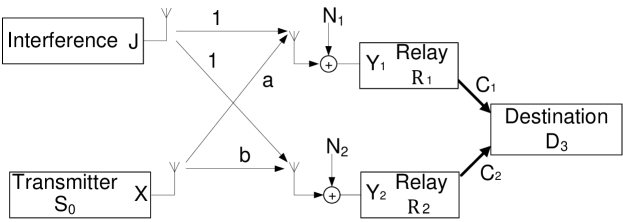
Figure 1: The system setting, with transmitter $S_{0}$ received by $\mathcal{R}_{1}$ and $\mathcal{R}_{2}$ with channel transfer coefficients $a$ and $b$, respectively. Lossless links with respective capacities of $C_{1}$ and $C_{2}$ between relays $\mathcal{R}_{1},\mathcal{R}_{2}$ and destination $\mathcal{D}_{3}$.

The communication system is therefore completely characterized by four deterministic functions ($I_{n}\triangleq[1,\dots,2^{n}]$)

$$\boldsymbol{X}(W)=\phi_{S_{0}}(W) : I_{nR}\rightarrow\mathbb{R}^{n}$$ (3)

$$V_{1}(\boldsymbol{Y}_{1})=\phi_{\mathcal{R}_{1}}(\boldsymbol{Y}_{1}) : \mathbb{R}^{n}\rightarrow I_{nC_{1}}$$ (4)

$$V_{2}(\boldsymbol{Y}_{2})=\phi_{\mathcal{R}_{2}}(\boldsymbol{Y}_{2}) : \mathbb{R}^{n}\rightarrow I_{nC_{2}}$$ (5)

$$\hat{W}(V_{1},V_{2})=\phi_{D_{3}}(V_{1},V_{2}) : I_{nC_{1}}\times I_{nC_{2}}\rightarrow I_{nR}.$$ (6)

We can divide the general case of (1)-(2) into three possible options:

1. $a=0$ or $b=0$, $a\neq b$.

2. $a,b\neq 0,\ a\neq b$.

3. $a=b$.

The last case is of no real interest since the scaling behavior is obvious and remains the same for one or two relays, so this paper will focus only on the first two. Similarly, for $C_{1},C_{2}$ we have three cases, where $C\rightarrow\infty$ means that $C$ goes to infinity much faster than $P_{X},P_{J}$:

1. $C_{1}\rightarrow\infty$ or $C_{2}\rightarrow\infty$.

2. Neither $C_{1}\rightarrow\infty$ nor $C_{2}\rightarrow\infty$.

3. $C_{1}\rightarrow\infty$ and $C_{2}\rightarrow\infty$.

The last case results with full cooperation. In this case the achievable rate and the upper bound are identical and equal to the Shannon capacity, given by (for example for $a=1,b=-1$):

$$R=\frac{1}{2}\log_{2}(1+2P_{X}).$$ (7)

This rate is achieved by using maximal ratio combining of the two receptions, completely eliminating the interference. So the general case in this paper reduces to three main scenarios, in which we investigate the scaling laws of $C_{1}$ and $C_{2}$, as a function of the achievable rate $R$. These three cases consist of the four possible options described above for $a,b,C_{1},C_{2}$, where the option of $C_{1}\rightarrow\infty$ or $C_{1}\rightarrow\infty$ while $ab\neq 0$ was dropped since it is very similar to the case where either $C_{1}\rightarrow\infty$ or $C_{1}\rightarrow\infty$ when $a=0$ or $b=0$ while $a\neq b$.

Since the channel between the transmitter and the relays can support a rate with scaling of up to $\lim_{P_{X}\rightarrow\infty}\frac{R}{\log_{2}(P_{X})}=\frac{1}{2}$, we investigate the required capacities of the links to achieve this scaling, and also the degradation of $R$ when they are smaller.

We denote by scaling the pre-log coefficient defined by the limit $scaling=\lim_{P_{X}\rightarrow\infty}\frac{R}{\log_{2}(P_{X})}$, and write it for the sake of brevity as $R\sim scaling\ \log_{2}(P_{X})$. Similarly, the relation $\lim_{P_{X}\rightarrow\infty}\frac{R}{\log_{2}(P_{X})}\geq\frac{1}{2}$ is designated by $R\gtrsim\frac{1}{2}\log_{2}(P_{X})$.

Case A: Relaying the Interference

The scenario here specializes to

$$a = 1$$ (8)

$$b = 0$$ (9)

$$P_{N_{1}} = 1$$ (10)

$$P_{N_{2}} = 0$$ (11)

$$C_{1} \rightarrow \infty.$$ (12)

The last condition simply states that the destination receives the channel output, which is composed of the transmission plus some unknown interference, which may degrade or even prevent any reliable decoding. The interference is received intact in $\mathcal{R}_{2}$, and then relayed to the destination to enable reliable decoding. We consider a fixed $a=1$ for simplicity. The results for any $a\neq 0$ are obtained from the results for the fixed $a=1$ almost verbatim.

This model can describe a situation where an additive jammer is known to a relay which can assist the destination with resolving the transmission from $S_{0}$. Notice that for an infinite Jammer power ($\frac{P_{J}}{P_{X}}\rightarrow\infty$), a link to the relay $\mathcal{R}_{2}$ is necessary to achieve any positive rate.

Case B: Relaying the Interfered Signal and the Interference

The only change compared to the previous Scenario A is that here $C_{1}$ is finite. The added limitation extends the decentralization inherent in the scheme, which models practical systems where the destination is not collocated near either relays.

Case C: Relaying 2 Interfered Signals

In this scenario we consider the case where

$$a = 1$$ (13)

$$b = -1$$ (14)

$$P_{N_{1}} = 1$$ (15)

$$P_{N_{2}} = 1.$$ (16)

In this case, the signals are in anti-phase and hence joint processing ($C_{1},C_{2}\rightarrow\infty$) via substraction $Y_{1}-Y_{2}$ would completely remove the interference, and would allow for reliable rate of $R=\frac{1}{2}\log_{2}(1+2P_{X})$.
As in the previous cases, the solution to $a=1,b=-1$, gives the same scaling behavior as taking any $a\neq b,\ a\neq 0,\ b\neq 0$. Notice that for scaling, the destination still wants to cancel the interference, and thus still needs to perform $Y_{1}-Y_{2}$, regardless of the actual $a,b$, as long as $a\neq b$. Also the finite $P_{X},P_{J}$ results for this general case are readily derived following the same steps.

III Main Results

The main results described in this Section are divided into the three scenarios detailed above, and include both the achievable rates and outer bounds. The resulting scaling laws of the inner and outer bounds coincide.

Case A: Relaying the Interference

Proposition 1

1. The following rate for Case A is achievable

   $$R\leq\max\left\{\frac{1}{2}\log_{2}\bigg{(}\frac{1+P_{X}}{1+\min\left\{1+P_{X},\frac{P_{J}P_{X}}{P_{X}+1}\right\}2^{-2C_{2}}}\bigg{)},0\right\}.$$ (17)

2. An upper bound for all achievable rates for Case A is (cut-set bound)

   $$R\leq\min\left\{C_{2}+I(X;Y_{1}),I(X;Y_{1}|J)\right\}$$ (18)

   which for the Gaussian channel reads,

   $$R\leq\min\left\{C_{2}+\frac{1}{2}\log_{2}\left(1+\frac{P_{X}}{P_{J}+1}\right),\frac{1}{2}\log_{2}(1+P_{X})\right\}.$$ (19)

The proof of Proposition 1 appears in Section IV, where the achievable rate is just a special case of the achievable rate of Case B. It is understood that the achievable rate (17) is not optimal, but it does prove the scaling laws.

From Proposition 1 the scaling laws can be derived.

Proposition 2

To achieve a scaling of $R\sim\frac{1}{2}\log_{2}(P_{X})$, when relaying the interferer (Case A), the sufficient and necessary lossless link capacity scaling is

$$C_{2}\gtrsim\frac{1}{2}\log_{2}\left(\frac{P_{X}P_{J}}{P_{X}+P_{J}}\right).$$ (20)

Furthermore, the gap between the achievable rate and the upper bound is no more than 1 bit.

This Proposition is proved in Appendix A. The next corollary is a special case of Proposition 2:

Corollary 1

A scaling of $C_{2}\sim\frac{1}{2}\log_{2}(P_{X})$ is sufficient, for any interferer, regardless of its power and statistics.

This Corollary holds, since the proof for the achievable rate in section IV uses random dithering, which achieves the same performance for any $J$ which is independent of the transmitted signal.

For example, when the interferer is another transmitter, the robustness is with respect to the the applied code, modulation technique and interference power. However, the exact phase, between the reception at $Y_{1}$ and $Y_{2}$ is still required.

Case B: Relaying the Interfered Signal and the Interference

Now also $C_{1}$ is finite.

Proposition 3

1. The following rate for Case B is achievable

   $$R<\max\left\{\frac{1}{2}\log_{2}\left(\frac{(1+P_{X})(2^{2C_{1}}-1)}{P_{X}+2^{2C_{1}}+\min\left\{1+P_{X},\frac{P_{J}P_{X}}{P_{X}+1}\right\}2^{-2C_{2}}(2^{2C_{1}}-1)}\right),0\right\}.$$ (21)

2. An upper bound for all achievable rates of Case B is (cut-set bound)

   $$R\leq\min\left\{C_{1},C_{2}+I(X;Y_{1}),I(X;Y_{1}|Y_{2})\right\}$$ (22)

   which for the underlying Gaussian channel turns out to be

   $$R\leq\min\left\{C_{1},C_{2}+\frac{1}{2}\log_{2}\left(1+\frac{P_{X}}{P_{J}+1}\right),\frac{1}{2}\log_{2}(1+P_{X})\right\}.$$ (23)

The proof of Proposition 3 appears in Section IV. It is understood that the achievable rate (21) is not optimal, but it does prove the scaling laws.

Next, we quantify the necessary scaling of the link capacity $C_{1}$.

Proposition 4

To achieve a scaling of $R\sim\frac{1}{2}\log_{2}(P_{X})$, when relaying the interfered signal and the interference (Case B), sufficient and necessary lossless links capacities scale as

$$C_{1} \gtrsim \frac{1}{2}\log_{2}(P_{X})$$ (24)

$$C_{2} \gtrsim \frac{1}{2}\log_{2}\left(\frac{P_{X}P_{J}}{P_{X}+P_{J}}\right).$$ (25)

Furthermore, the gap between the achievable rate and the upper bound is no more than 1.29 bits.

The proof appears in Appendix A.

This Proposition establishes that $C_{1}$, that is the capacity of the link from the relay that receives the signal and the interference to the destination, scales the same as if there was no interference.

Corollary 2

A scaling of $C_{1}\sim\frac{1}{2}\log_{2}(P_{X})$ suffices to achieve robustness against any interference, regardless of its power or statistics, as long as it remains independent of $X$.

In Figure 2, the scaling of the achievable rate of Case B is drawn as a function of $C_{1}+C_{2}$ for $P_{J}<P_{X}$. For the sake of the achievable rate $C_{1},C_{2}$ were selected such that $C_{1}+C_{2}$ is fixed and the achievable rate is maximized. The cut-set upper bound in Case B is met by an achievable rate along the entire range in Figure 2. Specifically, from the point $C_{1}+C_{2}=0$ to $C_{1}+C_{2}=\frac{1}{2}\log_{2}(P_{X}/P_{J})$ ($P2$), an achievable scheme which uses simple local decoding at $\mathcal{R}_{1}$ is optimal. This is since using the decoded information rate equals the cut-set bound ($C_{1}\geq R$), which is therefore tight even for finite $P_{X},P_{J}$. The slope of the curve is 1, since only information bits are forwarded. Such local decoding is optimal as long as $R\leq\frac{1}{2}\log_{2}(1+\frac{P_{X}}{P_{J}+1})$. Higher sum-links-rate benefit by devoting some bandwidth also to the message from $\mathcal{R}_{2}$. The achievable rate of Proposition 3, equation (21) outperforms local decoding. In such scheme both relays basically forward the received signals to the destination, where the signals are subtracted at the destination, which eliminates the interference. Thus every additional forwarded information bit requires also one bit for forwarding the interference. This means that the rate increases only as $\frac{1}{2}(C_{1}+C_{2})$. The outer bound for the range between $P2$ and $C_{1}+C_{2}=\frac{1}{2}\log_{2}(P_{X}P_{J})$ ($P1$) is due to the diagonal cut-set upper bounds ($C_{2}\gtrsim R-\frac{1}{2}\log_{2}\left(1+\frac{P_{X}}{P_{J}}\right)$). The maximal rate is $\frac{1}{2}\log_{2}(P_{X})$, which is reached only when $C_{1}+C_{2}\gtrsim\frac{1}{2}\log_{2}(P_{X}P_{J})$ at $P1$.

Case C: Relaying 2 Interfered Signals

In this case the desired signal is received by both relays along with the common interference.

Proposition 5

1. An achievable rate for Case C is

   $$R>\max\left\{\frac{1}{2}\log_{2}\left(\frac{P_{X}}{\frac{P_{X}}{P_{X}+1}+\frac{P_{X}}{2^{2C_{1}}-1}+\min\{P_{X},P_{J}\frac{P^{2}_{X}}{(P_{X}+1)^{2}}\}2^{-2C_{2}}}\right),0\right\}.$$ (26)

   and this holds also with the indices 1 and 2 interchanged.

2. An upper bound for all achievable rates for Case C is (cut-set bound),

   $$R\leq\min\left\{C_{1}+C_{2},C_{1}+I(X;Y_{2}),C_{2}+I(X;Y_{1}),I(X;Y_{1},Y_{2})\right\}$$ (27)

   which for the underlying Gaussian channel turns out to be

   $$R\leq\min\left\{C_{1}+C_{2},C_{1}+\frac{1}{2}\log_{2}\left(1+\frac{P_{X}}{P_{J}+1}\right),C_{2}+\frac{1}{2}\log_{2}\left(1+\frac{P_{X}}{P_{J}+1}\right),\frac{1}{2}\log_{2}(1+2P_{X})\right\}.$$ (28)

   Another upper bound for all achievable rates for Case C is (Modulo bound)

   $$R\leq\frac{1}{2}\left(C_{1}+C_{2}+\frac{1}{2}\log_{2}\left(1+\frac{P_{X}}{P_{J}}\right)\right)+\frac{1}{4}\log_{2}(8\pi e).$$ (29)

The proof for Proposition 5 appears in Section IV. The achievable rate (26) is not optimal, but it does prove the scaling laws.

Note that (29) states an upper bound for any $R$, including finite rates. However, the bound is interesting only in the case of large $P_{X},P_{J}$, because of the added 1.55 ($\frac{1}{4}\log_{2}(8\pi e)$) bits per channel use.

Proposition 6

Necessary and sufficient conditions on $C_{1},C_{2}$, to achieve the scaling of $R$ when $P_{X},P_{J}$ are taken to infinity are

$$\begin{cases}C_{1}+C_{2}\gtrsim\max\left\{2R-\frac{1}{2}\log_{2}\left(1+\frac{P_{X}}{P_{J}}\right),R\right\}\\ C_{1},C_{2}\gtrsim R-\frac{1}{2}\log_{2}\left(1+\frac{P_{X}}{P_{J}}\right)\end{cases}$$ (30)

Furthermore, the gap between the achievable rate and the outer bound in the asymptotic regime when $R\sim 0.5\log_{2}(P_{X})$ is bounded to 2.816 bits.

The proof of Proposition 6 appears in appendices B and A.

The resulting scaling of the rate region is presented in Figure 3, where the required scaling of $C_{1},C_{2}$, so that the achievable rate has the scaling of $R$ is filled. The bound $B1$ in Figure 3 stands for the bounds on $C_{1}+C_{2}$ such that $C_{1}+C_{2}\gtrsim\max\left\{2R-\frac{1}{2}\log_{2}\left(1+\frac{P_{X}}{P_{J}}\right),R\right\}$, while $B2$ stands for the diagonal bounds, which separately limit $C_{1},C_{2}$ such that $C_{1},C_{2}\gtrsim R-\frac{1}{2}\log_{2}\left(1+\frac{P_{X}}{P_{J}}\right)$. It is evident that any increase of $C_{1}$ or $C_{2}$ can indeed only help, and the rate-region is convex. Achieving the points $P1$ and $P2$, allows to achieve any other point in the interior rate-region, through time sharing.

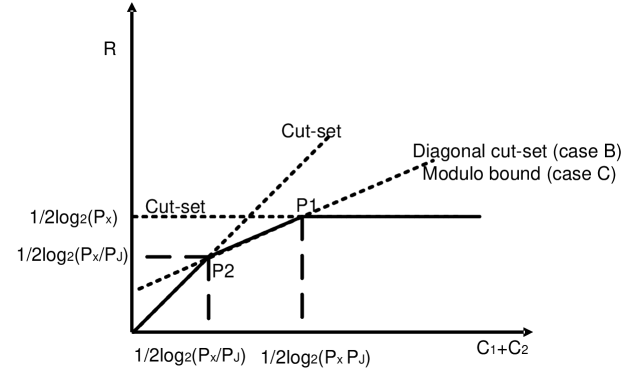
Figure 2: The achievable scaling of the rate $R$ as a function of $C_{1}+C_{2}$, for cases B and C. Upper bounds are drawn with dotted lines, while the full line is the achievable rate. It is evident that the cut-set bound in Case C is not tight, and the modulo bound was needed to characterize the scaling laws. For Case B, the cut-set bound is tight for the whole region.

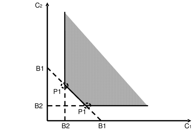
Figure 3: The scaling of $C_{1},C_{2}$ as a function of the achievable rate $R$, where $B1$ is the scaling of $\max\left\{2R-\frac{1}{2}\log_{2}\left(1+\frac{P_{X}}{P_{J}}\right),R\right\}$ and $B2$ is the scaling of $R-\frac{1}{2}\log_{2}\left(1+\frac{P_{X}}{P_{J}}\right)$. The filled area denotes $C_{1}$ and $C_{2}$ which enable communication at rate $R$.

In Figure 2, the scaling of the achievable rate is drawn as a function of the scaling of $C_{1}+C_{2}$, when $C_{1}=C_{2}$, letting $P_{J}<P_{X}$. From the point $(0,0)$ to $P2$, an achievable scheme uses simple local decoding at the relays. Since this scheme uses all the links’ bandwidth to forward only decoded information, the cut-set bound is tight, and the slope of the curve is 1. Such local decoding is possible as long as $R\lesssim\frac{1}{2}\log_{2}(1+\frac{P_{X}}{P_{J}})$. Achieving higher rates requires more than local decoding, and the achievable rate of Proposition 5, equation (26) is used. The outer bound for this range is due to the modulo outer bound (29). This scheme basically forwards the received signals to the destination, where the signals are subtracted to eliminate the interference. As in Case B, we get rid of the interference only at the destination, which means that the rate scaling increases only as the scaling of $\frac{1}{2}(C_{1}+C_{2})$. The maximal rate scaling is $\frac{1}{2}\log_{2}(P_{X})$, which is reached only when $C_{1}+C_{2}\gtrsim\frac{1}{2}\log_{2}(P_{X}P_{J})$ at $P1$. The modulo bound (29) determines the behavior between the points $P2$ and $P1$.

Corollary 3

The cut-set upper bound is strictly loose for the interference channel of Case C.

Proof:

Take $P_{J}=\sqrt{P_{X}}$ and $C_{1}=C_{2}=\frac{1}{4}\log_{2}(P_{X})$. Then the cut-set bound from Equation (27) for the scaling reads $R\gtrsim R_{cut}=\frac{1}{2}\log_{2}(P_{X})$, while the modulo bound of Equation (29) for the scaling reads $R\gtrsim R_{mod}=\frac{1}{4}\log_{2}(P_{X})$. So we showed that $R_{cut}>R_{mod}+\epsilon$ for some $\epsilon>0$. ∎

Remark 1

For cases A and B, when considering the outer bound due to the underlying Gaussian channel, $R\leq\frac{1}{2}\log_{2}(1+P_{X})$ and combining propositions 2 and 4 we get that for large $P_{X},P_{J}$, $\frac{1}{n}H(V_{2})\gtrsim\frac{1}{2}\log_{2}\left(\frac{P_{X}P_{J}}{P_{X}+P_{J}}\right)$. By adding also that $H(V_{2}|\boldsymbol{J})=0$ since $V_{2}$ is a deterministic function of $\boldsymbol{J}$, it follows that

$$\frac{1}{n}I(V_{2};\boldsymbol{J})\gtrsim\frac{1}{2}\log_{2}\left(\frac{P_{X}P_{J}}{P_{X}+P_{J}}\right).$$ (31)

So that in order to achieve a reliable rate $R\sim\frac{1}{2}\log_{2}(P_{X})$, a defined amount of information about the interferer is required at the destination with scaling $\frac{1}{2}\log_{2}\min\{P_{X},P_{J}\}$, for large $P_{X},P_{J}$.

IV Proofs for Basic Propositions

In this section we prove the basic propositions, not the propositions dealing with the scaling laws, which appear in appendices A-B.

IV-A Proofs for the Outer Bounds

In this section we present the proofs of the necessary conditions of the propositions in Section III.

Proof of Outer Bounds for Cases A,B and C in equations (18),(22) and (27): The cut-set outer bound [27] is simply the minimum among all the communication rates between any two cuts of the network [27] as is reflected in the three cases under study. Let us show the cut-set for one such cut, for the sake of conciseness, where the rest of the cuts readily follow. Take the cut such that one set includes the transmitter with relay $\mathcal{R}_{1}$ and therefore the other set includes $\mathcal{R}_{2}$ and the destination. From [27], Theorem 14.10.1: The achievable rate must be less than or equal to $I(X^{(S)};Y^{(S^{c})}|X^{(S^{c})})$ for some single letter joint probability distribution $P(X^{(S)},X^{(S^{c})})$. In our setting with the chosen cut, $X^{(S)}=(X,V_{1})$, $Y^{(S^{c})}=(Y_{2},V_{1})$ and $X^{(S^{c})}=V_{2}$, since the destination can not transmit anything. The underlying channel is $P(Y^{(S^{c})}|X^{(S^{c})},X^{(S)})=P(Y_{2},V_{1}|X,V_{1},V_{2})=P(Y_{2}|X)$. The right-most equality is since $Y_{2}$ is not affected by $V_{1}$ or $V_{2}$, and the resulting Markov chain is $V_{1}-X-Y_{2}$.

To get the upper bound we need to maximize $I(X,V_{1};Y_{2},V_{1}|V_{2})$ over $P(X,V_{1},V_{2})$. The mutual information $I(X,V_{1};Y_{2},V_{1}|V_{2})$ is determined only by $P(X,V_{1},V_{2})$ and by the given channel $P(Y_{1},Y_{2}|X)$ such that $I(X,V_{1};Y_{2},V_{1}|V_{2})=I(X,V_{1};Y_{2},V_{1})$. Since $V_{1}-X-Y_{2}$ is a Markov chain:

$$I(X,V_{1};Y_{2},V_{1})=H(V_{1},X)-H(X|V_{1},Y_{2})=H(V_{1}|X)+I(X;V_{1},Y_{2})=\\ =H(V_{1}|X)+I(Y_{2};X)+H(V_{1}|Y_{2})-H(V_{1}|Y_{2},X)$$ (32)

Due to the Markov chain above, $H(V_{1}|Y_{2},X)=H(V_{1}|X)$. So that

$$R\leq I(Y_{2};X)+H(V_{1}|Y_{2})\leq I(Y_{2};X)+C_{1}.$$ (33)

Considering all the cut-sets, equation (18) follows from

$$R\leq\min\left\{C_{2}+I(X;Y_{1}),I(X;Y_{1},Y_{2})\right\}=\min\left\{C_{2}+I(X;Y_{1}),I(X;Y_{1}|Y_{2})+I(X;Y_{2})\right\}\\ =\min\left\{C_{2}+I(X;Y_{1}),I(X;Y_{1}|J)\right\}$$ (34)

where the last equality follows since $Y_{2}=J$. The complete proofs for the inequalities in equations (22) and (28) are omitted here since they are proved exactly the same way. ∎

Proof of the Modulo Outer Bound in Case C (29):
The basis of the proof is the representation of the transmitted signal ($X$) by two components, one is an integer which is basically known at the relays (with high probability), and the other is a heavily interfered real signal.
Definition: For any $X$, $X^{-}\triangleq X\mod\sqrt{P_{J}}$ and $X^{+}\triangleq\left\lfloor\frac{X}{\sqrt{P_{J}}}\right\rfloor$.

Assuming, without loss of any generality, that

$$H(V_{1}|\boldsymbol{X}^{+},V_{2})\leq H(V_{2}|\boldsymbol{X}^{+},V_{1}).$$ (35)

If (35) is not satisfied, replace the indices of 1 and 2 in the following. Using Fano’s inequality, where $\epsilon>0$ is arbitrary small, for sufficiently large $n$, we get that

$$nR \leq I(\boldsymbol{X};V_{1},V_{2})+n\epsilon$$ (36)

$$= I(\boldsymbol{X}^{+};V_{1},V_{2})+I(\boldsymbol{X}^{-};V_{1},V_{2}|\boldsymbol{X}^{+})+n\epsilon$$ (37)

$$= I(\boldsymbol{X}^{+};V_{1},V_{2})+I(\boldsymbol{X}^{-};V_{1}|\boldsymbol{X}^{+},V_{2})+I(\boldsymbol{X}^{-};V_{2}|\boldsymbol{X}^{+})+n\epsilon$$ (38)

$$\leq I(\boldsymbol{X}^{+};V_{1},V_{2})+H(V_{1}|\boldsymbol{X}^{+},V_{2})+I(\boldsymbol{X}^{-};\boldsymbol{Y}_{2}|\boldsymbol{X}^{+})+n\epsilon$$ (39)

$$\leq I(\boldsymbol{X}^{+};V_{1},V_{2})+\frac{1}{2}[H(V_{1}|\boldsymbol{X}^{+},V_{2})+H(V_{2}|\boldsymbol{X}^{+})]+h(\boldsymbol{Y}_{2}|\boldsymbol{X}^{+})-h(\boldsymbol{Y}_{2}|\boldsymbol{X})+n\epsilon$$ (40)

$$\leq I(\boldsymbol{X}^{+};V_{1},V_{2})+\frac{1}{2}H(V_{1},V_{2}|\boldsymbol{X}^{+})+h(-\boldsymbol{X}^{-}+\boldsymbol{J}+\boldsymbol{N}_{2})-h(\boldsymbol{J}+\boldsymbol{N}_{2})+n\epsilon$$ (41)

$$= I(\boldsymbol{X}^{+};V_{1},V_{2})+\frac{1}{2}[H(V_{1},V_{2})-I(\boldsymbol{X}^{+};V_{1},V_{2})]+I(\boldsymbol{X}^{-};-\boldsymbol{X}^{-}+\boldsymbol{J}+\boldsymbol{N}_{2})+n\epsilon$$ (42)

$$\leq \frac{1}{2}I(\boldsymbol{X}^{+};V_{1},V_{2})+\frac{1}{2}H(V_{1},V_{2})+\frac{n}{2}\log_{2}\left(1+\frac{P_{J}}{1+P_{J}}\right)+n\epsilon$$ (43)

$$\leq \frac{n}{4}\log_{2}\left(2\pi e\left(\frac{P_{X}}{P_{J}}+\frac{1}{12}\right)\right)+\frac{n}{2}(C_{1}+C_{2})+\frac{n}{2}\log_{2}\left(1+\frac{P_{J}}{1+P_{J}}\right)+n\epsilon.$$ (44)

Where (39) is since $H(V_{1}|\boldsymbol{X},V_{2})\geq 0$, and the data processing Lemma $V_{2}=\phi_{\mathcal{R}_{2}}(Y_{2})$, (40) follows from (35) and by writing the mutual information as the difference between two entropies, (41) is since $h(X^{-}+J+N_{2}|X^{+})\leq h(X^{-}+J+N_{2})$ and $h(Y_{2}|X)=h(J+N_{2})$, (42) is by noticing that $h(J+N_{2})=h(X^{-}+J+N_{2}|X^{-})$ and simply writing the difference between the entropies as mutual information, (43) is because $\mathrm{E}|X^{-}|^{2}\leq P_{J}$ and finally (44) is since $H(V_{1},V_{2})\leq C_{1}+C_{2}$ and $I(\boldsymbol{X}^{+};V_{1},V_{2})\leq H(\boldsymbol{X}^{+})$, where $\mathrm{E}|\boldsymbol{X}^{+}|^{2}\leq\frac{P_{X}}{P_{J}}$, and using Theorem 9.7.1 from [27].

∎

IV-B Proofs for the Achievable Rate

Proof for Cases B and C (Propositions 3 and 5):
Here we avoid reconstructing the whole $J$ at the destination by utilizing a lattice code and reducing the signals into its Voronoi cell by a modulo operation. Our scheme is an adaptation of the MLAN channel technique from [17].

First define the lattice code $\mathbb{C}_{2}$ which is a good source $P_{X}$-code, which means that it satisfies, for any $\varepsilon>0$ and adequately large lattice dimension $n$

$$\begin{split}\log(2\pi eG(\mathbb{C}_{2}))<\varepsilon\\ P_{X}=\frac{\int_{\nu_{2}}||\mathbf{x}||^{2}d\mathbf{x}}{V_{o}n}.\end{split}$$ (45)

Where $G(\mathbb{C}_{2})$, $\nu_{2}$ and $V_{o}$ are the normalized second moment, the Voronoi cell and the Voronoi cell volume of the lattice associated with $\mathbb{C}_{2}$, respectively. Such codes are known to exist [16].

1. Transmission Scheme: Transmit the information $W$ as a codeword from a codebook, where every codeword in this codebook is randomly and independently generated by dividing it into many (multi-letter) entries, each generated uniformly i.i.d. over the Voronoi region of $\mathbb{C}_{2}$, $\nu_{2}$. Define the transmitted codeword as $V$. Add a pseudo random dithering $-U$, which is uniformly generated over $\nu_{2}$ and known to all parties, to get: $X=V-U\mod\mathbb{C}_{2}$ (modulo Voronoi region of $\mathbb{C}_{2}$). This dither is required for the analysis, to ensure independence of the modulo noise with respect to the message index.

2. Relaying Scheme: Both relays $\mathcal{R}_{1}$ and $\mathcal{R}_{2}$ multiply the received signals by $\alpha>0$, apply $\mod\mathbb{C}_{2}$, and quantize the received signal using standard information theory techniques into $W_{1}=\alpha Y_{1}\mod\mathbb{C}_{2}+D_{1}$ and $W_{2}=\alpha Y_{2}\mod\mathbb{C}_{2}+D_{2}$. The quantization is given in Appendix C, where $U$,$Y$ in Appendix C are $W_{1}=\alpha Y_{1}\mod\mathbb{C}_{2}+D_{1}$ and $\alpha Y_{1}\mod\mathbb{C}_{2}$, respectively. The underlying single letter distortions $D_{1}$ and $D_{2}$ in $W_{1},W_{2}$ are Gaussian with zero mean and are independent with any other random variable.

   A Slepian Wolf encoding is then used on the two vector quantized signals, before transmission to the destination.

3. Decoding at Destination: Now the destination decodes $W_{1}$ and $W_{2}$ and calculates $W_{1}-W_{2}$. From the result, it further subtracts the known pseudo random dither $U$, and applies again modulo $\mathbb{C}_{2}$ (see equation (48)). It then finds the vector $\hat{V}$ which is jointly typical with the resulting outcomes of the modulo operation. The decoded message is the corresponding message index $W$, if decoding is successful.

4. Analysis of Performance: The independent distortion variance $P_{D_{1}}$ corresponds to what is promised by the rate distortion function for any random variable with variance of $P_{X}$, and in particular, to $\alpha Y_{1}\mod\mathbb{C}_{2}$ (See Appendix C for the complete proof). The rate for independent distortion for $Y_{1}$ is

   $$I(W_{1};\alpha Y_{1}\mod\mathbb{C}_{2})=\frac{1}{2}\log\frac{P_{X}+P_{D_{1}}}{P_{D_{1}}}\leq C_{1}.$$ (46)

   Notice that taking $D_{1}$ such that $P_{D_{1}}$ fulfills (46) allow us to chose $D_{1}$ to be distributed independently of $\alpha Y_{1}\mod\mathbb{C}_{2}$, regardless of $\alpha$.

   For Proposition 3: Depending on whether $\alpha^{2}P_{J}<P_{X}$ or $\alpha^{2}P_{J}>P_{X}$, using the result in Appendix C, we get for $P_{D_{2}}$

   $$I(W_{2};\alpha Y_{2}\mod\mathbb{C}_{2})=\frac{1}{2}\log\frac{\min\{P_{X},\alpha^{2}P_{J}\}}{P_{D_{2}}}\leq C_{2}.$$ (47)

   Since $X=V-U$, we can write $\alpha Y_{1}-\alpha Y_{2}+U=\alpha X+\alpha N_{1}+U=X+U-(1-\alpha)X+\alpha N_{1}=V-(1-\alpha)X+\alpha N_{1}$, and the following equalities hold

   $$Y = W_{1}-W_{2}+U\mod\mathbb{C}_{2}$$ (48)

   $$= \alpha Y_{1}+D_{1}-\alpha Y_{2}-D_{2}+U\mod\mathbb{C}_{2}$$ (49)

   $$= V-(1-\alpha)X+\alpha N_{1}+D_{1}-D_{2}\mod\mathbb{C}_{2}.$$ (50)

   Define

   $$N_{eq}=\alpha N_{1}+D_{1}-D_{2}-(1-\alpha)X.$$ (51)

   with

   $$P_{N_{eq}}=\alpha^{2}P_{N_{1}}+(1-\alpha)^{2}P_{X}+P_{D_{1}}+P_{D_{2}}.$$ (52)

   Encoding according to $V$ which is uniformly distributed over $\mathbb{C}_{2}$ gives an achievable rate of (See Inflated Lattice Lemma in [17])

   $$R>\frac{1}{n}\left(\log_{2}\frac{V_{o}}{G(\mathbb{C}_{2})}-H(N_{eq})\right)-\delta=\frac{1}{2}\log_{2}(2\pi eP_{X})-\frac{1}{2}\log_{2}\left(2\pi eP_{N_{eq}}\right)-\delta.$$ (53)

   Setting $\alpha$ to maximize the achievable rate

   $$\alpha=\frac{P_{X}}{P_{X}+P_{N_{1}}},$$ (54)

   along with (46) and (47) results in

   $$R>\frac{1}{2}\log_{2}\left(\frac{P_{X}}{\frac{P_{X}P_{N_{1}}}{P_{X}+P_{N_{1}}}+P_{D_{1}}+P_{D_{2}}}\right)-\delta=\frac{1}{2}\log_{2}\left(\frac{P_{X}}{\frac{P_{X}P_{N_{1}}}{P_{X}+P_{N_{1}}}+\frac{P_{X}}{2^{2C_{1}}-1}+\min\{P_{X},P_{J}\frac{P^{2}_{X}}{(P_{X}+P_{N_{1}})^{2}}\}2^{-2C_{2}}}\right)-\delta.$$ (55)

   Considering that $P_{N_{1}}=1$, after some simple algebra, (55) becomes (21). ∎

For Proposition 5: On one hand

$$\frac{1}{n}H(\mathbb{W_{2}}|\mathbb{W_{1}})\leq\frac{1}{n}H(\mathbb{W_{2}})\leq\frac{1}{2}\log\left(1+\frac{P_{X}}{P_{D_{2}}}\right),$$ (56)

on the other hand

$$\frac{1}{n}H(\mathbb{W_{2}}|\mathbb{W_{1}})=\frac{1}{n}H(\mathbb{W_{1}}+\mathbb{W_{2}}|\mathbb{W_{1}})\leq\frac{1}{n}H(\mathbb{W_{1}}+\mathbb{W_{2}})\leq\frac{1}{2}\log\left(1+\frac{\alpha^{2}(4P_{J}+P_{N_{1}}+P_{N_{2}})+P_{D_{1}}}{P_{D_{2}}}\right).$$ (57)

So for a successful Slepian-Wolf decoding we require that the minimum between the right hand sides of equations (56) and (57) be smaller than $C_{2}$. This brings us to

$$\frac{1}{2}\log\left(1+\frac{\min\{P_{X},\alpha^{2}(4P_{J}+P_{N_{1}}+P_{N_{2}})+P_{D_{1}}\}}{P_{D_{2}}}\right)\leq C_{2}.$$ (58)

As in (50), here we have

$$Y=V-(1-2\alpha)X+\alpha(N_{1}+N_{2})+D_{1}+D_{2}\mod\mathbb{C}_{2}.$$ (59)

and $P_{N_{eq}}$ in this case, is

$$P_{N_{eq}}=\alpha^{2}(P_{N_{1}}+P_{N_{2}})+(1-2\alpha)^{2}P_{X}+P_{D_{1}}+P_{D_{2}}.$$ (60)

Taking

$$\alpha=\frac{2P_{X}}{4P_{X}+P_{N_{1}}+P_{N_{2}}},$$ (61)

we get (considering that $P_{N_{1}}=P_{N_{2}}=1$)

$$R>\frac{1}{2}\log_{2}\left(\frac{P_{X}}{\frac{P_{X}(P_{N_{1}}+P_{N_{2}})}{4P_{X}+P_{N_{1}}+P_{N_{2}}}+P_{D_{1}}+P_{D_{2}}}\right)-\delta\geq\frac{1}{2}\log_{2}\left(\frac{P_{X}}{\frac{1}{2}+\frac{P_{X}}{2^{2C_{1}}-1}+\frac{\min\{P_{X},4P_{J}+2+\frac{P_{X}}{2^{2C_{1}}-1}\}}{2^{2C_{2}}-1}}\right)-\delta.$$ (62)

The proof can be further replicated also when interchanging the indices 1 and 2. ∎

V Conclusions and Discussions

In this paper, we derive both inner and outer bounds of the communication rate, for three common distributed reception scenarios, with unknown interference. The three scenarios characterize the very low noise case of the more general case of distributed reception of wanted signal plus unknown interference. The inner bounds rely on lattice coding, since standard random coding techniques do not provide satisfactory results, in general. Outer bounds based on the cut-set technique are derived, and additional tighter bound is derived by using multi-letter techniques, for a case where the cut-set bound does not suffice. This case includes two relays, which receive both the desired signal and the interference. The generally loose inner and outer bounds which coincide at asymptotically large powers of the transmitter and the interferer, are used to derive the scaling laws. These scaling laws reveal that in order to overcome interference, a defined amount of information about the interference must be known at the destination. The proposed scheme for the inner bound, is also robust against the interference statistics, code, modulation etc.
The model is intimately related to the case of two independent transmitters. Then the transmission of one transmitter can be treated as interference with power $P_{J}$ as in this paper. This approach is beneficial when the rate in which the interfering transmitter $R_{J}$ is high, so codebook knowledge is useless. If in addition the power of the interfering transmitter is high $P_{J}>P_{X}$, then the achievable rates in this paper provide a better approach than the standard compress-and-forward.

Appendix A Proofs for the asymptotic gaps

Define the gap between the achievable rate and the outer bound as $\Delta$.

A-A Case A

For Case A, where $C_{2}=\frac{1}{2}\log_{2}(1+P_{X})$ and $P_{J}>P_{X}$ we get

$$\Delta=C_{2}+\frac{1}{2}\log_{2}\left(1+\frac{P_{X}}{P_{J}+1}\right)-\frac{1}{2}\log_{2}\bigg{(}\frac{1+P_{X}}{1+\min\left\{1+P_{X},\frac{P_{J}P_{X}}{P_{X}+1}\right\}2^{-2C_{2}}}\bigg{)}\leq\\ \frac{1}{2}\log_{2}\left(1+\frac{P_{X}}{P_{J}+1}\right)+\frac{1}{2}\log_{2}(2)\leq\frac{1}{2}\log_{2}(1.5\times 2)=0.7925,$$ (63)

whereas for $P_{J}<P_{X}$ and $C_{2}=\frac{1}{2}\log_{2}(P_{J})$ we get

$$\Delta=C_{2}+\frac{1}{2}\log_{2}\left(1+\frac{P_{X}}{P_{J}+1}\right)-\frac{1}{2}\log_{2}\bigg{(}\frac{1+P_{X}}{1+\min\left\{1+P_{X},\frac{P_{J}P_{X}}{P_{X}+1}\right\}2^{-2C_{2}}}\bigg{)}\leq\\ \frac{1}{2}\log_{2}\left(P_{J}+P_{X}\right)-\frac{1}{2}\log_{2}\bigg{(}\frac{1+P_{X}}{1+\frac{P_{X}}{P_{X}+1}}\bigg{)}\leq\frac{1}{2}\log_{2}(2*2)=1.$$ (64)

So overall for Case A, $\Delta\leq 1$.

A-B Case B

For Case B, where $C_{1}=\frac{1}{2}\log_{2}(1+P_{X})$,$C_{2}=\frac{1}{2}\log_{2}(P_{J})$ and $P_{X}>1$, we get that

$$\min\left\{1+P_{X},\frac{P_{J}P_{X}}{P_{X}+1}\right\}2^{-2C_{2}}(2^{2C_{1}}-1)\leq 1+P_{X}.$$ (65)

Which gives

$$\Delta=C_{2}+\frac{1}{2}\log_{2}\left(1+\frac{P_{X}}{P_{J}+1}\right)-\frac{1}{2}\log_{2}\left(\frac{(1+P_{X})(2^{2C_{1}}-1)}{P_{X}+2^{2C_{1}}+\min\left\{1+P_{X},\frac{P_{J}P_{X}}{P_{X}+1}\right\}2^{-2C_{2}}(2^{2C_{1}}-1)}\right)\leq\\ \frac{1}{2}\log_{2}\left(P_{J}+P_{X}\right)-\frac{1}{2}\log_{2}\left(\frac{(1+P_{X})P_{X}}{P_{X}+(1+P_{X})+(1+P_{X})}\right)\leq\\ \frac{1}{2}\log_{2}(2)+\frac{1}{2}\log_{2}\left(P_{X}\right)-\frac{1}{2}\log_{2}\left(\frac{P_{X}}{3}\right)\leq 1.29.$$ (66)

So overall for Case B, $\Delta\leq 1.29$.

A-C Case C

For Case C, where $P_{J}<P_{X}<\frac{(1+P_{X})^{2}}{P_{X}}$, the modulo upper bound is relevant. So we have

$$\Delta=\frac{1}{2}\left(C_{1}+C_{2}+\frac{1}{2}\log_{2}\left(1+\frac{P_{X}}{P_{J}}\right)\right)+\frac{1}{4}\log_{2}(8\pi e)\\ -\frac{1}{2}\log_{2}\left(\frac{P_{X}}{\frac{P_{X}}{P_{X}+1}+\frac{P_{X}}{2^{2C_{1}}-1}+P_{J}\frac{P_{X}}{(P_{X}+1)^{2}}2^{-2C_{2}}}\right).$$ (67)

We evaluate the gap for corner case where we take $C_{1}=\frac{1}{2}\log_{2}(1+P_{X})$ and $C_{2}=\frac{1}{2}\log_{2}(P_{J})$.

$$\Delta=\frac{1}{2}\left(\frac{1}{2}\log_{2}(1+P_{X})+\frac{1}{2}\log_{2}(P_{J})+\frac{1}{2}\log_{2}\left(1+\frac{P_{X}}{P_{J}}\right)\right)+\frac{1}{4}\log_{2}(8\pi e)\\ -\frac{1}{2}\log_{2}\left(\frac{P_{X}}{\frac{P_{X}}{P_{X}+1}+\frac{P_{X}}{P_{X}}+\frac{P_{X}}{(P_{X}+1)^{2}}}\right).$$ (68)

Since $\frac{P_{X}}{P_{X}+1}+1+\frac{P_{X}}{(P_{X}+1)^{2}}=\frac{P_{X}(1+P_{X})+(1+P_{X})^{2}+P_{X}}{(P_{X}+1)^{2}}\leq 3$, (68) using $P_{J}>1$ gives

$$\Delta\leq\frac{1}{4}\log_{2}(4)+\frac{1}{2}\log_{2}(P_{X})+\frac{1}{4}\log_{2}(8\pi e)-\frac{1}{2}\log_{2}\left(\frac{P_{X}}{3}\right)=\frac{1}{4}\log_{2}(8\times 4\times 9\pi e)=2.816.$$ (69)

For $P_{J}>\frac{(1+P_{X})^{2}}{P_{X}}$, the relevant upper bound is the cut-set bound. We find the gap for $C_{1}=C_{2}=\frac{1}{2}\log_{2}(1+P_{X})$, which gives the correct scaling. So here we have (also using $P_{X}>1$):

$$\Delta=C_{1}+\frac{1}{2}\log_{2}\left(1+\frac{P_{X}}{P_{J}+1}\right)-\frac{1}{2}\log_{2}\left(\frac{P_{X}}{\frac{P_{X}}{P_{X}+1}+\frac{P_{X}}{2^{2C_{1}}-1}+P_{X}2^{-2C_{2}}}\right)\leq\\ C_{1}+\frac{1}{2}\log_{2}\left(2\right)-\frac{1}{2}\log_{2}\left(\frac{P_{X}}{\frac{P_{X}}{P_{X}+1}+1+\frac{P_{X}}{1+P_{X}}}\right)\leq\frac{1}{2}\log_{2}(2\times 4)=1.5.$$ (70)

So overall, in the low noise power limit, when $R\sim 0.5$, for cases A,B and C the gap between the achievable rate and the outer bound is bounded to 1,1.29 and 2.816 bits, respectively.

Appendix B Proof for scaling laws of Case C

Proof:

Necessary conditions: The outer bound in (28),(29) is written as a rate region for $C_{1},C_{2}$ in (30), such that four constraints are met, where two constraints limit $C_{1}+C_{2}$ and the other two constraints limit $C_{1}$ and $C_{2}$ separately.
Sufficient conditions: The outer bound (30) consists of three inequalities, which leads to two intersections points (see Figure 3). Thus the entire region is achievable, for example by using time sharing, provided the point where the capacities of the links are $C_{1}\sim\max\left\{R,\frac{1}{2}\log_{2}\left(1+\frac{P_{X}}{P_{J}}\right)\right\},C_{2}\sim R-\frac{1}{2}\log_{2}\left(1+\frac{P_{X}}{P_{J}}\right)$ (P1 in Figure 3) corresponds to a scheme with the same scaling of the reliable rate as $R$. The proof is then completed by repeating the same arguments for the second point (P2 in Figure 3).

In case $R\lesssim\frac{1}{2}\log_{2}\left(1+\frac{P_{X}}{P_{J}+1}\right)$, use $P_{X}$ to transmit so that the message will be separately decoded at the agents, where $C_{1}=R$ and $C_{2}=0$. Since the agents receive the transmitted signal with signal to noise plus interference ratio of $\frac{P_{X}}{P_{J}+1}$, decoding is reliable. In case $R\gtrsim\frac{1}{2}\log_{2}\left(1+\frac{P_{X}}{P_{J}}\right)$, use the scheme from Proposition 5, which achieves the rate of (26), with $C_{1}\sim R$ and $C_{2}\sim R-\frac{1}{2}\log_{2}\left(1+\frac{P_{X}}{P_{J}}\right)$. This rate is

$$\frac{1}{2}\log_{2}\left(\frac{P_{X}}{P_{X}2^{-2C_{1}}+\min\{P_{X},P_{J}\}2^{-2C_{2}}}\right)=\frac{1}{2}\log_{2}\left(2^{2R}\frac{P_{X}}{P_{X}+\min\{P_{X},P_{J}\}(1+\frac{P_{X}}{P_{J}})}\right)\sim R.$$ (71)

The bounded gap between the achievable rate and the upper bound is evaluated in Appendix A. ∎

Appendix C Proof for compression

Proof that $R>I(Y;U)$ is sufficient for the relay which received $Y$ to forward $U$ to the final destination. For any $\epsilon>0$,

1. Preliminaries As is commonly done (see [27], section 13.6), define the $\epsilon$-typical set $\mathbf{T}_{\epsilon}$ of vectors $\boldsymbol{a}_{1,2}$, with relation to the probability density function $P_{a_{1,2}}$ as

   $$\mathbf{T}_{\epsilon}\triangleq\ \Bigg{\{}\boldsymbol{a}_{1,2}:\ \forall\mathcal{S}\subseteq\{1,2\},\ \left|-\frac{1}{n}\log_{2}\left(P^{n}_{a_{\mathcal{S}}}(\boldsymbol{a}_{\mathcal{S}})\right)-h(P_{a_{\mathcal{S}}})\right|<\epsilon,\Bigg{\}}$$ (72)

   where $P^{n}_{a_{\mathcal{S}}}(\boldsymbol{a}_{\mathcal{S}})=\prod_{i=1}^{n}P_{a_{\mathcal{S}}}\left((\boldsymbol{a}_{\mathcal{S}})_{i}\right)$, and $h(P_{a_{\mathcal{S}}})$ is the differential entropy of the probability density function $P_{a_{\mathcal{S}}}$, where $\mathcal{S}=[1,2,\{1,2\}]$.

   Lemma 1

   (AEP) For any $\epsilon>0$, there exist $n^{*}$ such that for all $n>n^{*}$ and $\boldsymbol{a}_{1,2}\sim\prod P_{A_{1,2}}$ we have

   $$P(\boldsymbol{a}_{1,2}\in\mathbf{T}_{\epsilon})\geq 1-\epsilon.$$ (73)

   Proof:

   See [27] Theorem 9.2.2. ∎

   Lemma 2

   Let $\boldsymbol{a}_{1,2}$ be generated according to

   $$\boldsymbol{a}_{1,2}\sim\prod_{i=1}^{n}P_{a_{1}}((\mathbf{a}_{1})_{i})P_{a_{2}}((\mathbf{a}_{2})_{i}).$$ (74)

   Then we have

   $$\Pr(\boldsymbol{a}_{1,2}\in\mathbf{T}_{\epsilon})=\frac{\Pr(\boldsymbol{a}_{1,2}\in\mathbf{T}_{\epsilon}\bigcup\boldsymbol{a}_{1}\in\mathbf{T}_{\epsilon}\bigcup\boldsymbol{a}_{2}\in\mathbf{T}_{\epsilon})}{\Pr(\boldsymbol{a}_{1}\in\mathbf{T}_{\epsilon})\Pr(\boldsymbol{a}_{2}\in\mathbf{T}_{\epsilon})}\geq 2^{-n[h(a_{1})+h(a_{2})-h(a_{1,2})+\epsilon_{1}]}=2^{-n[I(a_{1};a_{2})+\epsilon_{1}]}$$ (75)

   where $\epsilon_{1}\rightarrow 0$ as $\epsilon\rightarrow 0$.
   

2. Code generation Randomly generate $2^{nI(Y;U)}$ codewords $\mathbf{U}$, according to i.i.d. distribution $\Pi_{i=1}^{n}P_{U}(U_{i})$. Index these codewords by $z\in[1,2^{nI(Y;U)}]$. The codebook is made available to the relay and the destination.

3. Compression After receiving the vector $\mathbf{Y}$, the relay searches for $z$ such that $\{\mathbf{U}(z),\mathbf{Y}\}\in\mathbf{T}_{\epsilon}$. If no such $z$ is found, the relay sends $z=1$.

4. Error Analysis The probability of two independent random variables $\mathbf{U},\mathbf{Y}$ to be jointly typical is lower bounded by

   $$2^{-n[I(Y;U)+\epsilon]}.$$ (76)

   Thus the probability that no such $z$ is jointly typical is upper bounded by

   $$\left(1-2^{-n[I(Y;U)+\epsilon]}\right)^{2^{nR}},$$ (77)

   which tend to zero as $n$ gets large as long as $R>I(Y;U)+\epsilon$. ∎

References

- [1] A. Sanderovich, S. Shamai, Y. Steinberg, and G. Kramer, “Communication via decentralized processing,” IEEE Trans. Inform. Theory, vol. 54, no. 7, pp. 3008–3023, July 2008.
- [2] A. Sanderovich, O. Somekh, V. Poor, and S. Shamai, “Uplink macro diversity of limited backhaul cellular network,” IEEE Trans. Inform. Theory, vol. 55, no. 8, pp. 3457 – 3478, Aug. 2009.
- [3] A. Sanderovich, O. Somekh, and S. Shamai, “Uplink macro diversity with limited backhaul capacity,” in Proc. of IEEE Int. Symp. Info. Theory (ISIT2007), Nice, France, June 2007, pp. 11–15.
- [4] A. Sanderovich, S. Shamai, and Y. Steinberg, “Distributed MIMO receiver - achievable rates and upper bounds,” IEEE Trans. Inform. Theory, vol. 55, no. 10, pp. 4419 – 4438, Oct. 2009.
- [5] G. Hedby, “Error bounds for the euclidean channel subject to intentional jamming,” IEEE Trans. Inform. Theory, vol. 40, no. 2, pp. 594–600, March 1994.
- [6] E. Tekin and A. Yener, “The general Gaussian multiple-access and two-way wire-tap channels: Achievable rates and cooperative jamming,” IEEE Trans. Inform. Theory, vol. 54, no. 6, pp. 2735 – 2751, June 2008.
- [7] I. Maric, R. Dabora, and A. Goldsmith, “Generalized relaying in the presence of interference,” in 42nd Asilomar Conference on Signals, Systems and Computers, Oct. 2008, pp. 1579 – 1582.
- [8] ——, “On the capacity of the interference channel with a relay,” in IEEE International Symposium on Information Theory, Toronto, Ontario, Canada, July 2008, pp. 554 – 558.
- [9] R. Dabora, I. Maric, and A. Goldsmith, “Interference forwarding in multiuser networks,” in IEEE Global Telecommunications Conference, GLOBECOM 2008, Nov 2008, pp. 1–5.
- [10] O. Sahin, O. Simeone, and E. Erkip, “Interference channel aided by an infrastructure relay,” in IEEE International Symposium on Information Theory, Seoul, S. Korea, June 2009, pp. 2023 – 2027.
- [11] I.-H. Wang and D. N. C. Tse, “Interference mitigation through limited receiver cooperation: Symmetric case,” IEEE Trans. Inform. Theory, Aug. 2009, submitted, See also: Proceedings of the Information Theory Workshop, Taormina, Sicily, October 11-16, 2009.
- [12] B. Nazer and M. Gastpar, “The case for structred random codes in network communication theorems,” in In Proc. of the IEEE Inform. Theory Workshop (ITW 2007), Lake Tahoe, CA, September 2007.
- [13] ——, “Structred random codes and sensor network coding theorems,” in In Proc. 2008 International Zurich Seminar on Communications, Zurich, Swizerland, Mar. 2008.
- [14] D. Krithivasan and S. Pradhan, “Lattice for distributed source coding: Jointly Gaussian sources and reconstruction of a linear function,” submitted to IEEE Transactions on Information Theory, July 2007. [Online]. Available: arXiv:0707.3461[cs.IT]23Jul2007
- [15] T. Philosof, A. Khisti, U. Erez, and R. Zamir, “Lattice strategies for the dirty multiple access channel,” in Proc. of IEEE Int. Symp. Info. Theory (ISIT2007), Nice, France, June 2007, pp. 386–390.
- [16] G. Poltyrev, “On coding without restrictions for the AWGN channel,” IEEE Trans. Inform. Theory, vol. 40, pp. 409 –417, Mar. 1994.
- [17] U. Erez and R. Zamir, “Achieving on the AWGN channel with lattice encoding and decoding,” IEEE Trans. Inform. Theory, vol. 50, no. 10, pp. 2293–2314, Oct. 2004.
- [18] R. Zamir, S. Shamai, and U. Erez, “Nested linear/lattice codes for structured multiterminal binning,” IEEE Trans. Inform. Theory, vol. 48, no. 6, pp. 1250–1276, June 2002.
- [19] G. D. Forney, M. D. Trott, and S. Chung, “Sphere-bound-achieving coset codes and multilevel coset codes,” IEEE Trans. Inform. Theory, vol. 46, pp. 820–850, May 2000.
- [20] J. H. Conway and N. J. A. Sloane, “Voronoi regions of lattices, second moments of polytopes, and quantization,” IEEE Trans. Inform. Theory, vol. IT-28, pp. 211–226, Mar. 1982.
- [21] B. Nazer and M. Gastpar, “Compute-and-forward: Harnessing interference through structured codes,” in IEEE International Symposium on Information Theory, Toronto, Ontario, Canada, July 2008.
- [22] S. Mallik and R. Koetter, “Helpers for cleaning dirty papers,” in 7th International ITG Conference on Source and Channel Coding (SCC2008), Stadthaus, Ulm, Germany, January 2008.
- [23] T. Philosof and R. Zamir, “The rate loss of single letter characterization for the dirty multiple access channel,” in submitted to the IEEE Information Theory Workshop (ITW2008), Proto, Portugal, May 2008.
- [24] J. Kröner and K. Marton, “How to encode the module-two sum of binary sources,” IEEE Trans. Inform. Theory, vol. IT-25, no. 2, pp. 219–221, Mar. 1979.
- [25] A. Orlitsky and R. Roche, “Coding for computing,” IEEE Trans. Inform. Theory, vol. 47, no. 3, pp. 903–917, Mar. 2001.
- [26] S. Avestimehr, S. Diggavi, and D. Tse, “A deterministic approach to wireless relay networks,” in Proceedings of Allerton Conference on Communication, Control, and Computing, Urbana, IL, Sep. 2007.
- [27] T. M. Cover and J. A. Thomas, Elements of Information theory. John Wiley & Sons, Inc., 1991.