Fitting the young main-sequence; distances, ages and age spreads.

Abstract

We use several main-sequence models to derive distances (and extinctions), with statistically meaningful uncertainties for 11 star-forming-regions and young clusters. The model dependency is shown to be small, allowing us to adopt the distances derived using one model. Using these distances we have revised the age order for some of the clusters of Mayne et al. (2007). The new nominal ages are: $\approx 2$ Myrs for NGC6530 and the ONC, $\approx 3$ Myrs for $\lambda$ Orionis, NGC2264 and $\sigma$ Orionis, $\approx 4-5$ Myrs for NGC2362, $\approx 13$ Myrs for h and $\chi$ Per, $\approx 20$ Myrs for NGC1960 and $\approx 40$ Myrs for NGC2547. In cases of significantly variable extinction we have derived individual extinctions using a revised Q-method (Johnson & Morgan, 1953). These new data show that the largest remaining uncertainty in deriving an age ordering (and necessarily ages) is metallicity. We also discuss the use of a feature we term the R-C gap overlap to provide a diagnostic of isochronal age spreads or varying accretion histories within a given star-formation-region. Finally, recent derivations of the distance to the ONC lie in two groups. Our new more precise distance of $391^{+12}_{-9}$ pc allows us to decisively reject the further distance, we adopt 400 pc as a convenient value.

1 Introduction

Colour-magnitude diagrams (CMDs) of star-formation regions (SFRs) provide, in combination with model isochrones, an excellent tool with which to determine distances, ages and individual stellar masses. These parameters are critical for determining initial mass functions (IMFs) for stellar populations and discovering the possible impacts of local environment (such as the effect of ionising winds from massive stars) on disc lifetimes and on star and planet formation and evolution. Many calculations of IMFs, disc fractions etc are available but they are derived in heterogeneous ways, thus hints of the effects of environment are only recently beginning to emerge (e.g. Mayne et al., 2007; Stolte et al., 2004).

Very precise photometry ($\approx 1\%$) is routinely available, along with sophisticated stellar models. However, current parameter derivations from CMDs still have relatively large uncertainties and are model dependent (see the discussions in Bonatto et al., 2004; Pinsonneault et al., 2004; Naylor et al., 2002; Mayne et al., 2007). Thus current age (and distance) uncertainties all but ‘wash-out’ any environmental effects. Clearly more robust constraints would be available for current stellar theories if more precise parameters could be extracted from the CMDs of SFRs.

In Mayne et al. (2007) we created an age ladder for a range of pre-MS populations. The first stage was to create empirical isochrones by fitting splines to the pre-MS locus. Overlaying them in absolute magnitude and intrinsic colour results in an age ladder, with the youngest SFRs at the brightest absolute magnitudes. SFRs with almost indistinguishable positions in the CMD were grouped, and nominal ages assigned to each group. Thus the age sequence (though not the nominal ages) are free from the problems associated with pre-main-sequence (pre-MS) models. In Mayne et al. (2007) we had to adopt literature distances for the studied SFRs. These distances were derived using a range of different methods and their uncertainties proved to be the largest remaining contributor to the uncertainties in our age ladder placements. Previous distances have chiefly been derived using main-sequence (MS) isochrone fitting, pre-MS isochrone fitting or from HIPPARCOS parallax measurements. MS isochrone fitting provides distances based on the positions of MS stars in a CMD, which are independent of uncertainties in age. Pre-MS isochrone fitting also uses the positions of stars in a CMD, but in this method the derived distances are degenerate with age (see e.g. Naylor & Jeffries, 2006). Finally, distances derived from HIPPARCOS parallax measurements are only available for a few SFRs included in this paper, $\sigma$ Ori, NGC2547 and $\lambda$ Ori, with all except $\lambda$ Ori having large uncertainties.

Of those methods used to derive distances, the most suitable for the derivation of an age ladder is clearly MS isochrone fitting. Fully convective pre-MS stars (in young SFRs) are separated in a CMD from those stars on the MS which have radiative cores. The transistion region or gap in the CMD (measurable in colour), we term the radiative-convective gap (R-C gap, see Mayne et al., 2007, for introduction of term and discussion). Once stars have crossed the R-C gap their position in a CMD is almost independent of age until they reach the turn off. However MS fitting has not yielded the precision one would expect in distance estimates. This is due to two significant problems. Firstly the position of MS isochrones, although temporally static, is model dependent, with different studies adopting different models. Secondly distances are most often derived using ‘by eye’ fitting of models to the data, yielding ill-defined uncertainties. A full discussion of previous fitting methods can be found in Naylor & Jeffries (2006).

In this paper we solve both of these problems. Firstly we show that the model dependency is small for the model isochrones studied. We then adopt the distances from a single MS model. This allows us to derive a set of precise distances, accurate relative to each other, which we term ”relative distances”. Second we use the $\tau^{2}$ fitting technique (Naylor & Jeffries, 2006), a new rigorous and self-consistent method of fitting stars to isochrones, which yields statistically meaningful uncertainties. This presents us with the opportunity to achieve more precise distances from the fitting of high-mass (HM) or MS stars.

The rest of this paper is laid out as follows. In Section 2 we detail the literature sources, the nature of the data used and any sequence selection carried out on the stars. Section 3 details the different model isochrones and photometric calibrations used. Section 4 describes the fitting process. This is done primarily by way of an example in Section 4.1. Section 5 describes the derivation of individual extinctions, in particular Section 5.2 describes an revised Q-method for calculating approximate individual extinctions. The results for all the isochrone calibrations and methods are presented in Section 6. Section 7 outlines our results for one adopted model with our best-fitting distances given in Table 8. In section 8 we discuss the implications of the individual distances to several key SFRs (Section 8.1) and those of the entire dataset. The implications of the dataset on metallicity (Section 8.2.1), age spreads and the R-C gap overlap (Section 8.2.2) and secular evolution within the SFRs with particular reference to disc fractions (Section 8.2.3) are discussed. The reader interested in distance and reddening values should skip to Section 6 for the values derived from all the models used.

2 The data

All the datasets presented in this work are from literature sources. To avoid distance-age degeneracy problems and to minimise the effect of age assumption on our distance derivations we have only fitted HM stars on or near the MS. We have used the memberships adopted in the original source and made further photometric cuts. The sources of photometric data and initial memberships are shown in Table 1. The photometry is in the Johnson-Cousins system unless otherwise stated.

Further photometric cuts are required to remove non-member stars which may have satisfied the membership criteria within the original publication. In addition photometric cuts are required to select the correct part of the sequence. Motion in a CMD as a function of age is rapid in the pre-MS and post-MS phases, compared to that on the MS. Therefore inclusion of stars in these phases would introduce an age dependency into our distances. Thus we make the two photometric cuts detailed below, which in all cases results in a clearly identifiable MS which lies clear of the contamination.

2.1 The turn-off cut

If we include stars which are too bright they may have evolved away from the MS (turn-off), so we make a photometric cut at the turn-off, for the nominal age, despite the fact that in some cases the MS appears to extend above the turn-off (see Section 8 for a discussion of this discrepancy).

There is also a shift in the position of the MS as the isochronal age increases, as the stars are ‘preparing’ to turn-off. We have examined this effect and the result of assuming the wrong age for the model sequence. The effect is negligible in our experiment as explained in Section 4.2.

2.2 The turn-on cut

If we include stars which are too red they may be pre-MS stars where age is degenerate with distance. The positions in colour at which stars join the MS (turn-on) and hence where the turn-on cut should be made is predicted by pre-MS isochrones. Figure 1 shows the pre-MS isochrones of Siess et al. (2000) for ages of 1, 3, 5, 15 and 40 Myrs (the latter being our oldest SFR). The positions in colour of the turn-ons are shown in Figure 1. However for the younger SRFs the observed MS in a CMD often appears to extend redder and fainter than predicted by the pre-MS isochrones. So we have decided on the positions of the cuts empirically, that is to say we have identified the bottom of the MS in the data and placed the cut there, at the blue edge of the radiative-convective gap. Table 1 shows the positions of the cuts predicted from the isochrones of Siess et al. (2000), the reddening (see Sections 4.1.2 and 7), the actual cut employed and the age assigned in Mayne et al. (2007). Using this emprical cut, as opposed to that from theory results in significantly more precise distances for some of our youngest SFRs. This is because the distance is primarily derived from the curve of the MS towards the red at fainter magnitudes. A discussion of the implications of the MS extending below its theoretical terminus can be found in Section 8.

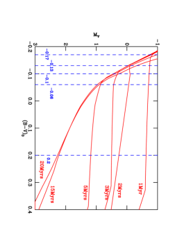
Figure 1: 1, 3, 5, 15 and 20 Myr isochrones from Siess et al. (2000) showing the MS, and pre-MS. $B-V$ colour cuts are shown for each age to isolate the MS. These are: -0.17, -0.1, -0.06 and 0.2 for 1, 3, 5, and older sequences respectively.

SFR	$B-V$	$E(B-V)$	$(B-V)_{0}$ Cut		Nominal age (Myr)	Data	Source	Size
	Cut		Data	Theory	Mayne et al. (2007)	type		(arcmins)
the ONC(1)	-	-	0.1	-0.13	1	$VI$ & $T_{eff}$	Hillenbrand (1997)	20
NGC6530(2)	0.5	0.32	0.18	-0.17	1	$UBVI$	Sung et al. (2000)	15
NGC2244(2)	0.45	0.47	-0.02	-0.13	$\approx 2^{(3)}$	$UBVI$$H_{\alpha}$	Park & Sung (2002)	15
NGC2264	-0.02	0.03	-0.05	-0.1	3	$UBVRI$	Mendoza V. & Gomez (1980)	30
NGC2362	0.04	0.09	-0.05	-0.1	3	$UBV$	Johnson & Morgan (1953)	30
$\lambda$ Ori	0.20	0.11	0.09	-0.1	3	$UBV$	Murdin & Penston (1977)	30
$\sigma$ Ori	0.03	0.06	-0.03	-0.06	4-5	$V_{T}B_{T}$(4)	Caballero (2007)	30
$\chi$ Per(7)	0.7	0.50	0.2	0.2	13	$UBV$	Slesnick et al. (2002)	2
h Per(7)	0.74	0.54	0.2	0.2	13	$UBV$	Slesnick et al. (2002)	2
NGC1960	0.25	0.20	0.05	0.2	16(5)	$UBV$	Johnson & Morgan (1953)	10
NGC2547	0.1	0.04	0.06	$>0.2$	38(6)	$UBV$	Claria (1982)	15

Table 1: The empirical and theoretical $B-V$ cuts for each SFR. The apparent cut has been converted into intrinsic colour using the $E(B-V)$ derived in Section 7. Also shown is the nominal age for each SFR from Mayne et al. (2007), the data type used and source for the data and initial memberships. The notes are as follows. (1) Individual extinctions derived from $T_{eff}$, see Section 5. (2) Individual extinctions derived using the Q-method (see Section 5.2). (3) Age from Park & Sung (2002). (4) Data in the $TYCHO$ photometric system. (5) Age from Sanner et al. (2000). (6) Age from Naylor & Jeffries (2006). (7) For h and $\chi$ Per stars have additionally been selected using apparent distance from the cluster centre (as defined in Mayne et al., 2007), selecting a circular area around the cluster centre of 2 arcmins in radius.

3 The models

In this work we have used the MS stellar interior models of the Padova (Girardi et al., 2002) and Geneva (Lejeune & Schaerer, 2001) groups. These provide an effective temperature ($T_{eff}$), luminosity and surface gravity. These values must then be converted into colours and magnitudes in the required photometric system (Johnson-Cousins) to allow the fitting of photometric data. Colours are found using a $T_{eff}$ to colour relation, and magnitudes using the bolometric correction to the luminosity. Both the colour-$T_{eff}$ relation and bolometric correction come from using the parameters from a stellar interior model to find the correct model atmosphere and then folding the resulting flux distribution through appropriate photometric filter responses. Once this is achieved the photometric colours and magnitudes must then be calibrated to a standard scale, using the colours of Vega in the photometric system. We have used three main isochrone and extinction systems calibrated to two different Vega colour systems, and we now detail each.

3.1 Geneva

The Geneva isochrones (as provided in Lejeune & Schaerer, 2001) are from the Geneva stellar interior models (basic set) in conjunction with the updated BaSeL-2.2 model atmospheres from Westera et al. (1999). To derive photometric magnitudes ($V$) they have adopted the bolometric corrections from Lejeune et al. (1998) which are defined to fit the empirical scale of Flower (1996) (not calibrated to the Sun). They calculate colours for Johnson-Cousins photometry using the filter response functions of Buser & Kurucz (1978) ($UBV$) and Bessell (1979) ($RI$). The colours and magnitudes of the isochrone are then calibrated to Vega colours of zero. For these isochrones we use the canonical extinction vectors, namely $E(U-B)/E(B-V)=0.73$, $A(V)/E(B-V)=3.1$ and $A(V)/E(V-I)=0.41$.

3.2 Geneva-Bessell

For the Geneva-Bessell isochrones we have used the interior models of Lejeune & Schaerer (2001), specifically their basic model set (“c”) generally applicable for stars with $M<12M_{\odot}$. Their conversion to photometric colours follows that of Bessell et al. (1998). Bessell et al. (1998) use the ATLAS9 atmosphere models of Castelli et al. (1997) (at solar metallicity only) and the filter responses of Bessell (1990) ($UBVRI$), to calculate the colour-$T_{eff}$ relations and bolometric corrections. The resulting Johnson-Cousins photometry is then calibrated to Vega colours of zero. In practice we carry out these conversions in our own code, since that allows us to also calibrate to what we term the non-zero system where $(B-V)_{Vega}=-0.002$ and $(U-B)_{Vega}=-0.004$.

3.3 Padova-Bessell

For the Padova-Bessell isochrones we use the stellar interior models of Girardi et al. (2002). The colours and magnitudes are then calculated using the conversions of Bessell et al. (1998) as for the Geneva-Bessell isochrones. The resulting Johnson-Cousins photometry is then calibrated to either Vega colours of zero or the non-zero system.

3.4 Extinction vectors in the Bessell system

It is well known that extinction vectors are actually a function of intrinsic colour (or spectral type). Bessell et al. (1998) provide extinction vectors as a function of colour based on the extinction curves of Mathis (1990). We therefore use these extinction vectors for the Geneva-Bessell and Padova-Bessell models.

The extinctions are provided for an $E(B-V)=0.3$. To check the range of extinctions to the SFRs studied here does not have a significant effect, we folded the solar abundance ATLAS 9 spectra with the “new” opacity distribution function (Castelli & Kurucz, 2004) through the bandpasses of Bessell et al. (1998). We then reddened the spectra according to the prescription of Cardelli et al. (1989) to yield an $E(B-V)$ of approximately 0.3. (This function is the one tabulated in the Mathis (1990) paper used by Bessell et al. (1998)). We used an $R_{v}$ of 3.2 since, when folded through the bandpasses of Bessell (1990) we found this gave the best match to the $BV$ extinction vector of Bessell et al. (1998). We calculated the difference in $A_{v}/E(B-V)$ for values of $E(B-V)$ of 1 (typical of the SFRs we have fitted) and 3 (approximating to the highest reddening of any SFR fitted). For $B-V<1.5$ we find the largest difference is -0.02 mags, which has a negligible impact on our fits.

3.5 $TYCHO$ photometry

For $\sigma$ Orionis the data were taken in the $TYCHO$ photometric system. We have fitted these data using the conversion of Bessell (2000) transform our Geneva-Bessell isochrones into the $TYCHO$ system. We have defined extinction vectors in the $TYCHO$ photometric system, in a process similar to that described in Section 3.4. We set our zero-points by requiring we reproduced the $T_{eff}$ vs $B-V$ relationship of Bessell (1990) and the $B-V$ vs $\Delta(B-V)$ relationship of Bessell (2000). This gave, for $(B-V)_{T}<0.065$

$${{(A_{V})_{T}}\over{E(B-V)_{T}}}=3.358+0.237(B-V)_{T},$$ (1)

and for $0.065<(B-V)_{T}<0.5$

$${{(A_{V})_{T}}\over{E(B-V)_{T}}}=3.387-0.207(B-V)_{T}.$$ (2)

These fits never deviate from the calculated curve by more than about 0.01 mags. At $B-V$=0 the $BV$ curves match to within 0.01 mags, though this worsens to 0.05 mags at $B-V$=1.

4 The fitting method

Throughout this example and later sections all the isochrone fits displayed and tests undertaken use the Geneva-Bessell Vega-zero isochrones. These isochrones are also adopted in Section 7 where we draw implications from the resulting distances and age ordering. As shown in Section 6 the model dependency between the different isochrones is practically very small.

4.1 Example fit: $\chi$ Per

It is most instructive to describe the fitting method via an example. Here we use the cluster $\chi$ Per which is approximately 13 Myrs old (Mayne et al., 2007), at a distance modulus of $11.85$ (Slesnick et al., 2002) with an $A_{V}\approx 1.6$ (Mayne et al., 2007) (the extinction is reasonably uniform). First, we describe the derivation of distance. Deriving a distance does require a known extinction, the derivation of which is described later in this section.

4.1.1 Fitting statistic, distance derivation

The fitting statistic used in this work is $\tau^{2}$, which is introduced in Naylor & Jeffries (2006). Fitting of MS data using this technique is described in Jeffries et al. (2007). $\tau^{2}$ is essentially a generalised $\chi^{2}$ statistic including uncertainties in two dimensions, and models with a two-dimensional distribution as opposed to a single isochronal line. The best fitting model is found by minimising $\tau^{2}$.

Once we have selected an isochrone we use a Monte-Carlo method to generate a colour-magnitude probability grid. Each pixel in this grid is assigned a value that gives the probability of finding a star drawn from the population represented by the isochrone, at any given colour and magnitude. The model is then adjusted through a range of distances and the values of $\tau^{2}$ for each star summed to calculate a total value of $\tau^{2}$ for each distance step, as detailed in Naylor & Jeffries (2006). These $\tau^{2}$ contributions were clipped, i.e. the contribution to the total $\tau^{2}$ for any single data point value is capped at some set value. Clipping avoids erroneously included non-members or anomalous objects many $\sigma$ from a given model overwhelming the result. The lowest total $\tau^{2}$ was then selected as the best fitting model.

Once a given fit was completed a probability of obtaining the resulting $\tau^{2}$, $P_{r}(\tau^{2})$, was calculated. If $P_{r}(\tau^{2})$ is far from 50%, the fitting is repeated with an additional systematic uncertainty added to the data. This is analogous to enlarging error bars to achieve a $\chi^{2}_{\nu}=1$. This process ensures the model is a good fit to the data and we are then able to derive the parameter uncertainties. To derive these uncertainties, we used the bootstrap method described in Naylor & Jeffries (2006), repeating the fitting 100 times and deriving 68% confidence intervals.

The resulting fit for $\chi$ Per is shown in Figure 2. The derived distance modulus and 68% confidence interval is $11.79<11.83<11.88$. This agrees with the most recent literature derivation of $11.85\pm 0.05$ from Slesnick et al. (2002), which was the same dataset.

Figure 2 and all subsequent figures showing fitted data have several elements requiring explanation. The shaded area shows the probability density of finding a star at a particular colour and magnitude (or colour and colour for extinction fitting). This density, $\rho$ is that from Equation 1 of Naylor & Jeffries (2006) generated for a specific isochrone, in this case Geneva-Bessell. The circles show the positions of the photometry and the bars give the uncertainties in magnitude and colour. For all the figures showing fitted data (except those using individual extinctions, see Section 5) the models have been adjusted to the natural space of the data i.e. apparent colour and magnitude.

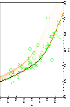
Figure 2: The distance fit for $\chi$ Per to the Geneva-Bessell isochrones. See Section 4.1 for details of the symbols.

4.1.2 Mean extinction fitting

To allow us to derive a distance, an extinction is required and is indeed crucial as changing it will change the distance derived for the stars we are fitting. We can derive a mean extinction by fitting the data to an isochrone in a colour-colour diagram. Where we have $UBV$ photometry we have simply fitted the sequence in $U-B$ vs $B-V$ in a similar fashion as that for a distance. However, instead of changing the distance, we evaluate $\tau^{2}$ at different values of the reddening. The resulting fit can be seen in Figure 3, with a best fitting $E(B-V)=0.50$. Figure 3 and all the subsequent figures showing extinction fitting contain the same components as those for distance fitting.

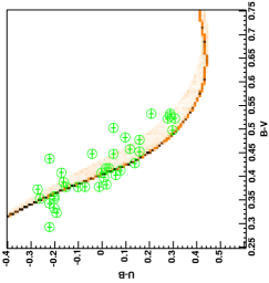
Figure 3: Figure showing $E(B-V)$ fit of $\chi$ Per to the Geneva-Bessell isochrones. See Section 4.1.2 for details of the symbols. Here a systematic shift in $E(B-V)$ as a function of colour ($U-B$) is evident, as in Figure 9. This is probably due to a difference in the photometric systems of Bessell et al. (1998) and Slesnick et al. (2002) (see Section 5.2).

In general fitting for an extinction using the $\tau^{2}$ method is desirable as photometric individual extinction methods rely on the star being a sinlge star or an equal mass-mass binary (see in Section 5.2). However, in some cases the dispersion in an $E(B-V)$ fit is too large, i.e. the scatter around the isochrone in the $U-B$ vs $B-V$ is too large to confidently assign one mean extinction. This is the case where there is significantly variable reddening across a SFR. Here we are forced to derive reddenings and therefore extinctions for each star from $UBV$ photometry alone using the Q-method (Johnson & Morgan, 1953). This is the case for NGC6530, NGC2244 and $\lambda$ Orionis. In addition in the case of the ONC $UBV$ colours are not available, here alternative methods must be used to derive extinctions. All these individual extinction derivations are detailed in Section 5.

4.2 Practical effect of assumptions

During fitting we have made three main assumptions about the MS and it is important to examine the validity of these. Firstly we have used an isochrone at an assumed nominal age which could be inaccurate for a given SFR. This may be important both just prior to turn-off and at the turn-on. Secondly, by using MS isochrones we have implicitly assumed that none of the stars fitted are on the pre-MS. Lastly, we have used isochrones of approximately solar composition ($Z=0.02$).

4.2.1 Age assumption

As a (coeval) stellar population ages, stars of a decreasing mass turn-off from the MS. In addition, stars close to but nominally below the turn-off age also move slightly red-wards in position in a CMD. As we remove stars brighter than the turn-off (Section 2.1) we avoid the age dependency of this feature, but we still retain the age dependency of the upper-MS. This shift of the upper-MS is small and furthermore in principle is modeled as we use a MS at the nominal age. However it is important to quantify this effect to ensure our distances are robust against assuming an incorrect age.

To test this upper-MS age dependency we have simulated photometry of a population based on a 1Myr Geneva-Bessell isochrone. We have then fitted these data (as described in Section 4.1) across a typical colour range, specifically blue-ward of $(B-V)_{0}=0.2$ (as shown in Table 1 cuts in all our SFRs are blue-ward of this), to a 10Myr Geneva-Bessell isochrone. This provides a measure of any extra uncertainty one accrues if the age assumption is incorrect. The resulting distance modulus and reddening are $dm\approx 0.001$ and $E(B-V)\approx-0.028$, for this factor ten in age. The effect of assuming an incorrect age on a derived distance and $E(B-V)$ is therefore negligible even for a large error in assumed age.

4.2.2 MS isochrones for a possible PMS population

As pre-MS stars approach the MS, just prior to the onset of hydrogen burning they enter a quasi-equilibrium state as hydrogen ignition starts. This delays their arrival onto the MS. The rate at which this phase progresses is a function of stellar mass and is, over the mass range of interest, very short in comparison to the evolution of the pre-MS. However, as such stars are slightly brighter than MS magnitudes, the distances derived may be systematically reduced as a function of age.

Some stars in our selected sequence may still be in this pre-MS phase even though appearing to be on the MS. This effect is greatest for the younger SFRs. However within the colour cuts we have used the deviation from the MS is a maximum of $\approx 0.05$ mag (in magnitude) and only affects a limited number of stars. Thus its overall effect will be much smaller than 0.05 mags.

4.2.3 Composition

As compositions are not available for all the SFRs studied we have assumed solar metallicity ($Z=0.02$). However there is evidence to suggest that some SFRs have a metallicity as low as half-solar (see Section 8.2.1). We must therefore quantify the possible effect varying composition could have on our relative distances. To do this we have again simulated a population, at 10Myr, using the Geneva isochrones with $Z=0.008$ (the closest match in the library to half-solar) and fitted these data for extinction and distance with solar composition isochrones (as described in Section 4.1). The resulting differences are, for reddening $E(B-V)=0.005$ and for distance modulus, $dm\approx 0.41$. This is a negligible difference in reddening and therefore extinction but a significant error in distance modulus. We have also fitted $\chi$ Per using the half-solar metallicity isochrones. Here we must use the colours and photometric system provided with the Geneva isochrones as our Geneva-Bessell isochrones utilise atmospheres of solar metallicity. The resulting distance modulus is $11.32<11.36<11.41$ and a reddening of $E(B-V)=0.51$ (using uncertainties of 0.018 for a $P_{r}(\tau^{2})\approx 0.5$). This means that if the metallicity is indeed $Z\approx 0.01$ the distance modulus to $\chi$ Per is actually $\approx 0.5$ mags less, making the stars older. This could have a major effect on the distances and ages of star-forming regions. Therefore composition information is vital in the future for more accurate SFR parameters. A further discussion of this problem can be found in Section 8.

5 Individual extinctions

As stated in Section 4.1.2 it is sometimes not possible or desirable to derive a mean extinction using the $\tau^{2}$ fitting method. In this Section we detail the cases where individual extinctions have been derived. Source by source extinctions have been used for six SFRs, using two methods. In all of these cases the extinctions applied will change the relative positions of the stars in colour magnitude space, as opposed to applying a mean extinction where the entire dataset is simply translated (shifted). Therefore, in the case of individual extinctions these must be applied prior to fitting, and the resulting figures show the data and model in intrinsic colour and extinction free magnitude.

5.1 Effective temperatures

5.1.1 the ONC

For the ONC $UBV$ photometry is unavailable, so fitting for a mean extinction using the method detailed in Section 4.1.2 is not possible. However Hillenbrand (1997) provides $VI$ photometry an of the centre of the ONC. We have used these temperatures, assumed a surface gravity ($log(g)$) of 4.5 and interpolated to obtain intrinsic colours from the $T_{eff}$ relations in Bessell et al. (1998). This allows us to derive an $A_{V}$ from $E(V-I)$ using $A_{V}=((3.26+0.22(B-V)_{0})/(1.32+0.06(V-I)_{0}))\times E(V-I)$ (derived from the extinction vectors of Bessell et al., 1998) and therefore calculate an unredenned magnitude. These resulting magnitudes and colours can then be fitted to derive a distance as in Section 4.1. For the analysis in Section 7 of this paper we have fitted the data using the intrinsic $B-V$ values appropriate for the effective temperatures, but we have also fitted the $V-I$ data, the result of which can be found in Section 6.

5.1.2 h and $\chi$ Per

The check the veracity of this technique, we compared the distances it yields for h and $\chi$ Per, with those from Sections 4 and 6. We used the $T_{eff}$ data from Slesnick et al. (2002) to derive intrinsic colours. However, as the $T_{eff}$ information is only available for the hottest stars, the colour range for fitting is small. Practically this means the uncertainties are large, particularly towards greater distances, but the answers for both techniques are consistent. As a further test, we have supplemented the objects with $T_{eff}$ data, with stars from the main catalogue dereddened to intrinsic colours using the mean extinction from the $\tau^{2}$ fitting. All the two techniques give consistent distances (Table 5), but those using the combined photometric and $T_{eff}$ datasets are more precise (ranges of 0.01 and 0.04 mags for h and $\chi$ Per respectively). This confirms that the $T_{eff}$ technique gives consistent answers, but we are wary of adopting the more precise technique for the remainder of this paper since our primary aim is to derive distances for many SFRs using a single method.

5.2 Q-method

The Q-method is a widely used method to derive individual source-by-source reddenings and therefore extinctions using a $U-B$ vs $B-V$ colour-colour diagram. Johnson & Morgan (1953) model the MS as the straight line in Figure 4. As this Figure shows, this can result in errors in the derived $A_{V}$ of up to 0.1 mag, to which must be added further 0.08 mag due to using colour independent extinction vectors. These are not intrinsic failings of the method, fitting a straight line to a modern isochrone, and using colour-dependent extinction vectors yields

$$Q=0.24(B-V)^{2}+3.257(B-V)+0.015,$$ (3)

in the Bessell et al. (1998) system. Within the ranges of colour in Table 2, this only differs by $<0.005$ mag from interpolating onto the isochrone. However in our “revised Q-method” we derive reddenings using isochone interpolation.

Age	$U-B$	$B-V$
1	$-0.17<U-B<-1.15$	$-0.06<B-V<-0.30$
3	$-0.17<U-B<-1.12$	$-0.06<B-V<-0.29$
5	$-0.17<U-B<-1.08$	$-0.06<B-V<-0.28$
15	$-0.17<U-B<-0.90$	$-0.06<B-V<-0.23$
30	$-0.17<U-B<-0.72$	$-0.06<B-V<-0.22$

Table 2: The approximate validity range for Equation 3 (not including multiple valued solutions) for several ages derived from the Geneva-Bessell isochrones, defined as regions where the real isochrone moves more than 0.01 in colour away from the straight line model.

Implicit in using a model, are assumptions as to the age and metallicity of the isochrone. We have tested the effect of both of these, and provided one remains within the colour ranges given in Table 2, their effect on the derived $A_{V}$ is less than $0.005$ mags. The blue limit in Table 2 corresponds to the turn-off, the red limit to approximately $U-B=B-V=0$. A further possible concern is shown in Figure 4; once the intrinsic colour is redward of $U-B\approx$-0.2, there is the possibility that the star actually lies on a redder part of the isochrone, leading to an ambiguity in the extinction. However, if the object is on the wrong part of the isochrone, the extinction is clearly anomalous, provided that the scatter in extinctions between stars is small.

The major concern when calculating individual reddenings and therefore extinctions using a colour-colour diagram is the effect of binarity. Figure 4 shows the range of colours occupied by unequal-mass binaries. In the absence of multiplicity information, any colour-colour method must dereden stars onto the single star/equal-mass binary sequence (see Section 4.1.2). As can be seen in Figure 3, without multiplicity information it is unclear whether a star should lie on the single star/equal-mass binary sequence or in the region occupied by unequal-mass binaries. The effect and range of this problem is shown in Figure 4. The outer binary envelope has been modeled and the possible differences in derived $A_{V}$ found. Figure 4 shows that binarity has an effect of up to $\Delta A_{V}\approx 0.15$ on the derived extinction. This effect becomes increasingly significant as one moves down (redder in $U-B$) the MS isochrone.

As the revised Q-method does not account for the scatter binaries produce in a CMD, or colour-colour diagram, it is a statistically ill-defined process. Effectively most of the intrinsic scatter from the binary sequence and photometric uncertainties is removed, in addition to that caused by variable extinction. Therefore, only when there is good evidence, from the mean extinction fitting method, that the extinction in a SFR is large and variable do we apply the revised Q-method. Thus we formulate the null hypothesis that the reddening or extinction is uniform. We fit to derive a mean extinction and subsequently a distance. These results can be found in Table 6 and are discussed in Section 6. However, in some cases of distance fitting, after applying a mean extinction, the addition of large systematic uncertainties was required to return a $Pr(\tau^{2})\approx 50\%$. In these cases we are forced to reject the null hypothesis and use the revised Q-method to derive individual extinctions. We believe that additional systematic uncertainties of up to 2% are credible, therefore we apply the revised Q-method in cases where our added systematic uncertainties exceed this level.

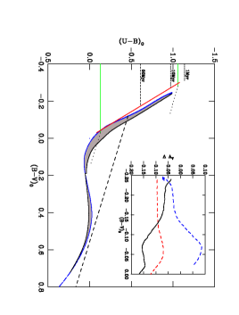
Figure 4: Geneva-Bessell 10 Myr isochrone including binaries (gray region enclosed by black line) and the Q-method MS straight line (red line). The horizontal dashed lines are the points at which the Geneva-Bessell isochrones evolve away from the MS. The horizontal bold lines are the validity region of the original Q-method. The two angled dotted lines are the extinction vectors at each end of the Q-method validity range from Bessell et al. (1998). Finally the large dashed line shows the region below which the solution for a given star can be multi-valued. The inset shows the differences in derived extinction ($\Delta A_{V}$). The top dashed line shows $\Delta A_{V}$ in the sense of the revised Q-method minus the old Q-method. The lower dashed shows $\Delta A_{V}$ derived from the reddest binaries minus the old Q-method. The bold line is $\Delta A_{V}$ derived from the reddest binaries minus the single star sequence.

5.3 SFRs with significantly variable reddening

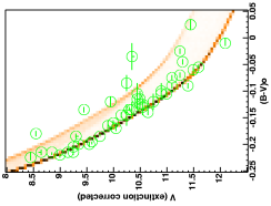
Figure 20: NGC6530 distance fit using Q-method extinctions (see Section 5.2). Figure shown in intrinsic colour and extinction corrected magnitude (see Section 5).

In Figure 6 we show the $\tau^{2}$ mean extinction fit for NGC6530. There is clearly a large scatter, which is also reflected in the corresponding distance fit, Figure 5. This scatter improves significantly when we use the revised Q-method, as shown in Figure 20. In addition the uncertainties in distance are significantly smaller when using the revised Q-method. The same arguments apply for NGC2244 and $\lambda$ Ori, and in Section 7 all three clusters are fitted using extinctions from the revised Q-method. For completeness the parameters derived for these three clusters using both methods are presented in Section 6. The resulting distance moduli derived using a mean extinction or the revised Q-method are consistent within the uncertainties.

We also attempted to use the revised Q-method for h Per, as it satisfied our criteria for non-uniform redenning. However, we found the $E(B-V)$ to vary systematically as a function of colour. This systematic shift in extinction with colour is evident in Figure 9. It shows that to fit the hotter stars and cooler stars simultaneously would require a change in the gradient of the isochrone. The same trend is observed for $\chi$ Per in Figure 3. Therefore, we attribute this behaviour to differences between the photometric systems of Slesnick et al. (2002) and Bessell et al. (1998). Moreover, as this systematic shift in $E(B-V)$ is not present in $V$ vs $B-V$ fit (see Figure 2) we further constrain the problem to a difference dominated by the $U$ band.

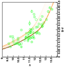
Figure 5: NGC6530 distance fit using mean extinction, the fit for which is shown as Figure 6.

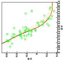
Figure 6: NGC6530 $E(B-V)$ fit.

6 Model dependency

Our results for all models are given in Tables 3-7. The fits have been optimised by adjusting the systematic uncertainties in colour and magnitude such that the $Pr(\tau)\approx 50\%$ (actually 44%-66%). The values for the reddening, the distance modulus with 68% confidence limits and, the added systematic uncertainties are shown. Table 3 shows the distances derived for $\sigma$ Orionis after conversion to the $TYCHO$ photometric system of Bessell (2000). Tables 4 and 5 contain the results fitting using a direct conversion from $T_{eff}$ to colour. The distances derived for each SFR using the mean extinction and revised Q-method for each set of isochrones are shown in Tables 6 and 7.

These results allow us to perform a brief comparison of the isochrones we have used, although not the main aim of this paper, it may aid the reader in adopting a particular result for a SFR of interest. Figure 7 shows the derived distances and associated uncertainties (68% confidence intervals) for each SFR and each set of isochrones, where a mean extinction has been derived. Figure 7 shows that for any given SFR the scatter between models is smaller than the uncertainties from the data. However, one could argue for a systematic shift of $\approx 0.05$ in distance modulus depending on the choice of Vega zero point.

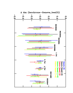
Figure 7: The distances and uncertainties (68% confidence intervals) derived for all SFRs and all isochrones, where a mean extinction has been derived. The results shown for each cluster are for, from left to right, Geneva (0) (blue), Geneva Bessell (0) (black), Padova Bessell (0) (red), Geneva Bessell (/=0) (green) and Padova Bessell (/=0) (yellow). All the resulting distances agree within the uncertainties for all models.

$TYCHO$ photometry
SFR	$\sigma$ Ori
Model (Vega cal)	dm	$\Delta$dm	Unc
Geneva-Bessell(0)	$7.84<7.94<8.10$	0.26	0.00
Padova-Bessell(0)	$7.72<7.93<8.03$	0.31	0.00
Geneva-Bessell($/=0$)	$7.79<7.94<8.07$	0.28	0.005
Padova-Bessell($/=0$)	$7.72<7.93<7.98$	0.26	0.005

Table 3: The distance moduli derived for $\sigma$ Ori in the $TYCHO$ photometric system for the different models, and calibrations to Vega colours of zero or Vega $B-V=-0.002$ and $U-B=-0.004$. Uncertainties required to achieve $0.40<P_{r}(\tau^{2})<0.60$ are also shown.

Intrinsic colours from $T_{eff}$
SFR	The ONC
Model (colour used)	dm	$\Delta$dm	Unc
Geneva-Bessell($B-V$)	$7.91<7.96<8.03$	0.12	0.010
Geneva-Bessell($V-I$)	$7.88<7.96<8.00$	0.12	0.013

Table 4: The distance moduli derived for the ONC using intrinsic colours derived from $T_{e}ff$ values of Hillenbrand (1997) in different colour indices. Uncertainties required to achieve $0.40<P_{r}(\tau^{2})<0.60$ are also shown.

Intrinsic colours from $T_{eff}$, $B-V$
SFR	$\chi$ Per			h Per
Model (stars used)	dm	$\Delta$dm	Unc	dm	$\Delta$dm	Unc
Geneva-Bessell(Hot)	$11.70<11.78<11.93$	0.23	0.003	$11.76<11.78<11.94$	0.18	0.004
Geneva-Bessell(Hot and cool)	$11.83<11.84<11.87$	0.04	0.00	$11.83<11.83<11.84$	0.01	0.019

Table 5: The distance moduli derived for h and $\chi$ Per using intrinsic colours derived from $T_{e}ff$ values of Slesnick et al. (2002) alone, or supplemented by cooler stars dereddened using an average extinction. Uncertainties required to achieve $0.40<P_{r}(\tau^{2})<0.60$ are also shown.

Reddening from $UBV$ fitting
SFR	NGC6530				NGC2244				NGC2264
Model (Vega cal)	dm	$\Delta$dm	Unc	$E_{(B-V)}$	dm	$\Delta$dm	Unc	$E_{(B-V)}$	dm	$\Delta$dm	Unc	$E_{(B-V)}$
Geneva(0)	$10.29<10.38<10.48$	0.19	0.0330	0.35	$10.62<10.78<10.94$	0.32	0.0470	0.47	$9.15<9.40<9.53$	0.38	0.018	0.06
Geneva-Bessell(0)	$10.16<10.34<10.43$	0.27	0.0305	0.32	$10.68<10.89<11.09$	0.41	0.0450	0.46	$9.26<9.37<9.52$	0.26	0.0160	0.04
Padova-Bessell(0)	$10.15<10.35<10.46$	0.31	0.0308	0.32	$10.73<10.81<11.00$	0.27	0.0450	0.45	$9.27<9.34<9.51$	0.24	0.0140	0.04
Geneva-Bessell($/=0$)	$10.25<10.27<10.34$	0.09	0.0330	0.32	$10.54<10.78<10.94$	0.40	0.0400	0.46	$9.18<9.39<9.51$	0.33	0.0160	0.04
Padova-Bessell($/=0$)	$10.26<10.28<10.32$	0.08	0.0330	0.32	$10.50<10.74<10.90$	0.40	0.0400	0.45	$9.18<9.40<9.50$	0.32	0.0160	0.04
SFR	NGC2362				$\lambda$ Ori				h Per
Model (Vega cal)	dm	$\Delta$dm	Unc	$E_{(B-V)}$	dm	$\Delta$dm	Unc	$E_{(B-V)}$	dm	$\Delta$dm	Unc	$E_{(B-V)}$
Geneva(0)	$10.48<10.58<10.69$	0.21	0.0150	0.12	$7.77<7.87<8.03$	0.26	0.022	0.12	$11.77<11.78<11.85$	0.08	0.0250	0.57
Geneva-Bessell(0)	$10.51<10.67<10.70$	0.19	0.0130	0.10	$7.89<7.98<8.16$	0.27	0.025	0.11	$11.77<11.78<11.84$	0.07	0.0260	0.54
Padova-Bessell(0)	$10.47<10.66<10.77$	0.30	0.0120	0.10	$7.81<7.98<8.15$	0.34	0.026	0.11	$11.63<11.65<11.74$	0.11	0.0310	0.52
Geneva-Bessell($/=0$)	$10.49<10.57<10.70$	0.21	0.0120	0.10	$7.86<7.96<8.13$	0.27	0.024	0.11	$11.76<11.78<11.80$	0.04	0.0270	0.54
Padova-Bessell($/=0$)	$10.47<10.55<10.72$	0.25	0.0120	0.10	$7.79<7.92<7.99$	0.20	0.025	0.11	$11.67<11.74<11.75$	0.08	0.0300	0.52
SFR	$\chi$ Per				NGC1960				NGC2547
Model (Vega cal)	dm	$\Delta$dm	Unc	$E_{(B-V)}$	dm	$\Delta$dm	Unc	$E_{(B-V)}$	dm	$\Delta$dm	Unc	$E_{(B-V)}$
Geneva(0)	$11.82<11.82<11.85$	0.03	0.010	0.52	$10.21<10.22<10.30$	0.09	0.0170	0.22	$7.85<7.93<7.97$	0.12	0.012	0.053
Geneva-Bessell(0)	$11.79<11.82<11.88$	0.09	0.005	0.50	$10.27<10.35<10.46$	0.19	0.0164	0.20	$7.98<8.05<8.09$	0.11	0.018	0.038
Padova-Bessell(0)	$11.77<11.79<11.86$	0.09	0.012	0.50	$10.17<10.29<10.43$	0.26	0.0164	0.20	$7.97<8.04<8.06$	0.09	0.018	0.038
Geneva-Bessell($/=0$)	$11.80<11.82<11.85$	0.05	0.011	0.50	$10.21<10.23<10.31$	0.10	0.0164	0.20	$7.92<8.03<8.07$	0.15	0.020	0.034
Padova-Bessell($/=0$)	$11.79<11.80<11.82$	0.03	0.010	0.50	$10.20<10.31<10.40$	0.20	0.0164	0.20	$7.92<7.99<8.05$	0.13	0.020	0.034

Table 6: The distance moduli and $E(B-V)$ values , derived using $U-B$ $B-V$ fitting, for each SFR using the different models and calibrations to Vega colours of zero or Vega $B-V=-0.002$ and $U-B=-0.004$. Uncertainties required to achieve $0.40<P_{r}(\tau^{2})<0.60$ are also shown.

Revised Q-method
SFR	NGC6530				NGC2244				$\lambda$ Ori
Model (Vega cal)	dm	$\Delta$dm	Unc	$\overline{E_{(B-V)}}$	dm	$\Delta$dm	Unc	$\overline{E_{(B-V)}}$	dm	$\Delta$dm	Unc	$\overline{E_{(B-V)}}$
Geneva-Bessell(0)	$10.49<10.50<10.60$	0.11	0.011	0.33	$10.66<10.77<10.81$	0.15	0.01	0.44	$7.99<8.01<8.12$	0.13	0.005	0.10
Padova-Bessell(0)	$10.47<10.48<10.58$	0.11	0.011	0.35	$10.68<10.76<10.84$	0.16	0.013	0.45	$7.93<8.01<8.09$	0.16	0.007	0.10
Geneva-Bessell($/=0$)	$10.36<10.41<10.49$	0.13	0.011	0.34	$10.67<10.76<10.89$	0.22	0.014	0.42	$7.95<7.97<8.11$	0.16	0.007	0.17
Padova-Bessell($/=0$)	$10.48<10.52<10.57$	0.09	0.009	0.34	$10.70<10.81<10.92$	0.22	0.013	0.43	$7.94<7.97<8.08$	0.14	0.007	0.12

Table 7: The distance moduli and mean $E(B-V)$ values, after application of Q, for each SFR using the different models, and calibrations to Vega colours of zero or Vega $B-V=-0.002$ and $U-B=-0.004$. Uncertainties required to achieve $0.40<P_{r}(\tau^{2})<0.60$ are also shown.

These results show that any model dependency in the extinctions and distances derived is small. A final statistical justification can be found from the results in Section 6. Here the systematic uncertainties required to achieve a $\tau^{2}$ of approximately one do not significantly favour any particular model.

7 Results

To simplify our discussion of the implications of our derived distances, we have adopted the results from the Geneva-Bessell isochrones. We display the resulting fits as Figures 2, 3 and 8-17. In Table 8 we provide a comparison of the adopted distances with 68% confidence intervals, with the distances assumed in Mayne et al. (2007). The best fitting $E(B-V)$ is also provided.

SFR	Mayne et al. (2007)		This work		$\Delta\overline{dm}$	$\Delta$ range	$E(B-V)$
	dm	Range	dm	range
the ONC	$8.01<8.38<8.75$	0.76	$7.91<7.96<8.03$	0.12	-0.42	-0.64	$\approx 0.40$(1)
NGC6530	10.48(4)	$\approx 0.40$(4)	$10.15<10.34<10.44$(2)	0.29	-0.14	-0.11	0.32
NGC6530	10.48(4)	$\approx 0.40$(4)	$10.49<10.50<10.60$(5)	0.11	+0.02	-0.29	0.33(5)
NGC2244	$10.55<10.72<10.87$(3)	0.33	$10.68<10.89<10.94$(2)	0.26	+0.17	-0.07	0.46
NGC2244	$10.55<10.72<10.87$(3)	0.33	$10.66<10.77<10.81$(5)	0.15	+0.05	-0.18	0.44(5)
NGC2264	9.6(6)	$\approx 0.40$(4)	$9.26<9.37<9.52$	0.26	-0.23	-0.14	0.04
NGC2362	$10.84<10.87<10.90$	0.06	$10.51<10.67<10.70$	0.19	-0.20	+0.13	0.10
$\lambda$ Ori	$7.73<7.90<8.07$	0.34	$7.99<8.01<8.12$(5)	0.13	+0.11	-0.21	0.10(5)
$\lambda$ Ori	$7.73<7.90<8.07$	0.34	$7.89<7.98<8.16$(2)	0.27	+0.08	-0.07	0.11
$\sigma$ Ori	$7.41<7.80<8.19$	0.78	$7.84<7.94<8.10$	0.26	+0.14	-0.52	0.06(7)
$\chi$ Per	$11.69<11.70<11.71$	0.20	$11.79<11.82<11.88$	0.09	+0.12	-0.11	0.50
h Per	$11.69<11.70<11.71$(8)	0.20	$11.77<11.78<11.84$	0.07	+0.08	-0.13	0.54
NGC1960	$10.40<10.60<10.80$(9)	0.40	$10.27<10.35<10.46$	0.19	-0.25	-0.21	0.20
NGC2547	$7.92<8.18<8.47$(10)	0.54	$7.98<8.05<8.09$	0.11	-0.13	-0.43	0.038

Table 8: Distance moduli and range assumed in Mayne et al. (2007) and those derived in this work. Notes are as follows. (1) Individual extinctions from $T_{eff}$, value given is approximate mean. (2) Distance derived using mean extinction derivation from $\tau^{2}$ fitting. (3) Not included in Mayne et al. (2007), distance from Hensberge et al. (2000). (4) Typical uncertainties assumed as none were provided in literature source. (5) Resulting distance after application of extinctions derived using Q-method (see Section 5.2). A mean extinction is quoted. (6) Typical uncertainties assumed as literature distance is the mean of many values. (7) $E(B-V)$ from Brown et al. (1994). (8) Assumed to be at the same distance as $\chi$ Per in Mayne et al. (2007). (9) Not included in Mayne et al. (2007), distance from Park & Sung (2002). (10) Not included in Mayne et al. (2007), distance from Robichon et al. (1999).

7.1 Notes on results

We would have liked to include the sub-group CepOB3b in this paper, but after application of the Q-method the resulting colour range for the stars available for fitting was prohibitively low for distance fitting. Literature derivations of extinction (Garrison, 1970; Blaauw et al., 1959) rely on intrinsic colours derived from other isochrones so cannot be used to fit with the Geneva-Bessell isochrones.

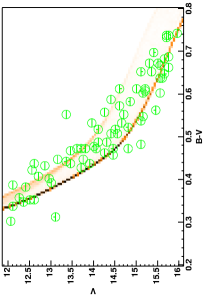
Figure 8: h Per distance fit.

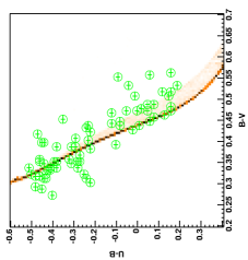
Figure 9: h Per $E(B-V)$ fit. Here a systematic shift in $E(B-V)$ as a function of colour ($U-B$) is evident, as in Figure 3. This is probably due to a difference in the photometric systems of Bessell et al. (1998) and Slesnick et al. (2002) (see Section 5.2).

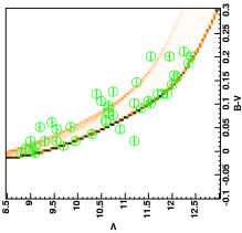
Figure 10: NGC1960 distance fit.

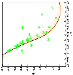
Figure 11: NGC1960 $E(B-V)$ fit.

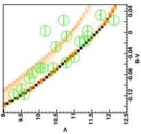
Figure 12: NGC2362 distance fit.

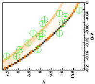
Figure 13: NGC2264 distance fit.

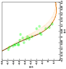
Figure 14: NGC2362 $E(B-V)$ fit.

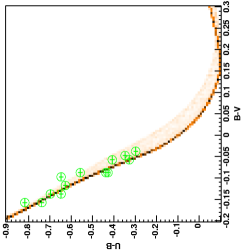
Figure 15: NGC2264 $E(B-V)$ fit.

Figure 16: NGC2547 distance fit.

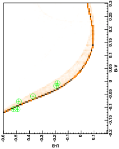
Figure 17: NGC2547 $E(B-V)$ fit.

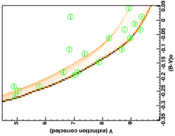
Figure 18: The ONC distance fit. Figure shown in intrinsic colour and extinction corrected magnitude (see Section 5).

Figure 19: $\sigma$ Orionis distance fit.

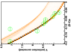
Figure 21: $\lambda$ Ori distance fit using the Q-method extinctions (see Section 5.2). Figure shown in intrinsic colour and extinction corrected magnitude (see Section 5).

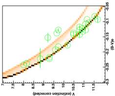
Figure 22: NGC2244 distance fit using Q-method extinctions (see Section 5.2). Figure shown in intrinsic colour and extinction corrected magnitude (see Section 5).

8 Implications

We have now derived a self-consistent set of distances (and extinctions) to, in general, a higher precision than that existing in the literature, with statistically meaningful uncertainties for these distances. We now discuss some of the key implications of both the individual distances and of the entire dataset.

8.1 Individual Distances

Of the SFRs studied in this work distances derivations for eight are of particular note. Here we have converted the distance moduli to a distance to allow more obvious comparisons.

8.1.1 The ONC

We have increased the precision of the distance estimate for the ONC by a factor of 7 compared to that used in Mayne et al. (2007). This new distance is also closer than the previously accepted result from the maser measurements of Genzel et al. (1981), by $0.42$ mag. Conversely this new distance, $391^{+12}_{-9}$ pc agrees superbly with several recent derivations in the literature. Firstly, Jeffries (2007a) finds a distance of $392\pm 32$ pc from the rotational properties of low-mass pre-MS stars (after removing accreting objects). Secondly, a parallactic distance of $389^{+24}_{-21}$ pc from very long baseline array observations has been found by Sandstrom et al. (2007). Lastly, Kraus et al. (2007) find a distance of $434\pm 12$ or $387\pm 11$ pc by modeling the orbit of the $\theta^{1}$Ori C binary system. They adopt 434 pc as the likely result after comparison to the distance obtained by Jeffries (2007a) for all objects including those showing evidence of accretion. Clearly, our result favours the solution yielding 387 pc. A convenient round number which agrees with the majority of the recent derivations is 400 pc.

This closer distance ($391^{+12}_{-9}$ pc compared to $480\pm 80$ pc) has important implications for the stellar population of the ONC. It means the pre-MS population lies $0.42$ mags fainter in absolute magnitude in the CMD. This will force the isochronal age of stars older, but perhaps more importantly increase their spread in isochronal age derived from a CMD (see the discussion in Palla et al., 2005). This is due to the bunching of older isochrones towards the zero-age-main-sequence (ZAMS). In fact there is also evidence of a spread in the CMD from the MS members we have used to derive a distance. As can be seen in Figure 23, MS stars exist at a position in the CMD suggesting isochronal ages of up to 10 Myrs, which is at variance with the median pre-MS age of $\approx 2$ Myr (after allowing for the revised distance). This is discussed further in Section 8.2.2.

Figure 23: The ONC with a Geneva-Bessell 1 Myr MS isochrone and the Pre-MS isochrones of Siess et al. (2000) for 1, 3 and 10 Myrs. Stars appear to lie at the turn-on for an age of 10 Myr.

8.1.2 $\sigma$ Orionis

We have improved the precision of the distance estimate used for $\sigma$ Orionis in Mayne et al. (2007) by a factor of 2. Caballero (2007) derives a distance based on $TYCHO$ photometry of $360^{+70}_{-60}$ pc. Although we also use the $TYCHO$ photometry, we use updated photometric conversions from Bessell (2000). We derive a distance of $389^{+34}_{-24}$ pc, a value more precise than, but in agreement with that of Caballero (2007).

8.1.3 NGC2547

For NGC2547 we have increased the precision in distance from that adopted in Mayne et al. (2007) by a factor of 5. In this work we derive a distance of $407^{+8}_{-13}$ pc, which compares favourably with the $HIPPARCOS$ result of $433^{+62}_{-49}$ pc from Robichon et al. (1999). However, Naylor & Jeffries (2006) use pre-MS isochrones to obtain a distance of $361^{+19}_{-8}$ pc. The age and distance derivation in Naylor & Jeffries (2006) is consistent with the Li depletion boundary, which is also based on pre-MS models. Therefore we conclude the difference in distance is attributable to a model-dependent difference between the MS and pre-MS models. Interestingly we also obtain a different reddening, $E(B-V)=0.038$ to that of Claria (1982), $E(B-V)=0.06\pm 0.02$ which is used in Naylor & Jeffries (2006). However, this does not have a significant impact on their distance, and so does not explain the discrepancy between the MS and pre-MS distances.

8.1.4 NGC2244

The distance to NGC2244 derived in this work is $1\,425^{+27}_{-70}$ pc, using individual extinctions from the revised Q-method (see Section 5.2). This compares well to the literature result of $1\,390\pm 100$ pc from eclipsing binaries of Hensberge et al. (2000). Previous MS isochrone fitting studies placed this SFR at $1\,667^{+128}_{-118}$ pc (Perez et al., 1987), and $1\,660$ pc (Park & Sung, 2002, we use the same data as this study). Our result confirms the closer distance of Hensberge et al. (2000) and is marginally consistent with the studies yielding a greater distance. The new distance will move the cluster pre-MS fainter or older by $\approx 0.3$ mags.

8.1.5 NGC2362

Our derived distance for NGC2362, $1\,361^{+19}_{-97}$ pc is closer and less precise than that used in Mayne et al. (2007). In Mayne et al. (2007) we adopted a distance of $1\,493^{+21}_{-20}$ pc, an incredibly precise value from Balona & Laney (1996), derived using a form of MS fitting to narrow band photometry. For the sake of a consistent relative experiment we adopt our new distance for subsequent analysis.

8.1.6 h and $\chi$ Per

The distance we have derived for $\chi$ Per of $2\,312^{+65}_{-32}$ pc agrees well with the recent literature result of $2\,344^{+55}_{-53}$ pc of Slesnick et al. (2002), as stated in Section 4.1. They employ spectroscopy as well as the Q-method (with what appears to be an updated MS line, but canonical reddening vectors) combined with MS isochrone fitting to derive this distance. Interestingly they also derive a spectroscopic parallax distance of $3\,162$ pc. This method involves dereddening stars with known spectral types onto an intrinsic MS; they conclude that recalibration of these intrinsic colours is required. Also Slesnick et al. (2002) find h and $\chi$ Per to be at approximately the same distance, agreeing with the majority of the literature (e.g Keller et al., 2001). Our distance derivation for h and $\chi$ Per are also consistent with both these clusters being at the same distance.

8.2 Global issues

In this section we discuss general implications related to the dataset as a whole.

8.2.1 Metallicity

There is little work on the metallicity of SFRs. James et al. (2006) show that the metallicity is solar or very slightly sub-solar for the majority of stars in the Lupus, Chamaeleon and CrA SFRs. Conversely recent eclipsing binary results suggest approximately half-solar metallicity for h and $\chi$ Per and Collinder 228 (Southworth et al., 2004, 2004a; Southworth & Clausen, 2007), and solar metallicity for NGC6871 (Southworth et al., 2004b, $Z=0.02$). If compositions do indeed vary as is suggested from the above results then distances derived to these SFRs must be re-derived after a comprehensive composition survey. As discussed in Section 4.2.3, adopting a half-solar composition for $\chi$ Per (for example) results in a fall of the derived distance modulus by $\approx 0.5$ mags. A similar result would apply for h Per. This would have a severe impact on any age ladder, and thus on any conclusions about secular evolution, such as disc lifetimes.

8.2.2 Age spreads and the R-C gap overlap

As can be seen in Table 1 the faint red edge of the MS defined using pre-MS isochrones and the edge of the apparent MS in the CMD do not agree for the younger SFRs. This means that there are MS stars which lie fainter and redder than the base of the MS predicted by theory. The models predict that, for a coeval population, the brightest stars still on the pre-MS (at the red edge of the R-C gap) are similar in magnitude to the faintest stars on the MS (which are at the blue edge of the R-C gap). This extension of the MS to magnitudes fainter than the head of the pre-MS we term the R-C gap overlap. The R-C gap overlap is most apparent in the younger SFRs. One of the best examples is shown in Figure 23; the faintest stars on the MS in the ONC must be at least 10 Myrs old to have reached the MS, whilst the median age of the pre-MS is around 2 Myrs. An apparent age spread can also be seen for NGC2264 in Figure 25 for both the MS and pre-MS populations.

This apparent extension (along a MS line) below the turn-on for almost all SFRs can be interpreted as an age spread within the SFR. This suggests that stars have evolved across the R-C gap before theory would predict for a coeval population and must therefore be older. This would explain why the R-C gap overlap is less apparent in the older SFRs. As the age of an isochrone increases they become fainter and move towards the ZAMS. Lower mass stars on the pre-MS contract more slowly as they age. Therefore, the same difference in age for an older population produces a smaller change in $V$ than for a younger population. Thus the R-C gap overlap for older SFRs is harder to detect.

Despite the R-C gap overlap being harder to detect in old SFRs, an isochronal age spread can still be seen in the HM stars. As shown for $\chi$ Per in Figure 24 stars again lie below the turn-on and above the apparent turn-off for the best fitting or literature age of 13 Myrs. If one assumes the age is incorrect and increases it to match the turn-on, the turn-off will move fainter and exacerbate the problem for the brighter stars. Photometric variability and errors, and binarity have been shown not to completely account for these isochronal age spreads for the pre-MS in Burningham et al. (2005) and cannot account for the R-C gap overlap.

Hypothesising such an age spread supports other results from isochrone modeling. It is well known that individual ages derived using pre-MS isochrone fitting also show an age spread (see for example Palla et al., 2005; Slesnick et al., 2004). Also, Jeffries (2007b) finds a direct spread in the radii (and hence by implication age) of the PMS stars in the ONC, at a given effective temperature, a method free from isochrone theory.

However it is dangerous to interpret the R-C gap overlap, or the spreads in stellar radii and isochronal age, as real age spreads. As shown in Tout et al. (1999) accretion can act to force a star bluer and temporally older. This shift in position within a CMD means an isochronal age spread derived from pre-MS fitting does not necessarily imply a real underlying age spread of the same magnitude. Additionally Siess et al. (1999) find that the evolution of an accreting star is accelerated, with the star having a smaller radius and therefore lower luminosity than a non-accreting coeval counterpart. This result shows that age spreads derived from spreads in radii or from the R-C gap overlap again do not necessarily imply a real spread in age.

Whether star formation is rapid ($\approx 1$ Myr) or slow ($\approx 5-10$ Myrs) is currently an active debate (e.g Krumholz & Tan, 2007; Ballesteros-Paredes & Hartmann, 2007). Not withstanding different star formation rates or several episodes of star formation, the age spread of the bulk of the population within an SFR is an approximate measure for the local star formation time. Apparent age spreads within a CMD are often used to support the model of slow star formation (Palla et al., 2005; Burningham et al., 2005; Jeffries, 2007b). In the rapid star formation model these spreads of apparent age are dominated by accretion effects, and the residual real age spread is small. If accretion does indeed act to scatter a star within the CMD and even artificially accelerate its evolution or contraction, isochronal ages should not be used to represent real age spreads. Moreover, isochronal ages (based on turn-ons, turn-offs or pre-MS fitting) for individual stars without a known accretion history do not represent the true age of the star and therefore should not be used to support evolutionary theories. Indeed, it is even hard to argue that a median or mean age for a given SFR derived from isochrone fitting has any real meaning. Perhaps, following the results in Siess et al. (1999) and Tout et al. (1999), if accretion causes a decrease in the star’s radius, therefore increasing its isochronal age, the most accurate representative age for a given cluster is that of the youngest stars having the lowest accretion histories. However, this would mean a dramatic change in the ages for most SFRs, for example the youngest stars in the ONC are $\approx 0.1$ Myrs (Hillenbrand, 1997) and many older SFRs still contain active star formation and embedded objects.

A useful indicator to quantify these perceived spreads may be the R-C gap overlap, where the minimum mass object to have developed a radiative core and to have joined the MS can be compared to the maximum mass stars still existing on the convective pre-MS. This overlap then provides a precise diagnostic for the apparent age spreads. Whether these spreads show a real age spread or are indicative of the range of accretion histories present depends on the model adopted.

Given the problems with SFR ages the best approach currently is to compare observations of two different SFRs. Either deriving an age order by assuming a similar range of accretion rates within each SFR, or by using the R-C gap overlap to derive approximate differences in the range of accretion rates. An example of this can be seen in Figure 25, showing the absolute magnitude and intrinsic colour for the stars of the ONC and NGC2264 (taken from Mayne et al., 2007, and sources referenced therein). The locus of the pre-MS in NGC2264 clearly lies slightly below that of the ONC, but the MS section is strikingly similar. In addition Figure 25 shows the MS for the SFRs extending below the predicted turn-on. Moreover the brightest MS stars in both populations are at similar magnitudes i.e. the turn-off is in a similar position with stars lying on the apparent MS above the turn-off (as seen in Figure 24). As the apparent MS and pre-MS in both clusters appear to extend to similar points, i.e. the R-C gap overlap is similar, suggesting a similar range of accretion histories or ages for each cluster. So, in conclusion, the MS and pre-MS sections imply a large isochronal age spread as seen in Figure 23, and deriving ages and age spreads from these sections of the sequence would lead to a similar result for the ONC and NGC2264. However, comparing the sequences as a whole show that NGC2264 is more evolved than the ONC.

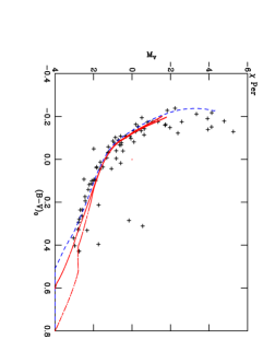
Figure 24: $\chi$ Per with a Geneva-Bessell 13 Myr MS isochrone (dashed line) and the pre-MS isochrones of Siess et al. (2000) for 13 and 23 Myrs (bold lines). Stars appear to lie below the turn-on and above the turn-off for an age of 13 Myr .

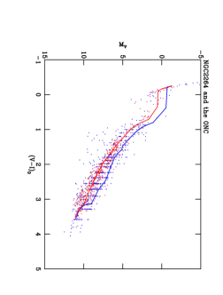
Figure 25: Absolute magnitude as a function of intrinsic colour for stars in the ONC and NGC2264 (taken from Mayne et al., 2007, and sources referenced therein) adjusted using the extinctions and distances from this work. The blue dots are the ONC and the red dots are NGC2264. The locus of points for NGC2264 can be seen to lie below the ONC, however the MS section is very similar in extent for each SFR, i.e. the turn-on appears coincident. The pre-MS isochrones from Siess et al. (2000) are shown for 1 and 3 Myrs. Most importantly in the MS section stars from both populations extend below the turn-ons whilst for both SFRs the peak of the MS (brightest stars) is similar i.e. the turn-offs do not appear significantly different, although this is based on only a few stars.

8.2.3 Secular evolution and ages

We now reconstruct the age ladder of Mayne et al. (2007) using the new distances and extinctions from Table 8. We have however changed the process slightly. Given that the new distances are generally more precise, we assume that the MS for each SFR will be approximately coincident in the CMD. Therefore, we plot the individual photometric points for this section of each sequence. Then for stars redward of the R-C gap we fit a spline through the median points. We retain the ZAMS subtracted space as a presentation tool (where the colour at each magnitude has the corresponding ZAMS colour subtracted from it as in Mayne et al., 2007). We are unable to include NGC2244 as the pre-MS of this SFR is not studied in Mayne et al. (2007). We do however, include in this section four SFRs from Mayne et al. (2007) not studied in this work, where we adopt literature distances and extinctions.

As the distance moduli for some SFRs have changed from those adopted in Mayne et al. (2007) the nominal ages may also have changed. The distance moduli which have changed by more than $0.2$ mag which were discussed in Mayne et al. (2007) are the ONC, NGC2264, NGC2362, $\lambda$ Ori and $\sigma$ Ori. In addition the relative distances and extinctions for h and $\chi$ Per have changed slightly, therefore we have refitted these clusters. Following Mayne et al. (2007) we have adjusted h Per to the distance and extinction of $\chi$ Per and combined the sequences prior to fitting them. We have included the entire sequence in a fit to h and $\chi$ Per providing an empirical ZAMS blue-ward of the R-C gap.

Following Mayne et al. (2007) we present fiducial empirical isochrones bounding the target empirical isochrone in a CMD of absolute magnitude and intrinsic colour and in ZAMS subtracted space. Figure 26 shows the pre-MS of NGC2264, after application of the distances in this work, lying only slightly below the ONC, the pre-MS of NGC2362 is shown to lie below these sequences. A combined h and $\chi$ Per empirical isochrone is also shown as a lower fiducial in Figures 26 and 27, with Figure 27 using NGC2264 as an upper fiducial. Figure 27 also shows the empirical isochrones for the pre-MS of both $\lambda$ Ori and $\sigma$ Ori, the former lying above NGC2264 and the latter below. From these two figures we can create an age ladder (youngest to oldest) and assign nominal ages: the ONC (2 Myrs), $\lambda$ Ori , NGC2264 and $\sigma$ Orionis (3 Myrs), NGC2362 (4-5 Myrs) and finally h and $\chi$ Per (13 Myrs).

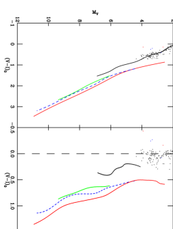
Figure 26: The MS stars (dots) and pre-MS empirical isochrones (continuous lines) of the ONC (red), h and $\chi$ Per (black) and NGC2362 (green), with the pre-MS empirical isochrone of NGC2264 (blue) as a dashed line. The left panel is a CMD of absolute magnitude and intrinsic colour with the right panel is in ZAMS subtracted space.

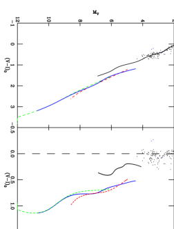
Figure 27: The MS stars (dots) and pre-MS empirical isochrones (continuous lines) of NGC2264 (blue) and h and $\chi$ Per (black), with the pre-MS empirical isochrones of $\lambda$ Ori (red) and $\sigma$ Ori (green) as dashed lines. The right panel shows the same in ZAMS subtracted space. The left panel is a CMD of absolute magnitude and intrinsic colour with the right panel is in ZAMS subtracted space.

We have repeated this method to obtain positions in an age ladder for each SFR for which we have enough data to create an empirical isochrone. This has resulted in the creation of a new group in addition to those of Mayne et al. (2007). This group, at a nominal age of 2 Myrs, contains the ONC and NGC6530, as it lies older than IC5146 but marginally younger than NGC2264. The resulting age groups from this work and those from Mayne et al. (2007), alongside literature estimates of the fraction of stars exhibiting infrared (IR) excess (i.e. candidates for an associated disc), are shown in Table 9. It is important to note that we have only updated distances for some of the SFRs.

SFR	Nominal age		Fraction of stars with IR excess
	This work	Mayne et al. (2007)
IC5146	-	1	-
NGC6530	2	1	$44\%$(7)
the ONC	2	1	$80\pm 5\%$(1)
$\lambda$ Ori	3	3	$\approx 25\%$,$\approx 14\%$,$\approx 31\%$(6)
CepOB3b	-	3	-
NGC2264	3	3	$52\pm 10\%$(1)
$\sigma$ Ori	3	4-5	$31.1\pm 3.8\%$, $26.6\pm 2.8\%$ and $33.9\pm 3.1\%$(2)
NGC2362	4-5	3	$12\pm 4\%$(1),$7\pm 2\%$(3)
IC348	-	4-5	$65\pm 8\%$(1)
NGC7160	-	10	$\approx 20\%$(4)
h and $\chi$ Per	13	13	$2-3\%$(8)
NGC1960	20	20	$3\pm 3\%$(1)
NGC2547	40	38	$\approx 7\%$(5)

Table 9: The new nominal ages of SFRs from this work and those from Mayne et al. (2007) are shown in addition to the fraction of stars with IR excesses. NGC2244 from this work was not studied in Mayne et al. (2007) so is omitted. IC5146, CepOB3b, IC348 and NGC7160 are studied in Mayne et al. (2007) and included here by adopting literature distances and extinctions. The notes are as follows. (1) Haisch et al. (2001). (2) Hernández et al. (2007). First value for TTS stars (approximate mass range $1-0.1M_{\odot}$). Second and third values for entire sample, first for thick discs and second for thick and evolved discs. (3) Dahm & Hillenbrand (2007). (4) Sicilia-Aguilar et al. (2005). (5) Young et al. (2004). (6) Barrado y Navascués et al. (2007). Firstl value derived from the IRAC CCD. Second and third from spectral-energy distribution (SED) fitting, thick discs then thin and thick discs combined. All values in the approximate mass range $0.1-1.0M_{\odot}$. (7) Prisinzano et al. (2007). (8) Currie et al. (2007), for h and $\chi$ Per stars fainter than J=13.5, stars brighter than this have $0\%$ disc fraction. It is important to note that each of these studies is over a different mass range (due to different distances and apparent magnitude ranges) and excess candidates were selected in a heterogeneous fashion.

The infrared excess fractions from Table 9 can be used to infer the presence of a disc, then by comparing the disc fraction across a range of SFRs one can examine the evolution of these discs, as in Haisch et al. (2001). Figure 28 shows the logarithmic nominal ages for the SFRs from Table 9 and the inferred fraction of stars with discs. However the disc fractions inferred from the data in Table 9 come from different mass ranges, dependent on the apparent magnitude range (and therefore distance) of the target SFR. Additionally, the excess criteria used are different, with studies such as Hernández et al. (2007) using the Spitzer Space Telescope IRAC and MIPS camera channels, whereas disc fractions in Haisch et al. (2001) were calculated using $JHKL$ excesses. Therefore, given the heterogeneous nature of these data one cannot draw strong conclusions from Figure 28 regarding the disc fraction as a function of age.

Despite its limitations, Figure 28 is not consistent with a uniform decay, revealing further possible evidence of environmental effects as suggested in Mayne et al. (2007). As an example we examine the inferred disc fractions of three SFRs in the same age group (nominal age of 3 Myrs); NGC2264, $\lambda$ Orionis and $\sigma$ Orionis, with distances of $dm=9.37$, $8.01$ and $7.94$ respectively. The disc fractions adopted are (in the same order) $52\pm 10\%$ (JHKL, Haisch et al., 2001, for masses greater than $0.85M_{\odot}$), $\approx 25\%$ (from IRAC data, Barrado y Navascués et al., 2007, all discs in spectral range of M0-M6.5 or approximate mass range of $0.1-0.8M_{\sun}$ using pre-MS isochrones), and $31.1\pm 3.8\%$ (from IRAC data, Hernández et al., 2007, all stars in the approximate mass range $0.1-1.0M_{\sun}$). In the case of these three SFRs NGC2264 has an inconsistent disc fraction, it is much higher than that of the other two SFRs. These disc fractions are taken from differing mass ranges and the SFRs are at different distances which could lead to sensitivity problems in the $L$ band as suggested for NGC2362 by Lyo et al. (2003). However, in this case the further distance to NGC2264 would result in fewer L band detections and the lower mass limit being higher is also likely to decrease the detected disc fraction. Therefore, it is likely that a consistent experiment would increase the discrepancy between NGC2264 and the two SFRs with lower disc fractions. However, even ignoring the particular case at a nominal age of 3 Myrs it is clear that the these data do not necessarily imply a smooth decline in disc fraction with age, suggesting other, presumably environmental factors may affect disc lifetimes.

Figure 28: Figure showing the log(nominal age) of each SFR with the IR excess from various literature sources. The inset panel shows the region 0-5 Myrs enlarged.

9 Conclusions

1. We have derived a self-consistent set of distances of generally higher precision than previously available for a set of SFRs in the age range 1-40 Myrs. We have also derived distances using several other models and calibrations (see Section 6).

2. In addition to these new distances and reddenings (or extinctions) we have reconstructed the age ladder of Mayne et al. (2007) assigning new nominal ages, as shown in Table 9. To enable the reader to add other SFRs to this ladder the pre-MS splines are freely available from the cluster collaboration home page, and the CDS archive.

3. We have shown that metallicity information is now vital for accurate relative distances to SFRs. This is especially true if one is attempting to characterise evolutionary indicators such as disc fractions as a function of age, or trying to uncover environmental effects (such as the effect of ionising winds from massive stars on planet formation from discs).

4. We have discussed that the overlapping region of the R-C gap could be used to derive spreads in isochronal age in a CMD, i.e. the apparent age difference between the maximum mass star still on the convective pre-MS and the minimum mass star which has reached the MS. If star formation is slow and isochronal ages of individual stars are reliable this would provide a direct measurement of the age spreads present in SFRs. If star formation is rapid the R-C gap overlap region reveals the underlying spread in accretion histories within an SFR. This is important as for rapid star formation, if an accretion history is unknown isochronal ages derived from a position in a CMD do not represent the true age of a star. Indeed it is therefore likely that if a rapid star formation model is accurate median or mean ages drawn from a population are also invalid. A more useful approach may be to compare SFRs using age ladder arguments or perhaps to use the age of the youngest stars which have the lowest accretion history.

5. We have shown further evidence for non-uniform decay of discs in SFRs, although new comparisons must be made using consistent disc fraction indicators and mass ranges.

References

- Ballesteros-Paredes & Hartmann (2007) Ballesteros-Paredes J., Hartmann L., 2007, Revista Mexicana de Astronomia y Astrofisica, 43, 123
- Balona & Laney (1996) Balona L. A., Laney C. D., 1996, MNRAS, 281, 1341
- Barrado y Navascués et al. (2007) Barrado y Navascués D., Stauffer J. R., Morales-Calderón M., Bayo A., Fazzio G., Megeath T., Allen L., Hartmann L. W., Calvet N., 2007, ApJ, 664, 481
- Bessell (1979) Bessell M. S., 1979, PASP, 91, 589
- Bessell (1990) Bessell M. S., 1990, PASP, 102, 1181
- Bessell (2000) Bessell M. S., 2000, PASP, 112, 961
- Bessell et al. (1998) Bessell M. S., Castelli F., Plez B., 1998, A&A, 333, 231
- Blaauw et al. (1959) Blaauw A., Hiltner W. A., Johnson H. L., 1959, ApJ, 130, 69
- Bonatto et al. (2004) Bonatto C., Bica E., Girardi L., 2004, A&A, 415, 571
- Brown et al. (1994) Brown A. G. A., de Geus E. J., de Zeeuw P. T., 1994, A&A, 289, 101
- Burningham et al. (2005) Burningham B., Naylor T., Littlefair S. P., Jeffries R. D., 2005, MNRAS, 363, 1389
- Buser & Kurucz (1978) Buser R., Kurucz R. L., 1978, A&A, 70, 555
- Caballero (2007) Caballero J. A., 2007, A&A, 466, 917
- Cardelli et al. (1989) Cardelli J. A., Clayton G. C., Mathis J. S., 1989, ApJ, 345, 245
- Castelli et al. (1997) Castelli F., Gratton R. G., Kurucz R. L., 1997, A&A, 318, 841
- Castelli & Kurucz (2004) Castelli F., Kurucz R. L., 2004, ArXiv Astrophysics e-prints
- Claria (1982) Claria J. J., 1982, A&AS, 47, 323
- Currie et al. (2007) Currie T., Balog Z., Kenyon S. J., Rieke G., Prato L., Young E. T., Muzerolle J., Clemens D. P., Buie M., Sarcia D., Grabu A., Tollestrup E. V., Taylor B., Dunham E., Mace G., 2007, ApJ, 659, 599
- Dahm & Hillenbrand (2007) Dahm S. E., Hillenbrand L. A., 2007, AJ, 133, 2072
- Flower (1996) Flower P. J., 1996, ApJ, 469, 355
- Garrison (1970) Garrison R. F., 1970, AJ, 75, 1001
- Genzel et al. (1981) Genzel R., Reid M. J., Moran J. M., Downes D., 1981, ApJ, 244, 884
- Girardi et al. (2002) Girardi L., Bertelli G., Bressan A., Chiosi C., Groenewegen M. A. T., Marigo P., Salasnich B., Weiss A., 2002, A&A, 391, 195
- Haisch et al. (2001) Haisch Jr. K. E., Lada E. A., Lada C. J., 2001, ApJL, 553, L153
- Hensberge et al. (2000) Hensberge H., Pavlovski K., Verschueren W., 2000, A&A, 358, 553
- Hernández et al. (2007) Hernández J., Hartmann L., Megeath T., Gutermuth R., Muzerolle J., Calvet N., Vivas A. K., Briceño C., Allen L., Stauffer J., Young E., Fazio G., 2007, ApJ, 662, 1067
- Hillenbrand (1997) Hillenbrand L. A., 1997, AJ, 113, 1733
- James et al. (2006) James D. J., Melo C., Santos N. C., Bouvier J., 2006, A&A, 446, 971
- Jeffries (2007a) Jeffries R. D., 2007a, MNRAS, 376, 1109
- Jeffries (2007b) Jeffries R. D., 2007b, ArXiv e-prints, 707
- Jeffries et al. (2007) Jeffries R. D., Oliveira J. M., Naylor T., Mayne N. J., Littlefair S. P., 2007, MNRAS, 376, 580
- Johnson & Morgan (1953) Johnson H. L., Morgan W. W., 1953, ApJ, 117, 313
- Keller et al. (2001) Keller S. C., Grebel E. K., Miller G. J., Yoss K. M., 2001, AJ, 122, 248
- Kraus et al. (2007) Kraus S., Balega Y. Y., Berger J.-P., Hofmann K.-H., Millan-Gabet R., Monnier J. D., Ohnaka K., Pedretti E., Preibisch T., Schertl D., Schloerb F. P., Traub W. A., Weigelt G., 2007, A&A, 466, 649
- Krumholz & Tan (2007) Krumholz M. R., Tan J. C., 2007, ApJ, 654, 304
- Lejeune et al. (1998) Lejeune T., Cuisinier F., Buser R., 1998, A&AS, 130, 65
- Lejeune & Schaerer (2001) Lejeune T., Schaerer D., 2001, A&A, 366, 538
- Lyo et al. (2003) Lyo A.-R., Lawson W. A., Mamajek E. E., Feigelson E. D., Sung E.-C., Crause L. A., 2003, MNRAS, 338, 616
- Mathis (1990) Mathis J. S., 1990, ARA&A, 28, 37
- Mayne et al. (2007) Mayne N. J., Naylor T., Littlefair S. P., Saunders E. S., Jeffries R. D., 2007, MNRAS, 375, 1220
- Mendoza V. & Gomez (1980) Mendoza V. E. E., Gomez T., 1980, MNRAS, 190, 623
- Murdin & Penston (1977) Murdin P., Penston M. V., 1977, MNRAS, 181, 657
- Naylor & Jeffries (2006) Naylor T., Jeffries R. D., 2006, MNRAS, 373, 1251
- Naylor et al. (2002) Naylor T., Totten E. J., Jeffries R. D., Pozzo M., Devey C. R., Thompson S. A., 2002, MNRAS, 335, 291
- Palla et al. (2005) Palla F., Randich S., Flaccomio E., Pallavicini R., 2005, ApJL, 626, L49
- Park & Sung (2002) Park B.-G., Sung H., 2002, AJ, 123, 892
- Perez et al. (1987) Perez M. R., The P. S., Westerlund B. E., 1987, PASP, 99, 1050
- Pinsonneault et al. (2004) Pinsonneault M. H., Terndrup D. M., Hanson R. B., Stauffer J. R., 2004, ApJ, 600, 946
- Prisinzano et al. (2007) Prisinzano L., Damiani F., Micela G., Pillitteri I., 2007, A&A, 462, 123
- Robichon et al. (1999) Robichon N., Arenou F., Mermilliod J.-C., Turon C., 1999, A&A, 345, 471
- Sandstrom et al. (2007) Sandstrom K. M., Peek J. E. G., Bower G. C., Bolatto A. D., Plambeck R. L., 2007, ArXiv e-prints, 706
- Sanner et al. (2000) Sanner J., Altmann M., Brunzendorf J., Geffert M., 2000, A&A, 357, 471
- Sicilia-Aguilar et al. (2005) Sicilia-Aguilar A., Hartmann L. W., Hernández J., Briceño C., Calvet N., 2005, AJ, 130, 188
- Siess et al. (2000) Siess L., Dufour E., Forestini M., 2000, A&A, 358, 593
- Siess et al. (1999) Siess L., Forestini M., Bertout C., 1999, A&A, 342, 480
- Slesnick et al. (2004) Slesnick C. L., Hillenbrand L. A., Carpenter J. M., 2004, ApJ, 610, 1045
- Slesnick et al. (2002) Slesnick C. L., Hillenbrand L. A., Massey P., 2002, ApJ, 576, 880
- Southworth & Clausen (2007) Southworth J., Clausen J. V., 2007, A&A, 461, 1077
- Southworth et al. (2004a) Southworth J., Maxted P. F. L., Smalley B., 2004a, MNRAS, 349, 547
- Southworth et al. (2004b) Southworth J., Maxted P. F. L., Smalley B., 2004b, MNRAS, 351, 1277
- Southworth et al. (2004) Southworth J., Zucker S., Maxted P. F. L., Smalley B., 2004, MNRAS, 355, 986
- Stolte et al. (2004) Stolte A., Brandner W., Brandl B., Zinnecker H., Grebel E. K., 2004, AJ, 128, 765
- Sung et al. (2000) Sung H., Chun M.-Y., Bessell M. S., 2000, AJ, 120, 333
- Tout et al. (1999) Tout C. A., Livio M., Bonnell I. A., 1999, MNRAS, 310, 360
- Westera et al. (1999) Westera P., Lejeune T., Buser R., 1999, in Hubeny I., Heap S., Cornett R., eds, Spectrophotometric Dating of Stars and Galaxies Vol. 192 of Astronomical Society of the Pacific Conference Series, Metallicity calibration of theoretical stellar SEDs using UBVRIJHKL photometry of globular clusters. pp 203–+
- Young et al. (2004) Young E. T., Lada C. J., Teixeira P., Muzerolle J., Muench A., Stauffer J., Beichman C. A., Rieke G. H., Hines D. C., Su K. Y. L., Engelbracht C. W., Gordon K. D., Misselt K., Morrison J., Stansberry J., Kelly D., 2004, ApJS, 154, 428