VPI-IPNAS-08-02

In this short review, we outline three sets of developments in understanding heterotic string compactifications. First, we outline recent progress in heterotic analogues of quantum cohomology computations. Second, we discuss a potential swampland issue in heterotic strings, and new heterotic string constructions that can be used to fill in the naively missing theories. Third, we discuss recent developments in string compactifications on stacks and their applications, concluding with an outline of work-in-progress on heterotic string compactifications on gerbes.

Contribution to the proceedings of the Virginia Tech Sowers workshop, May 2007.

January 2008

1 Introduction

Over the last several years, heterotic strings have been undergoing something of a revival. There has been a lot of interest in heterotic strings on non-Kähler manifolds (see e.g. [1, 2, 3, 4, 5, 6]), on MSSM derivations from string theory [7, 8], as well as many other matters related to heterotic strings, as reflected in Volker Braun’s, Savdeep Sethi’s, and Li-Sheng Tseng’s talks at this workshop.

In this talk, we shall outline three other recent developments in heterotic strings.

First, we shall discuss recent progress on understanding nonperturbative corrections in heterotic strings, the heterotic analogue of curve corrections and quantum cohomology. These will be computed by a heterotic analogue of the two-dimensional topological field theory known as the A model. We will briefly review the A model at the same time as we present its heterotic generalization. This work was motivated by efforts to understand the heterotic generalization of mirror symmetry.

Second, we shall discuss a potential heterotic swampland, referring to the fact that many $E_{8}$ bundles with connection cannot be described by the standard heterotic worldsheet construction. We will outline new heterotic worldsheet CFT constructions which will make it possible to describe all the $E_{8}$ bundles with connection. Although there will not be a heterotic swampland of this form, this does serve as a warning on the dangers of performing statistical computations within fixed worldsheet constructions.

Finally, we shall discuss the recent understanding of string compactifications on stacks. We shall also outline descriptions of some of those compactifications with gauged linear sigma models. Understanding string compactifications on stacks not only makes predictions for e.g. certain Gromov-Witten invariants, but it also yields insight into ordinary-seeming gauged linear sigma models. We shall briefly outline the analysis of the GLSM for the complete intersection Calabi-Yau ${\bf P}^{7}[2,2,2,2]$, which has at its Landau-Ginzburg point another Calabi-Yau given by a branched double cover of ${\bf P}^{3}$. The branched double cover appears physically in a novel way, and furthermore is not birational to the original complete intersection ${\bf P}^{7}[2,2,2,2]$, contradicting some of the lore on gauged linear sigma models. Finally, we shall outline how heterotic string compactifications on special stacks known as gerbes appear to provide new examples of CFT’s.

2 Nonperturbative corrections in heterotic strings

In this section, we shall outline the results of [9, 10] on nonperturbative corrections to heterotic string compactifications. See [11] for another review, and [12, 13, 14, 15, 16, 17] for more recent results.

Roughly, there are two sources of nonperturbative corrections in heterotic strings:

• gauge instantons and five-branes, and

• worldsheet instantons – from strings wrapping minimal area 2-cycles (“holomorphic curves”) in spacetime.

In this talk, we shall focus on the latter class, in perturbative worldsheet theories.

Worldsheet instantons generate superpotential terms in the target-space effective field theory. For example, for a heterotic theory with a rank three bundle, breaking an $E_{8}$ to $E_{6}$, there are

• ${\bf\overline{27}}^{3}$ couplings – on the (2,2) locus, i.e. when the gauge bundle is the same as the tangent bundle, these are computed by A model correlation functions.

• ${\bf 27}^{3}$ couplings – on the (2,2) locus, these are computed by B model correlation functions.

• Singlet couplings, such as potential terms lifting moduli – these are not computed on the (2,2) locus by any topological field theory, and so in principle are harder to compute directly. See [18, 19, 20] for some (vanishing) results concerning such singlet couplings.

In this talk, we will focus on the first two classes of superpotential terms. Off the (2,2) locus, i.e. when the gauge bundle is not the same as the tangent bundle, there exist analogues of the A and B models. These are no longer strictly topological field theories, though they become topological field theories on the (2,2) locus. Nevertheless, although they are not quite the same as topological field theories, they have many of the same properties as topological field theories, and in particular some correlation functions still have a mathematical understanding.

These quasi-topological field theories also have some unusual symmetries; in particular, the (0,2) A model on a space $X$ with gauge bundle ${\cal E}$ is isomorphic to the (0,2) B model on $X$ with gauge bundle ${\cal E}^{\vee}$. (For example, this means the (2,2) A model on $X$ is the same as the (0,2) B model on $X$ with gauge bundle $T^{*}X$ instead of $TX$.)

In addition to computing superpotential terms, these quasi-topological field theories also have applications to understanding the (0,2) generalization of mirror symmetry. Recall that ordinary mirror symmetry exchanges pairs of topologically-distinct spaces, dualizing quantum-corrected computations into classical computations, and exchanging cohomology, in the sense that if $X$ and $Y$ are mirror, then $h^{p,q}(X)=h^{d-p,q}(Y)$ where $d$ is the dimension of $X$.

In principle, (0,2) mirror symmetry exchanges spaces together with bundles. Instead of swapping ordinary cohomology classes, it exchanges sheaf cohomology groups: if $(X_{1},{\cal E}_{1})$ is exchanged with $(X_{2},{\cal E}_{2})$, then $H^{1}(X_{1},{\cal E}_{1})$ is exchanged with $H^{1}(X_{2},{\cal E}_{2}^{\vee})$. In the special case that ${\cal E}_{i}=TX_{i}$, (0,2) mirror symmetry reduces to ordinary mirror symmetry.

At the present time, (0,2) mirror symmetry is not well-understood. One example of evidence for (0,2) mirror symmetry is numerical computations [21], in which sheaf cohomology classes of a large number of examples were computed. When one graphs the set of dimensions of sheaf cohomology groups, the graph is symmetric. Other work on the subject can be found in [21, 22, 23, 24, 25].

In particular, [25] proposed that there should exist a (0,2) analogue of ‘quantum cohomology’ computations, encoding worldsheet instanton corrections, as would be computed ordinarily in the A model topological field theory. The papers [9, 10, 11] and others since (e.g. [12, 13, 14, 15, 17]) have begun building the details of those proposed (0,2) quantum cohomology computations, and that is what we shall discuss in this section.

Since ordinary quantum cohomology rings are operator product rings in the A model topological field theory, we shall discuss the (0,2) analogue of the A model. First, let us first review the ordinary A model. This is a two-dimensional quantum field theory with lagrangian

$$g_{i\overline{\jmath}}\overline{\partial}\phi^{i}\partial\phi^{\overline{\jmath}}\>+\>ig_{i\overline{\jmath}}\psi_{-}^{\overline{\jmath}}D_{z}\psi_{-}^{i}\>+\>ig_{i\overline{\jmath}}\psi_{+}^{\overline{\jmath}}D_{\overline{z}}\psi_{+}^{i}\>+\>R_{i\overline{\jmath}k\overline{l}}\psi_{+}^{i}\psi_{+}^{\overline{\jmath}}\psi_{-}^{k}\psi_{-}^{\overline{l}}$$

where the $\phi$ are maps from the worldsheet $\Sigma$ into a target space $X$, and the Grassmann field $\psi$ couple to bundles as follows:

$$\begin{array}[]{cc}\psi_{-}^{i}(\equiv\chi^{i})\>\in\>\Gamma((\phi^{*}T^{0,1}X)^{\vee})&\psi_{+}^{i}(\equiv\psi_{z}^{i})\>\in\>\Gamma(K\otimes\phi^{*}T^{1,0}X)\\ \psi_{-}^{\overline{\imath}}(\equiv\psi_{\overline{z}}^{\overline{\imath}})\>\in\>\Gamma(\overline{K}\otimes\phi^{*}T^{0,1}X)&\psi_{+}^{\overline{\imath}}(\equiv\chi^{\overline{\imath}})\>\in\>\Gamma((\phi^{*}T^{1,0}X)^{\vee}).\end{array}$$

These fields are not worldsheet fermions, but rather are worldsheet vectors and scalars – a result of the topological twisting. Half of the original supersymmetries between worldsheet scalars, forming the scalar supercharge or BRST operator, and under the action of that supercharge,

$$\begin{array}[]{cc}\delta\phi^{i}\>\propto\>\chi^{i},&\delta\phi^{\overline{\imath}}\>\propto\>\chi^{\overline{\imath}}\\ \delta\chi^{i}\>=\>0,&\delta\chi^{\overline{\imath}}\>=\>0\\ \delta\psi_{z}^{i}\>\neq\>0,&\delta\psi_{\overline{z}}^{\overline{\imath}}\>\neq\>0.\end{array}$$

As a result, the BRST-invariant worldsheet scalar states are built from products of $\chi$’s, and there is a well-known isomorphism to cohomology given by

$$\begin{array}[]{rcl}{\cal O}\>\sim\>b_{i_{1}\cdots i_{p}\overline{\imath}_{1}\cdots\overline{\imath}_{q}}\chi^{\overline{\imath}_{1}}\cdots\chi^{\overline{\imath}_{q}}\chi^{i_{1}}\cdots\chi^{i_{p}}&\leftrightarrow&H^{p,q}(X),\\ Q&\leftrightarrow&d.\end{array}$$

Next, let us examine comparable facts about the (0,2) analogue of the A model. This is based on the heterotic lagrangian

$$g_{i\overline{\jmath}}\overline{\partial}\phi^{i}\partial\phi^{\overline{\jmath}}\>+\>ih_{a\overline{b}}\lambda_{-}^{\overline{b}}D_{z}\lambda_{-}^{a}\>+\>ig_{i\overline{\jmath}}\psi_{+}^{\overline{\jmath}}D_{\overline{z}}\psi_{+}^{i}\>+\>F_{i\overline{\jmath}a\overline{b}}\psi_{+}^{i}\psi_{+}^{\overline{\jmath}}\lambda_{-}^{a}\lambda_{-}^{\overline{b}}$$

describing a heterotic string propagating on a space $X$ with left-movers coupling to a holomorphic vector bundle ${\cal E}$, in which the Grassmann fields $\psi$, $\lambda$ couple to bundles as follows:

$$\begin{array}[]{cc}\lambda_{-}^{a}\>\in\>\Gamma(\phi^{*}\overline{\cal E})&\psi_{+}^{i}\>\in\>\Gamma(K\otimes\phi^{*}T^{1,0}X)\\ \lambda_{-}^{\overline{b}}\>\in\>\Gamma(\overline{K}\otimes\phi^{*}\overline{\cal E})&\psi_{+}^{\overline{\imath}}\>\in\>\Gamma((\phi^{*}T^{1,0}X)^{\vee}).\end{array}$$

As before, the $\psi$ and $\lambda$ are no longer worldsheet fermions, but rather are scalars and vectors. Because of the asymmetry between left- and right-moving fields, this theory must satisfy the conditions

$$\Lambda^{top}{\cal E}^{\vee}\cong K_{X},\>\>\>\mbox{ch}_{2}({\cal E})=\mbox{ch}_{2}(TX).$$

The second of these is the well-known anomaly cancellation condition of perturbative heterotic strings, the first is another condition present only in the twisted theory – a close analogue of the anomaly in the closed string B model that makes it well-defined only for complex Kähler manifolds obeying $K_{X}^{\otimes 2}$ trivial [10].

Here, the BRST-invariant worldsheet scalar states that one considers are products of $\psi$’s, $\lambda$’s, and are in one-to-one correspondence with elements of sheaf cohomology groups

$${\cal O}\>\sim\>b_{\overline{\imath}_{1}\cdots\overline{\imath}_{n}a_{1}\cdots a_{p}}\psi_{+}^{\overline{\imath}_{1}}\cdots\psi_{+}^{\overline{\imath}_{n}}\lambda_{-}^{a_{1}}\cdots\lambda_{-}^{a_{p}}\>\leftrightarrow\>H^{n}(X,\Lambda^{p}{\cal E}^{\vee}).$$

In the special case that ${\cal E}=TX$, this pseudo-topological field theory becomes the A model, a true topological field theory. (For example,

$$H^{q}(X,\Lambda^{p}(TX)^{\vee})=H^{p,q}(X)$$

so the state counting specializes in the desired fashion.)

Next, let us turn to correlation function computations in these theories.

In the A model, the classical contributions to correlation functions are computed as follows. For $X$ compact and of dimension $n$, there are $n$ $\chi^{i}$, $\chi^{\overline{\imath}}$ zero modes, plus bosonic zero modes whose moduli space is $X$ itself, so the correlation function reduces to

$$<{\cal O}_{1}\cdots{\cal O}_{m}>\>=\>\int_{X}H^{p_{1},q_{1}}(X)\wedge\cdots\wedge H^{p_{m},q_{m}}(X).$$

(In our notation, we schematically indicate representatives of cohomology classes by writing the cohomology groups themselves.) In addition, there is a selection rule from the left and right $U(1)_{R}$ symmetries that says the classical contributions to correlation functions are only nonzero when

$$\sum_{i}p_{i}=\sum_{i}q_{i}=n.$$

Putting this together, we see that the classical contribution has the form

$$<{\cal O}_{1}\cdots{\cal O}_{m}>\>\sim\>\int_{X}(\mbox{top-form}).$$

Next, let us consider the analogous computation in the (0,2) analogue of the A model. For $X$ compact of dimension $n$, and ${\cal E}$ of rank $r$, there are $n$ $\psi_{+}^{\overline{\imath}}$ zero modes and $r$ $\lambda_{-}^{a}$ zero modes, so the classical contribution to a correlation function is of the form

$$<{\cal O}_{1}\cdots{\cal O}_{m}>\>=\>\int_{X}H^{q_{1}}(X,\Lambda^{p_{1}}{\cal E}^{\vee})\wedge\cdots\wedge H^{q_{m}}(X,\Lambda^{p_{m}}{\cal E}^{\vee}).$$

As before, there is a selection rule, which now enforces

$$\sum_{i}q_{i}=n,\>\>\>\sum_{i}p_{i}=r$$

for classical contributions. Therefore, the classical contributions have the form

$$<{\cal O}_{1}\cdots{\cal O}_{m}>\>\sim\>\int_{X}H^{top}(X,\Lambda^{top}{\cal E}^{\vee}).$$

The constraint $\Lambda^{top}{\cal E}^{\vee}\cong K_{X}$ makes the integrand a top-form.

Next, let us turn to a non-classical contribution to a correlation function. Again let us first consider the original A model before studying the (0,2) analogue. In the standard A model, the moduli space of bosonic zero modes in some non-classical sector will be a moduli space ${\cal M}$ of worldsheet instantons. If there are no $\psi_{z}^{i}$ or $\psi_{\overline{z}}^{\overline{\imath}}$ zero modes, then the contribution to a correlation function is of the form

$$<{\cal O}_{1}\cdots{\cal O}_{m}>\>\sim\>\int_{{\cal M}}H^{p_{1},q_{1}}({\cal M})\wedge\cdots\wedge H^{p_{m},q_{m}}({\cal M}).$$

More generally, taking into account the possibility of $\psi_{z}^{i}$ or $\psi_{\overline{z}}^{\overline{\imath}}$ zero modes, the contribution to a correlation function will be of the form

$$<{\cal O}_{1}\cdots{\cal O}_{m}>\>\sim\>\int_{{\cal M}}H^{p_{1},q_{1}}({\cal M})\wedge\cdots\wedge H^{p_{m},q_{m}}({\cal M})\wedge c_{top}(\mbox{Obs}).$$

In all cases, the contribution has the form

$$<{\cal O}_{1}\cdots{\cal O}_{m}>\>\sim\>\int_{{\cal M}}(\mbox{top form}).$$

Next, let us consider the analogous computations to the (0,2) analogue of the A model. Here, the bundle ${\cal E}$ on $X$ induces a holomorphic vector bundle ${\cal F}$ of $\lambda$ zero modes on the moduli space ${\cal M}$. Mathematically,

$${\cal F}\equiv R^{0}\pi_{*}\alpha^{*}{\cal E}$$

where

$$\pi:\Sigma\times{\cal M}\rightarrow{\cal M},\>\>\>\alpha:\Sigma\times{\cal M}\rightarrow X.$$

On the (2,2) locus, where ${\cal E}=TX$, one has ${\cal F}=T{\cal M}$. When there are no ‘excess’ (worldsheet vector) zero modes, the contribution to the correlation function is of the form

$$<{\cal O}_{1}\cdots{\cal O}_{m}>\>\sim\>\int_{{\cal M}}H^{top}({\cal M},\Lambda^{top}{\cal F}^{\vee}).$$

When we apply the physical consistency conditions and the Grothendieck-Riemann-Roch theorem, we find

$$\left.\begin{array}[]{c}\Lambda^{top}{\cal E}^{\vee}\cong K_{X}\\ \mbox{ch}_{2}({\cal E})=\mbox{ch}_{2}(TX)\end{array}\right\}\>\stackrel{{\scriptstyle GRR}}{{\Longrightarrow}}\>\Lambda^{top}{\cal F}^{\vee}\cong K_{{\cal M}}$$

so again the integrand is a top-form. In the general case, one has

$$\begin{array}[]{rcl}<{\cal O}_{1}\cdots{\cal O}_{m}>&\sim&\int_{{\cal M}}H^{\sum q_{i}}\left({\cal M},\Lambda^{\sum p_{i}}{\cal F}^{\vee}\right)\wedge\\ &&\hskip 36.135ptH^{n}\left({\cal M},\Lambda^{n}{\cal F}^{\vee}\otimes\Lambda^{n}{\cal F}_{1}\otimes\Lambda^{n}(\mbox{Obs})^{\vee}\right)\end{array}$$

where

$$\begin{array}[]{cc}\psi_{+}^{\overline{\jmath}}\sim T{\cal M}=R^{0}\pi_{*}\alpha^{*}TX&\lambda_{-}^{a}\sim{\cal F}=R^{0}\pi_{*}\alpha^{*}{\cal E}\\ \psi_{+}^{i}\sim\mbox{Obs}=R^{1}\pi_{*}\alpha^{*}TX&\lambda_{-}^{\overline{b}}\sim{\cal F}_{1}\equiv R^{1}\pi_{*}\alpha^{*}{\cal E}.\end{array}$$

Applying anomaly constraints as before, we find

$$\left.\begin{array}[]{c}\Lambda^{top}{\cal E}^{\vee}\cong K_{X}\\ \mbox{ch}_{2}({\cal E})=\mbox{ch}_{2}(TX)\end{array}\right\}\>\stackrel{{\scriptstyle GRR}}{{\Longrightarrow}}\>\Lambda^{top}{\cal F}^{\vee}\otimes\Lambda^{top}{\cal F}_{1}\otimes\Lambda^{top}(\mbox{Obs})^{\vee}\>\cong\>K_{{\cal M}}$$

so, again, the integrand is a top-form. On the (2,2) locus, this reduces to the previous result via Atiyah classes [26].

To do any computations with these general formulas, we need explicit expressions for the space ${\cal M}$ and bundle ${\cal F}$. Luckily, the gauged linear sigma model naturally provides such expressions. Gauged linear sigma models are two-dimensional gauge theories, generalizations of the ${\bf C}{\bf P}^{n}$ model, which are important in string compactifications. They renormalization-group flow to nonlinear sigma models and other conformal field theories, and technical questions about the CFT’s will (often) become easier questions about the gauged linear sigma model. For example, the worldsheet instantons of the IR nonlinear sigma model are the two-dimensional gauge instantons of the gauge theory.

To be specific, let us consider the example of ${\bf C}{\bf P}^{N-1}$. Physically, this is described by $N$ chiral superfields $x_{1},\cdots,x_{N}$, each of charge 1. For degree $d$ maps, and a genus zero worldsheet, we expand in a basis of zero modes:

$$x_{i}\>=\>x_{i0}u^{d}\>+\>x_{i1}u^{d-1}v\>+\>\cdots\>+\>x_{id}v^{d}$$

where $u,v$ are homogeneous coordinates on the worldsheet ${\bf P}^{1}$. Taking the $(x_{ij})$ to be homogeneous coordinates on ${\cal M}$ [27], we find ${\cal M}={\bf P}^{N(d+1)=1}$.

We can do something very similar to build ${\cal F}$. For example, suppose ${\cal E}$ is a completely reducible bundle:

$${\cal E}\>=\>\oplus_{a}{\cal O}(\vec{n}_{a}).$$

Expanding the left-moving fermions in a basis of zero modes, on a genus zero worldsheet, we find:

$$\lambda_{-}^{a}\>=\>\lambda_{-}^{a0}u^{\vec{n}_{a}\cdot\vec{d}+1}\>+\>\lambda_{-}^{a1}u^{\vec{n}_{a}\cdot d}v\>+\>\cdots.$$

We then identify each $\lambda_{-}^{ai}$ with ${\cal O}(\vec{n}_{a})$ on ${\cal M}$. Thus, in this case,

$${\cal F}\>=\>\oplus_{a}H^{0}\left({\bf P}^{1},{\cal O}(\vec{n}_{a}\cdot\vec{d})\right)\otimes_{{\bf C}}{\cal O}(\vec{n}_{a}).$$

There are analogous expressions for more general constructions appearing in (0,2) gauged linear sigma models, see [9].

Next, let us quickly review ordinary quantum cohomology, before describing the (0,2) analogue. Quantum cohomology encodes the OPE ring of the A model. Such ideas appear elsewhere in physics, for example there is a close analogy with results on four-dimensional gauge theories of Cachazo-Douglas-Seiberg-Witten [28]:

4d ${\cal N}=1$ $SU(N)$ SYM	2d susy ${\bf C}{\bf P}^{N-1}$
$S^{N}=\Lambda^{3N}$	$x^{N}=q$
$W=S(1\>+\>\log(\Lambda^{3N}/S^{N}))$	$W=\Sigma(1\>+\>\log(\Lambda^{N}/\Sigma^{N}))$

In the two-dimensional case, the OPE ring looks like a modification of the classical cohomology ring relation, hence the term “quantum cohomology.”

In the case of the ${\bf C}{\bf P}^{n}$ model, the quantum cohomology ring corresponds to correlation functions of the form

$$<x^{k}>\>=\>\left\{\begin{array}[]{cl}q^{m}&\mbox{ if }k=mN+N-1\\ 0&\mbox{else}.\end{array}\right.$$

Now, ordinarily for a well-behaved OPE ring, it is assumed that one needs (2,2) supersymmetry, but it has been found that that condition can be relaxed to (0,2) supersymmetry. This was first conjectured by [25], and then [9] found strong evidence for this conjecture in our computations of correlation functions. Later [12] found a CFT argument explaining why a well-behaved OPE ring should exist with only (0,2) supersymmetry.

In particular, the paper [25] studied a (0,2) theory describing ${\bf P}^{1}\times{\bf P}^{1}$ with gauge bundle given by a deformation of the tangent bundle. Using a duality argument, they argued that the quantum cohomology ring of this theory should be given by

$$\begin{array}[]{rcl}\tilde{X}^{2}&=&\exp(it_{2})\\ X^{2}\>-\>(\epsilon_{1}-\epsilon_{2})X\tilde{X}&=&\exp(it_{1})\end{array}$$

(where $\epsilon_{1}-\epsilon_{2}$ parametrizes the distance from the tangent bundle), which is a deformation of the quantum cohomology ring of ${\bf P}^{1}\times{\bf P}^{1}$.

In [9] we directly computed correlation functions in this theory, using the technology outlined so far, and we found that

$$\begin{array}[]{rcl}<\tilde{X}^{4}>&=&<1>\exp(2it_{2})\>=\>0,\\ <X\tilde{X}^{3}>&=&<(X\tilde{X})\tilde{X}^{2}>,\\ &=&<X\tilde{X}>\exp(it_{2})\>=\>\exp(it_{2}),\\ <X^{2}\tilde{X}^{2}>&=&<X^{2}>\exp(it_{2})\>=\>(\epsilon_{1}-\epsilon_{2})\exp(it_{2}),\\ <X^{3}\tilde{X}>&=&\exp(it_{1})\>+\>(\epsilon_{1}-\epsilon_{2})^{2}\exp(it_{2}),\\ <X^{4}>&=&2(\epsilon_{1}-\epsilon_{2})\exp(it_{1})\>+\>(\epsilon_{1}-\epsilon_{2})^{3}\exp(it_{2}),\end{array}$$

verifying the prediction of [25].

More recently, [13] extended the computation of [9] to include all the bundle moduli. A comparison of their results to the work of [25] showed that to obtain agreement between the Landau-Ginzburg description and the gauged linear sigma model would require finding a set of potentially complicated field redefinitions [13, 14]. The work of [15] pointed out that these correlators may be efficiently computed on the Coulomb branch of the GLSM. Besides proving an efficient route to the quantum cohomology ring and explicit correlators, these techniques should be helpful in elucidating the details of the field redefinitions relating the GLSM to the dual theory of [25]. More recently still, in [17] A-twists of heterotic Landau-Ginzburg models in the same universality classes as the heterotic nonlinear sigma models studied in other work were studied. These provide alternative approaches to the same computations, which often make mathematical tricks manifest.

So far we have discussed the (0,2) analogue of the A model. There is also a (0,2) analogue of the B model. The ordinary (2,2) B model gets no nonperturbative corrections at all, whereas the (0,2) B model does get nonperturbative corrections off the (2,2) locus. These two twists are related in a simple way: the (0,2) A twist of the theory with bundle ${\cal E}$ on space $X$ is the same, for trivial field-redefinition reasons, as the (0,2) B twist of the theory with bundle ${\cal E}^{\vee}$ on space $X$. This is discussed in more detail in [10, 12].

3 A potential heterotic swampland and new heterotic CFT constructions

This section is a summary of the paper [29], concerning a potential heterotic swampland and new heterotic worldsheet CFT constructions.

There has recently been a lot of interest in the landscape program, which for those readers not already aware is an attempt to extract phenomenological predictions by doing statistics on the set of string vacua.

One of the technical challenges in the landscape program is that those string vacua are counted by low-energy effective field theories, and it is not clear that all of those have consistent UV completions – not all of them may come from an underlying quantum gravity [30, 31].

One potential such problem arises in heterotic $E_{8}\times E_{8}$ strings. The conventional worldsheet construction builds each $E_{8}$ using a ( ${\bf Z}_{2}$ orbifold of a ) set of fermions $\lambda_{-}$.

$$L\>=\>g_{\mu\nu}\partial\phi^{\mu}\partial\phi^{\nu}\>+\>ig_{i\overline{\jmath}}\overline{\psi}_{+}^{\overline{\jmath}}D_{-}\psi_{+}^{i}\>+\>h_{a\overline{b}}\overline{\lambda}^{\overline{b}}_{-}D_{+}\lambda_{-}^{a}\>+\>\cdots.$$

The fermions realize a Spin(16) current algebra at level 1, and the ${\bf Z}_{2}$ orbifold makes the current algebra Spin(16)/${\bf Z}_{2}$. The group Spin(16)/${\bf Z}_{2}$ is a subgroup of $E_{8}$, and we use it to realize the $E_{8}$.

In more detail, the adjoint representation ${\bf 248}$ of $E_{8}$ decomposes into the adjoint representation ${\bf 120}$ of Spin(16)/${\bf Z}_{2}$ plus a spinor representation ${\bf 128}$:

$${\bf 248}\>=\>{\bf 120}\>+\>{\bf 128}.$$

The ${\bf 120}$ arises from the left NS sector and the ${\bf 128}$ from the left R sector of the ${\bf Z}_{2}$ orbifold. We take currents transforming in the adjoint and spinor representations of Spin(16)/${\bf Z}_{2}$, and form $E_{8}$ via commutation relations. More, in fact: all $E_{8}$ degrees of freedom, the entire level 1 Kac-Moody algebra, are realized in this fashion by Spin(16)/${\bf Z}_{2}$.

This construction has served us well for many years, but, in order to describe an $E_{8}$ bundle with connection, that bundle and connection must be reducible to Spin(16)/${\bf Z}_{2}$. After all, all information is buried in the kinetic term $h_{\alpha\beta}\lambda_{-}^{\alpha}D_{+}\lambda_{-}^{\beta}$, and since the $\lambda_{-}$ transform as a vector representation of Spin(16), the connection is necessarily only an adjoint of Spin(16).

So, can an $E_{8}$ bundle with connection always be reduced to Spin(16)/${\bf Z}_{2}$ ? Very briefly:

• Bundles: in dimension 9 or less, an $E_{8}$ bundle can be reduced to a Spin(16)/${\bf Z}_{2}$ bundle.

• Connections: just because the bundle can be reduced does not mean the connection on the bundle can be reduced. We shall find that connections are not always so reducible – in fact, this is the generic case.

So, is there a heterotic swampland, populated by theories with $E_{8}$ bundles with connection which cannot be described in the standard construction?

Let us review the technical issue with connections; readers interested in learning about reducibility of bundles are referred to [29].

On a principal $G$ bundle, even a trivial principal $G$ bundle, one can find connections with holonomy that fill out all of $G$, and so cannot be understood as connections on a principal $H$ bundle for $H$ a subgroup of $G$: just take a connection whose curvature generates the Lie algebra of $G$.

Now, in heterotic strings, we cannot work with arbitrary connections, but rather we want gauge fields satisfying both the anomaly-cancellation condition $\mbox{ch}_{2}({\cal E})=\mbox{ch}_{2}(TX)$ as well as the Donaldson-Uhlenbeck-Yau condition $g^{i\overline{\jmath}}F_{i\overline{\jmath}}=0$. We shall see that even after imposing these constraints, there are still examples of $E_{8}$ bundles with connection that cannot be reduced to Spin(16)/${\bf Z}_{2}$.

To build such an example, we shall use the fact that $E_{8}$ has an $(SU(5)\times SU(5))/{\bf Z}_{5}$ subgroup that does not sit inside Spin(16)/${\bf Z}_{2}$ (see figure 1). In particular, $SU(n)$ connections are easy to build (using holomorphic vector bundles), so we shall construct an $(SU(5)\times SU(5))/{\bf Z}_{5}$ connection that is anomaly-free and satisfies Donaldson-Uhlenbeck-Yau.

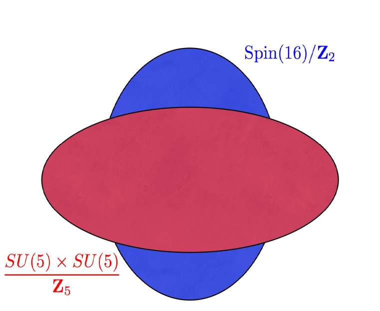
Figure 1: The $\mbox{Spin}(16)/{\bf Z}_{2}$ and $(SU(5)\times SU(5))/{\bf Z}_{5}$ subgroups of $E_{8}$.

For simplicity, we shall work on an elliptically-fibered $K3$ surface, and we shall build a stable $SU(5)$ bundle using Friedman-Morgan-Witten [32] technology. A rank 5 bundle with $c_{1}=0$, $c_{2}=12$ has a spectral cover in the lienar system $|5\sigma+12f|$ ($\sigma$ the class of the base, $f$ the class of the fiber in the elliptically-fibered surface), describing a curve of genus $g=5c_{2}-5^{2}+1=36$, together with a line bundle of degree $-(5+g-1)=-40$. The result is a (72-parameter) family of stable $SU(5)$ bundles with $c_{2}=12$ on $K3$, whose holonomy generically fills out all of $SU(5)$. If we put two together, and project to the ${\bf Z}_{5}$ quotient, the result is an $(SU(5)\times SU(5))/{\bf Z}_{5}$ bundle with connection that satisfies both anomaly cancellation and Donaldson-Uhlenbeck-Yau.

Moreover, this example is not unique – this describes a 144-dimensional family of examples. The lesson here is that such examples are not exotic special cases, but rather are very common, even generic.

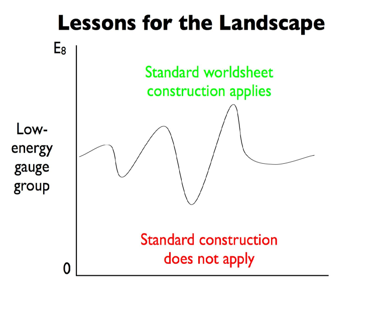
Figure 2: Low-energy gauge groups that can be described by the standard heterotic worldsheet construction.

Now that we have set up a problem, we shall see that in fact there is no swampland, by describing alternative worldsheet constructions that can describe more general $E_{8}$ bundles with connection. It should be emphasized, however, that even though these more general $E_{8}$ gauge fields can be described by some conformal field theory, there is a danger here for anyone doing statistics on standard worldsheet constructions – they do not capture all string vacua, only a misleading subset, as indicated schematically in figure 2.

We shall begin by describing more general ten-dimensional flat-space constructions. The basic idea is to replace Spin(16)/${\bf Z}_{2}$ with other subgroups of $E_{8}$, realized as orbifolds of abstract current algebras (since only $U(n)$ and Spin$(n)$ have level 1 free field representations).

To be specific, we shall describe $(SU(5)\times SU(5))/{\bf Z}_{5}$.

As a first check, let us consider the central charge. The central charge of a current algebra for an ADE group at level 1 is the same as the rank, so, the central charge of each $SU(5)$ is 4, hence the central charge of an $SU(5)\times SU(5)$ algebra at level 1 is 8, which will be unchanged by the ${\bf Z}_{5}$ orbifold. This is exactly right to match the central charge of $E_{8}$.

A more convincing test is to study the characters used to build a (hopefully modular-invariant) partition function. In the case of Spin(16)/${\bf Z}_{2}$, corresponding to the decomposition

$${\bf 248}\>=\>{\bf 120}\>+\>{\bf 128}$$

of the adjoint representation of $E_{8}$, there is a decomposition of characters

$$\chi_{E_{8}}({\bf 1},q)\>=\>\chi_{Spin(16)}({\bf 1},q)\>+\>\chi_{Spin(16)}({\bf 128},q)$$

which build the left-moving part of the heterotic partition function. (The adjoint representations are descendants of the identity operator in level 1 current algebras, and so are buried in the characters for ${\bf 1}$.)

In the case of $SU(5)^{2}/{\bf Z}_{5}$, from the decomposition

$${\bf 248}\>=\>({\bf 1},{\bf 24})\>+\>({\bf 24},{\bf 1})\>+\>({\bf 5},{\bf\overline{10}})\>+\>({\bf\overline{5}},{\bf 10})\>+\>({\bf 10},{\bf 5})\>+\>({\bf\overline{10}},{\bf\overline{5}})$$

of the adjoint representation of $E_{8}$, we get a prediction for the characters:

$$\chi_{E_{8}}({\bf 1},q)\>=\>\chi_{SU(5)}({\bf 1},q)^{2}\>+\>4\,\chi_{SU(5)}({\bf 5},q)\,\chi_{SU(5)}({\bf 10},q).$$

The $SU(5)$ characters can be shown to be

$$\chi_{SU(5)}({\bf 1},q) = \frac{1}{\eta(\tau)^{4}}\sum_{\vec{m}\in{\bf Z}^{4}}q^{\left(\sum m_{i}^{2}+(\sum m_{i})^{2}\right)/2}$$

$$\chi_{SU(5)}({\bf 5},q) = \frac{1}{\eta(\tau)^{4}}\sum_{\vec{m}\in{\bf Z}^{4},\sum m_{i}\equiv 1\>mod\>5}q^{\left(\sum m_{i}^{2}-\frac{1}{5}(\sum m_{i})^{2}\right)/2}$$

$$\chi_{SU(5)}({\bf 10},q) = \frac{1}{\eta(\tau)^{4}}\sum_{\vec{m}\in{\bf Z}^{4},\sum m_{i}\equiv 2\>mod\>5}q^{\left(\sum m_{i}^{2}-\frac{1}{5}(\sum m_{i})^{2}\right)/2}.$$

It can be shown [33, 34] that

$$\chi_{E_{8}}({\bf 1},q)\>=\>\chi_{SU(5)}({\bf 1},q)^{2}\>+\>4\,\chi_{SU(5)}({\bf 5},q)\,\chi_{SU(5)}({\bf 10},q),$$

which is exactly the desired character identity.

Let us go back and re-examine these statements more carefully. In the character decomposition for Spin(16)/${\bf Z}_{2}$, namely

$$\chi_{E_{8}}({\bf 1},q)\>=\>\chi_{Spin(16)}({\bf 1},q)\>+\>\chi_{Spin(16)}({\bf 128},q),$$

there is a ${\bf Z}_{2}$ orbifold implicit – the ${\bf 1}$ is from the untwisted sector, the ${\bf 128}$ from the twisted sector. Similarly, in the expression

$$\chi_{E_{8}}({\bf 1},q)\>=\>\chi_{SU(5)}({\bf 1},q)^{2}\>+\>4\,\chi_{SU(5)}({\bf 5},q)\,\chi_{SU(5)}({\bf 10},q),$$

there is a ${\bf Z}_{5}$ orbifold implicit – the ${\bf 1}$ is from the untwisted sector, the other four pieces are from four twisted sectors. This is exactly what we should find – the correct subgroup of $E_{8}$ is $SU(5)^{2}/{\bf Z}_{5}$, not $SU(5)^{2}$; there is a ${\bf Z}_{5}$ that should replace the left-moving ${\bf Z}_{2}$ GSO-analogue of the ordinary heterotic string construction.

It is straightforward to repeat this analysis for other subgroups of $E_{8}$. For example, let us next consider $SU(9)/{\bf Z}_{3}$. Again, the central charge of the current algebra at level 1 is 8, which matches that of the $E_{8}$ current algebra. From the decomposition of the $E_{8}$ conformal family

$$[{\bf 1}]\>=\>[{\bf 1}]\>+\>[{\bf 84}]\>+\>[{\bf\overline{84}}]$$

one predicts a character identity

$$\chi_{E_{8}}({\bf 1},q)\>=\>\chi_{SU(9)}({\bf 1},q)\>+\>2\,\chi_{SU(9)}({\bf 84},q)$$

and it can be shown that this is correct. Furthermore, note that in the expression above, there is a ${\bf Z}_{3}$ orbifold implicit, exactly as desired since the correct subgroup is $SU(9)/{\bf Z}_{3}$. So, we can also describe the $E_{8}$ degrees of freedom with $SU(9)/{\bf Z}_{3}$, with a ${\bf Z}_{3}$ orbifold replacing the left-moving ${\bf Z}_{2}$ GSO-analogue of the ordinary heterotic string construction.

For many other maximal-rank subgroups, there is an analogous story. For at least one non-maximal-rank, non-simply-laced subgroup, however, matters are more complicated. $E_{8}$ has a $G_{2}\times F_{4}$ subgroup, and one can check that the central charge of the $G_{2}\times F_{4}$ current algebra at level 1 is 8, exactly right to match that of $E_{8}$, and furthermore there is a character identity relating $\chi_{E_{8}}({\bf 1},q)$ to a sum over $G_{2}\times F_{4}$ characters, as needed. However, that character sum includes more terms that just characters of identity representations, terms which ordinarily would arise in twisted sectors of orbifolds, but there is no group-theoretic orbifold to perform: $G_{2}\times F_{4}$ has no finite center or indeed a finite normal subgroup that one could orbifold, and correspondingly the subgroup of $E_{8}$ is $G_{2}\times F_{4}$, not any quotient thereof. Therefore, although there exists formally a character decomposition, we do not understand how to realize it physically.

Next, in order to make this useful, we must describe how one fibers more general current algebras over spaces, in order to describe a compactified theory. To do this, we will outline fibered WZW models, first introduced by [35, 36, 37, 38, 39] under the name ‘lefton, righton Thirring models,” which we specialize to (0,2) theories.

Before describing fibered WZW models, let us first recall ordinary WZW models. An ordinary WZW model looks like a sigma model on the group manifold of a group $G$ together with $H$ flux:

$$S\>=\>-\frac{k}{2\pi}\int_{\Sigma}\mbox{Tr }\left[g^{-1}\partial gg^{-1}\overline{\partial}g\right]\>-\>\frac{ik}{2\pi}\int_{B}d^{3}y\epsilon^{ijk}\mbox{Tr }\left[g^{-1}\partial_{i}gg^{-1}\partial_{j}gg^{-1}\partial_{k}g\right].$$

The first term is the usual sigma model, the second or ‘Wess-Zumino’ term describes $H$ flux. This theory has a $G_{L}\times G_{R}$ symmetry, with currents

$$J(z)\>=\>g^{-1}\partial g,\>\>\>\overline{J}(\overline{z})\>=\>\overline{\partial}g\,g^{-1}$$

which (thanks to the Wess-Zumino term) obey

$$\overline{\partial}J(z)\>=\>\partial\overline{J}(\overline{z})\>=\>0.$$

These currents each realize a chiral $G$-Kac-Moody or current algebra at level $k$.

Next, let us describe how to fiber these WZW models. Let $P$ be a principal $G$ bundle over $X$, with connection $A$. Given an ordinary heterotic string worldsheet theory, the idea is that we shall replace the left-moving fermions $\lambda_{-}$ with a WZW model with left-multiplication gauged with the pullback of $A$. Schematically, the action has the form

$$\frac{1}{\alpha^{\prime}}\int_{\Sigma}\left(g_{i\overline{\jmath}}\partial_{\alpha}\phi^{i}\partial^{\alpha}\phi^{\overline{\jmath}}\>+\>\cdots\right)$$

$$\>\>-\>\frac{k}{4\pi}\int_{\Sigma}\mbox{Tr }\left(g^{-1}\partial gg^{-1}\overline{\partial}g\right)\>-\>\frac{ik}{12\pi}\int_{B}d^{3}y\epsilon^{ijk}\mbox{Tr }\left(g^{-1}\partial_{i}gg^{-1}\partial_{j}gg^{-1}\partial_{k}g\right)$$

$$\>\>-\>\frac{k}{2\pi}\mbox{Tr }\left((\partial\phi^{\mu})A_{\mu}\overline{\partial}gg^{-1}\>+\>\frac{1}{2}(\partial\phi^{\mu}\overline{\partial}\phi^{\nu})A_{\mu}A_{\nu}\right).$$

The first line describes a nonlinear sigma model on $X$; the second line describes a WZW model; the third line describes the operation of gauging left-multiplication. The third line will look very familiar to readers acquainted with gauged WZW models; the differences here are that we only gauge a chiral multiplication, and that the gauge field is the pullback of a gauge field on the target space, rather than a worldsheet gauge field.

Now, a WZW model action is invariant under gauging symmetric group multiplications, but not under the chiral group multiplications that we have here. Under

$$g \mapsto hg$$

$$A_{\mu} \mapsto hA_{\mu}h^{-1}\>+\>h\partial_{\mu}h^{-1}$$

the classical action is not invariant.

On the one hand, this lack of invariance is expected – this is the bosonization of the chiral anomaly. On the other hand, this lack of invariance creates a potential well-definedness issue in the fibered WZW construction.

The fix is a quantum correction which cancels the classical non-invariance. In particular, the classical action picks up a quantum correction across coordinate patches, due to the right-moving chiral fermion anomaly.

To make the action gauge-invariant, we proceed in the usual form, by assigning a transformation law to the $B$ field. To be able to do this globally implies that

$$k\,\mbox{ch}_{2}({\cal E})\>=\>\mbox{ch}_{2}(TX)$$

which is the analogue of the usual anomaly-cancellation condition for left-movers at level $k$. If this condition is obeyed, the action is well-defined globally.

Proceeding in the usual fashion for heterotic strings, the right-moving fermion kinetic terms on the worldsheet couple to $H$ flux:

$$\frac{i}{2}g_{\mu\nu}\psi_{+}^{\mu}D_{\overline{z}}\psi_{+}^{\nu}$$

where

$$D_{\overline{z}}\psi_{+}^{\mu}\>=\>\overline{\partial}\psi_{+}^{\mu}\>+\>\overline{\partial}\phi^{\mu}\left(\Gamma^{\nu}_{\>\>\sigma\mu}\>-\>H^{\nu}_{\>\>\sigma\mu}\right)\psi_{+}^{\sigma}.$$

To make the fermion kinetic terms gauge-invariant under the transformation of the $B$ field, we must redefine $H$ to be

$$H\>=\>dB\>+\>(\alpha^{\prime})\left(kCS(A)\>-\>CS(\omega)\right)$$

so that $H$ is a well-defined 3-form globally. This implies that

$$k\,\mbox{ch}_{2}({\cal E})\>=\>\mbox{ch}_{2}(TX)$$

which is, again, the anomaly cancellation condition.

Next, let us demand (0,2) supersymmetry. One discovers an old faux-supersymmetry-anomaly in subleading terms in $\alpha^{\prime}$ in the heterotic string, one originally discussed by [40, 41]. The supersymmetry transformations in the ordinary heterotic string worldsheet are:

$$\delta\lambda_{-}\>=\>-i\epsilon\psi_{+}^{\mu}A_{\mu}\lambda_{-}.$$

Note that this is the same as a chiral gauge transformation with parameter $-i\epsilon\psi_{+}^{\mu}A_{\mu}$. Because of the chiral anomaly in the ordinary heterotic worldsheet, this means there is a quantum contribution to the supersymmetry transformations at order $\alpha^{\prime}$. In our bosonized description, this quantum effect appears at leading order.

The one-fermi terms in the supersymmetry transformations of the various components of the action are as follows. The nonlinear sigma model on the base contributes

$$\frac{1}{\alpha^{\prime}}\int_{\Sigma}(i\alpha\psi^{\overline{\imath}})\overline{\partial}\phi^{\mu}\partial\phi^{\nu}\left(H\>-\>dB\right)_{\overline{\imath}\mu\nu}.$$

The WZW fibers contribute

$$-k\int_{\Sigma}(i\alpha\psi^{\overline{\imath}})\overline{\partial}\phi^{\mu}\partial\phi^{\nu}CS(A)_{\overline{\imath}\mu\nu}.$$

This is the bosonization of the faux-supersymmetry-anomaly discussed above. Finally, there is an additional quantum contribution, a faux-supersymmetry-anomaly arising from the right-moving fermions, which contributes

$$\int_{\Sigma}(i\alpha\psi^{\overline{\imath}})\overline{\partial}\phi^{\mu}\partial\phi^{\nu}CS(\omega)_{\overline{\imath}\mu\nu}.$$

In order for the one-fermi terms to cancel out, we see that

$$H\>=\>dB\>+\>\alpha^{\prime}\left(kCS(A)\>-\>CS(\omega)\right)$$

which is, again, the anomaly cancellation condition, the third time now that we have derived it. The three-fermi terms behave similarly.

Next, let us turn to the massless spectrum, or more properly the spectrum of chiral primaries. In an ordinary WZW model, the WZW primaries are associated to integrable representations of the group $G$. Here, for each integrable representation $R$ of the principal $G$ bundle $P$, we get an associated vector bundle ${\cal E}_{R}$. The chiral primaries are then easily checked to be given by $H^{*}(X,{\cal E}_{R})$ for each integrable representation $R$.

For an example, consider $G=SU(n)$ at level 1. Here, the integrable representations are the fundamental ${\bf n}$ and its exterior powers, hence the chiral primaries are counted by $H^{*}(X,\Lambda^{*}{\cal E})$, in agreement with old results [42].

These fibered WZW constructions realize the ‘new’ elliptic genera of Ando and Liu [43, 44]. Ordinary elliptic genera describe left-movers coupled to a level 1 current algebra; these elliptic genera, on the other hand, have left-moving level $k$ current algebras.

It would be very interesting if these elliptic genera could be applied to understand, for example, black hole entropy computations.

4 String compactifications on stacks

In this section we will review results in [45, 46, 47, 48, 49, 50], describing string compactifications on stacks and applications to gauged linear sigma models.

Stacks are a mild generalization of spaces, on which there exist functions, metrics, spinors, and all the other machinery one needs to make sense of strings.

One would like to understand string compactifications on stacks, not only to understand the most general possible string compactifications, but also because they often appear physically inside various constructions.

So, what is a stack? We can cover a stack with coordinate charts, just like a manifold. So, locally, a stack looks just like a space. Globally, on a manifold, across triple overlaps, the coordinate charts close to the identity. On a stack, across triple overlaps, the coordinate charts need only close up to an automorphism. In other words, locally a stack is just like a space – the difference is global.

How does one make sense of string compactifications on stacks concretely? Every smooth, Deligne-Mumford stack can be presented as a global quotient $[X/G]$ for $X$ a space and $G$ a group. To such a presentation, we associate a $G$-gauged sigma model on $X$.

Following that program, we quickly run into a potential problem. If to $[X/G]$ we associate a $G$-gauged sigma model, then

• $[{\bf C}^{2}/{\bf Z}_{2}]$ defines a two-dimensional conformal field theory,

• $[X/{\bf C}^{\times}]$ for $X=\left({\bf C}^{2}\times{\bf C}^{\times}\right)/{\bf Z}_{2}$ is an isomorphic stack, but $[X/{\bf C}^{\times}]$ defines a two-dimensional theory without conformal invariance.

Thus, there is a potential presentation-dependence problem: the same stack, presented in two different ways, is associated with distinct quantum field theories. Just like in the physical realization of derived categories, wehre an analogous problem arises, our proposal is that this presentation-dependence is fixed by renormalization-group flow. In other words, stacks classify endpoints of renormalization-group flow.

There are some potential problems with this program, reasons to believe that presentation-independence fails. One example involves deformation theory. The first check of a geometrical interpretation of any physical structure is to compare physical deformations to mathematical deformations, and in all previously-known cases, they match. For stacks, on the other hand, there is a mismatch: deformations of physical theories do not match mathematical deformations of stacks. Another example of a potential problem with the program outlined above involves cluster decomposition, or rather lack thereof, in the theories one associates to special kinds of stacks known as gerbes.

These potential problems can be fixed [45, 46, 47, 48, 49]. The results include: mirror symmetry for stacks, new Landau-Ginzburg models, physical calculations of quantum cohomology for stacks, and an understanding of noneffective quotients in physics.

For example, let us consider quantum cohomology. As outlined earlier, the quantum cohomology ring of ${\bf C}{\bf P}^{N}$ is ${\bf C}[x]/(x^{N+1}-q)$, a deformation of the classical cohomology ring ${\bf C}[x]/(x^{N+1})$. The quantum cohomology ring of a ${\bf Z}_{k}$ gerbe over ${\bf C}{\bf P}^{N}$ with characteristic class $-n\mbox{ mod }k$ is

$${\bf C}[x,y]/\left(y^{k}-q_{2},x^{N+1}-y^{n}q_{1}\right).$$

In particular, even though the gerbe is not a space, one can still make sense of notions familiar from ordinary spaces.

For another example, the Toda dual of ${\bf C}{\bf P}^{N}$ is described by the holomorphic function

$$W\>=\>\exp(-Y_{1})\>+\cdots\>+\>\exp(-Y_{N})\>+\>\exp(Y_{1}\>+\>\cdots\>+Y_{N}).$$

The analogous duals to ${\bf Z}_{k}$ gerbes over ${\bf C}{\bf P}^{N}$ are described by

$$W\>=\>\exp(-Y_{1})\>+\cdots\>+\>\exp(-Y_{N})\>+\>\Upsilon^{n}\exp(Y_{1}\>+\>\cdots\>+Y_{N})$$

where $\Upsilon$ is a character-valued field [45, 46, 47].

More generally, there exists a notion of toric stacks [51] which allows us to realize sigma models on many stacks in terms of simple two-dimensional gauge theories. Standard mirror constructions now produce discrete-valued fields [45, 46, 47], a new effect, which ties into the stacky fan description of [51].

We now believe that for banded, abelian $G$-gerbes on spaces $X$, (2,2) supersymmetric strings cannot distinguish between

• the gerbe itself,

• disjoint union of copies of $X$ (one for each character of $G$), with flat $B$ fields, determined by the image of the map

  $$H^{2}(X,G)\>\stackrel{{\scriptstyle G\rightarrow U(1)}}{{\longrightarrow}}\>H^{2}(X,U(1)).$$

In other words, these are described by the same conformal field theory. This fact comes up in mirror constructions, and the meaning of discrete-valued fields, and has impliciations for quantum cohomology computations [48].

This result can also be applied to understand gauged linear sigma models. For example, let us consider the GLSM for the complete intersection ${\bf P}^{7}[2,2,2,2]$. At the Landau-Ginzburg point, onehas a superpotential of the form

$$\sum_{a}p_{a}G_{a}(\phi)\>=\>\sum_{ij}\phi_{i}A^{ij}(p)\phi_{j}$$

where the $G_{a}$ are quadric polynomials, and the $A^{ij}(p)$ is an $8\times 8$ matrix with entries linear in the $p$’s, and the $\phi_{i}$ are the homogeneous coordinates on ${\bf P}^{7}$. In particular, this superpotential describes mass terms for the $\phi_{i}$, away from the locus $\{\det A=0\}$, leaving just the $p$ fields. Since the $p$ fields have charge $-2$, this describes a ${\bf Z}_{2}$ gerbe, which physics sees as a double cover. Altogether, the Landau-Ginzburg point describes a branched double cover of ${\bf P}^{3}$. This is a non-birational twisted derived equivalence, and a physical realization of Kuznetsov’s homological projective duality [50].

Although (2,2) models on gerbes decompose into a disjoint union, (0,2) models do not in general. Heterotic strings on gerbes with twisted bundles do not factorize into a disjoint union of target spaces. The prototype for such bundles is the “${\cal O}(1/k)$” line bundle over the ${\bf Z}_{k}$ gerbe ${\bf P}^{N}_{[k,k,\cdots,k]}$ on ${\bf P}^{N}$, defined by a Fermi superfield of (minimal) charge 1. More generally, heterotic strings on gerbes give an understanding of some of the two-dimensional (0,4) theories appearing in the geometric Langlands program. Implicit here is a lesson for the landscape program: many more string vacua may exist than previously enumerated.

5 Conclusions

In this talk we have outlined three recent developments pertinent to heterotic strings. First, we discussed recent progress in understanding nonperturbative corrections in heterotic strings. Second, we discussed a potential heterotic swampland – the inability of ordinary heterotic worldsheet constructions to describe most $E_{8}$ bundles with connection – and its resolution via the construction of new heterotic worldsheet CFT’s. Finally, we outlined string compactifications on stacks. These compactifications give new insight into many gauged linear sigma models, ranging from exotic-seeming GLSM’s with nonminimal charges, to seemingly ordinary GLSM’s which have novel geometries appearing at various limits of their Kähler moduli spaces, physically realizing Kuznetsov’s homological projective duality and Kontsevich’s noncommutative spaces. Heterotic string compactifications on special stacks known as gerbes appear to provide a new class of string compactifications.

References

- [1] M. Becker, L-S. Tseng, S-T. Yau, “Heterotic Kähler/non-Kähler transitions,” arXiv: 0706.4290.
- [2] K. Becker, M. Becker, J-X. Fu, L-S. Tseng, S-T. Yau, “Anomaly cancellation and smooth non-Kähler solutions in heterotic string theory,” Nucl. Phys. B751 (2006) 108-128, hep-th/0604137.
- [3] K. Becker, L-S. Tseng, “Heterotic flux compactifications and their moduli,” Nucl. Phys. B741 (2006) 162-179, hep-th/0509131.
- [4] K. Becker, M. Becker, K. Dasgupta, R. Tatar, “Geometric transitions, non-Kähler geometries and string vacua,” Int. J. Mod. Phys. A20 (2005) 3442-3448, hep-th/0411039.
- [5] A. Adams, M. Ernebjerg, J. Lapan, “Linear models for flux vacua,” hep-th/0611084.
- [6] A. Adams, “Conformal field theory and the Reid conjecture,” hep-th/0703048.
- [7] V. Braun, Y-H. He, B. Ovrut, T. Pantev, “The exact MSSM spectrum from string theory,” JHEP 0605 (2006) 043, hep-th/0512177.
- [8] V. Bouchard, M. Cvetic, R. Donagi, “Tri-linear couplings in a heterotic minimal supersymmetric standard model,” Nucl. Phys. B745 (2006) 62-83, hep-th/0602096.
- [9] S. Katz, E. Sharpe, “Notes on certain (0,2) correlation functions,” Comm. Math. Phys. 262 (2006) 611-644, hep-th/0406226.
- [10] E. Sharpe, “Notes on certain other (0,2) correlation functions,” hep-th/0605005.
- [11] E. Sharpe, “Notes on correlation functions in (0,2) theories,” hep-th/0502064.
- [12] A. Adams, J. Distler, M. Ernebjerg, “Topological heterotic rings,” hep-th/0506263.
- [13] J. Guffin, S. Katz, “Deformed quantum cohomology and (0,2) mirror symmetry,” arXiv: 0710.2354.
- [14] I. Melnikov, S. Sethi, “Half-twisted (0,2) Landau-Ginzburg models,” arXiv: 0712.1058.
- [15] J. McOrist, I. Melnikov, “Half-twisted correlators from the Coulomb branch,” arXiv: 0712.3272.
- [16] J. Guffin, E. Sharpe, “A-twisted Landau-Ginzburg models,” arXiv: 0801.3836.
- [17] J. Guffin, E. Sharpe, “A-twisted heterotic Landau-Ginzburg models,” arXiv: 0801.3955.
- [18] E. Silverstein and E. Witten, “Criteria for conformal invariance of models,” Nucl. Phys. B444 (1995) 161-190, hep-th/9503212.
- [19] P. Berglund, P. Candelas, X. de la Ossa, E. Derrick, J. Distler, and T. Hubsch, “On the instanton contributions to the masses and couplings of singlets,” Nucl. Phys. B454 (1995) 127-163, hep-th/9505164.
- [20] C. Beasley and E. Witten, “Residues and worldsheet instantons,” JHEP 0310 (2003) 065, hep-th/0304115.
- [21] R. Blumenhagen, R. Schimmrigk, A. Wisskirchen, “(0,2) mirror symmetry,” Nucl. Phys. B486 (1997) 598-628, hep-th/9609167.
- [22] R. Blumenhagen, S. Sethi, “On orbifolds of (0,2) models,” Nucl. Phys. B491 (1997) 263-278, hep-th/9611172.
- [23] R. Blumenhagen, “Target space duality for (0,2) compactifications,” Nucl. Phys. B513 (1998) 573-590, hep-th/9707198.
- [24] R. Blumenhagen, “(0,2) target space duality, CICY’s, and reflexive sheaves,” Nucl. Phys. B514 (1998) 688-704, hep-th/9710021.
- [25] A. Adams. A. Basu, and S. Sethi, “ duality,” hep-th/0309226.
- [26] M. Atiyah, “Complex analytic connections in fibre bundles,” Trans. Amer. Math. Soc. 85 (1957) 181-207.
- [27] D. Morrison and R. Plesser, “Summing the instantons: quantum cohomology and mirror symmetry in toric varieties,” Nucl. Phys. B440 (1995) 279-354, hep-th/9412236.
- [28] F. Cachazo, M. Douglas, N. Seiberg, E. Witten, “Chiral rings and anomalies in supersymmetric gauge theory,” JHEP 0212 (2002) 071, hep-th/0211170.
- [29] J. Distler, E. Sharpe, “Heterotic compactifications with principal bundles for general groups and general levels,” hep-th/0701244.
- [30] T. Banks, talk given at “String vacuum workshop” at Max-Planck Institute, Munich, November 2004, and elsewhere.
- [31] C. Vafa, “The string landscape and the swampland,” hep-th/0509212.
- [32] R. Friedman, J. Morgan, and E. Witten, “Vector bundles and F theory,” Comm. Math. Phys. 187 (1997) 679-743, hep-th/9701162.
- [33] E. Scheidegger, private communication.
- [34] V. Kac, M. N. Sanielevici, “Decompositions of representations of exceptional affine algebras with respect to conformal subalgebras,” Phys. Rev. D37 (1988) 2231-2237.
- [35] S. J. Gates, Jr., W. Siegel, “Leftons, rightons, nonlinear sigma models, and superstrings,” Phys. Lett. B206 (1988) 631-638.
- [36] D. Depireux, S. J. Gates, Jr., Q-H. Park, “Lefton-righton formulation of massless Thirring models,” Phys. Lett. B224 (1989) 364-372.
- [37] S. Bellucci, D. Depireux, S. J. Gates, Jr., “(1,0) Thirring models and the coupling of spin-zero fields to the heterotic string,” Phys. Lett. B232 (1989) 67-74.
- [38] S. J. Gates, Jr., S. Ketov, S. Kuzenko, O. Soloviev, “Lagrangian chiral coset constructions of heterotic string theories in (1,0) superspace,” Nucl. Phys. B362 (1991) 199-231.
- [39] S. J. Gates, Jr., “Strings, superstrings, and two-dimensional lagrangian field theory,” pp. 140-184 in Functional integration, geometry, and strings, proceedings of the XXV Winter School of Theoretical Physics, Karpacz, Poland (Feb. 1989), ed. Z. Haba, J. Sobczyk, Birkhauser, 1989.
- [40] A. Sen, “Local gauge and Lorentz invariance of the heterotic string theory,” Phys. Lett. B166 (1986) 300-304.
- [41] A. Sen, “Superspace analysis of local Lorentz and gauge anomalies in the heterotic string theory,” Phys. Lett. B174 (1986) 277-279.
- [42] J. Distler, B. Greene, “Aspects of (2,0) string compactifications,” Nucl. Phys. B304 (1988) 1-62.
- [43] K. Liu, “On modular invariance and rigidity theorems,” J. Diff. Geom. 41 (1995) 343-396.
- [44] M. Ando, “The sigma orientation for analytic circle-equivariant elliptic cohomology,” math.AT/0201092.
- [45] T. Pantev, E. Sharpe, “Notes on gauging noneffective group actions,” hep-th/0502027.
- [46] T. Pantev, E. Sharpe, “String compactifications on Calabi-Yau stacks,” Nucl. Phys. B733 (2006) 233-296, hep-th/0502044.
- [47] T. Pantev, E. Sharpe, “GLSM’s for gerbes (and other toric stacks),” Adv. Theor. Math. Phys. 10 (2006) 77-121, hep-th/0502053.
- [48] S. Hellerman, A. Henriques, T. Pantev, E. Sharpe, M. Ando, “Cluster decomposition, T-duality, and gerby CFT’s,” hep-th/0606034.
- [49] E. Sharpe, “Derived categories and stacks in physics,” contribution to proceedings of Vienna homological mirror symmetry conference, June 2006, hep-th/0608056.
- [50] A. Caldararu, J. Distler, S. Hellerman, T. Pantev, E. Sharpe, “Non-birational twisted derived equivalences in abelian GLSM’s,” arXiv: 0709.3855.
- [51] L. Borisov, L. Chen, and G. Smith, “The orbifold Chow ring of toric Deligne-Mumford stacks,” math.AG/0309229.