What Is There Between Any Two Nodes in a Complex Network?

Abstract

This article focuses on the identification of the number of paths with different lengths between pairs of nodes in complex networks and how, by providing comprehensive information about the network topology, such an information can be effectively used for characterization of theoretical and real-world complex networks, as well as for identification of communities.

I Introduction

A large number of natural and artificial complex systems can be represented and modeled in terms of networks involving interacting components. Such interactions can range from signalling between cells to social contacts (e.g.  Amaral04:EPJB ). Indeed, complex networks theory has been considered in a wide range of applications including neuronal connections, protein-protein interactions, economy, Internet communication and social ties costa2007aam , to cite just a few possibilities. It was thanks to their flexibility and potential for multidisciplinary applications that complex networks became so popular and important.

Much of the efforts by networks researchers have been concentrated in developing tools for characterization, classification, modeling and simulation. The characterization of network structure is one of the fundamental steps of complex networks research, because the modeling, simulation and classification of networks all depend strongly on accurate descriptions of the respective topology description  Costa_surv:2007 ; Boccaletti06 . In order to quantify different topological properties, a large set of network measurements has been developed Costa_surv:2007 . Many of these features are related to the concept of connectivity between nodes, taking into account the immediate links between each pair of nodes. Several of the measurements currently employed in order to characterize network structure – such as degree, clustering coefficient and shortest path length — are ultimately related to pairwise interconnectivity Costa_surv:2007 . It is therefore important to resort to longer range interaction between nodes in order to achieve more comprehensive description, characterization and modeling of complex structures. The average shortest path length (or geodesic distance) between a pair of nodes corresponds to one of such measurements Watts98:Nature . Usually, its average value is obtained considering the shortest distance between every pair of nodes. Some works have also considered distance matrices, containing minimum shortest path lengths, in order to enhance the characterization nicolelis1990scn ; Andrade2008ccn ; Bagrow2008pcn ; shavitt2007bcc and identification of isomorphisms Andrade2008ccn ; Bagrow2008pcn . Nevertheless, the isolated consideration of these measurement results in incomplete network characterization, since important information about network structure is not taken into account. For instance, the alternative paths between pair of nodes whose lengths are larger than the shortest path are completely overlooked by more traditional network analysis. Thus, two networks presenting the same degree and shortest path distributions, but different alternative paths organization, can be characterized as being identical, which is clearly inappropriate. Also, alternative paths can provide additional information about network resilience, once they generally reinforce connections, providing alternative routes and maximizing the flow. More traditional robustness analysis taking into account just the local connectivity and measurements related to the shortest paths, such as betweenness centrality Motter02:PRE and efficiency Latora01:PRL , also do not take into account the richer interconnectivity structure provided by longer alternative paths.

The comprehensive characterization of pairwise connectivity clearly requires more general approaches considering multi-scale interactions extending from the immediate link to long-range connectivity. The term multi-scale refers to the varying topological scales which are progressively taken into account around the nodes. The traditional approach considers just the first scale ($h=1$), i.e. immediate neighbor connectivity. In other words, in addition to immediate-connection measurements and limited long range information such as the shortest paths, the identification of alternative paths of any length can enhance the network characterization, providing a more complete description of network topology. Measurements taking into account the successive shortest path lengths from a reference node (concentric neighborhoods) have been proposed in the literature in terms of hierarchical or concentric representations Costa:2004 ; Costa_NJP:2007 ; Costa_JSP:2006 ; Costa_EPJB:2005 ; Costa_surv:2007 .

The further generalizations of the concepts of connectivity and interaction necessarily in order to account for larger portions of the network, requires the identification of alternative paths between pairs of nodes, as illustrated in Figure 1. Let us suppose we are interested in the pairwise interconnection between London (UK) and Lyon (France), which is particularly important for those people who have to travel by express train between those two cities. If we consider the shortest path approach, just the path of length three between those two cities is taken into account, while the other seven alternative paths are completely overlooked. Nevertheless, such paths are still fundamental for network communication and resilience. For instance, if the connection London-Paris-Lyon is blocked in any part other than from London to Lille, the train or passengers can always take the alternative routes. The importance of the identification of alternative paths in networks has also been substantiated with respect to the cardiovascular system nicolelis1990scn .

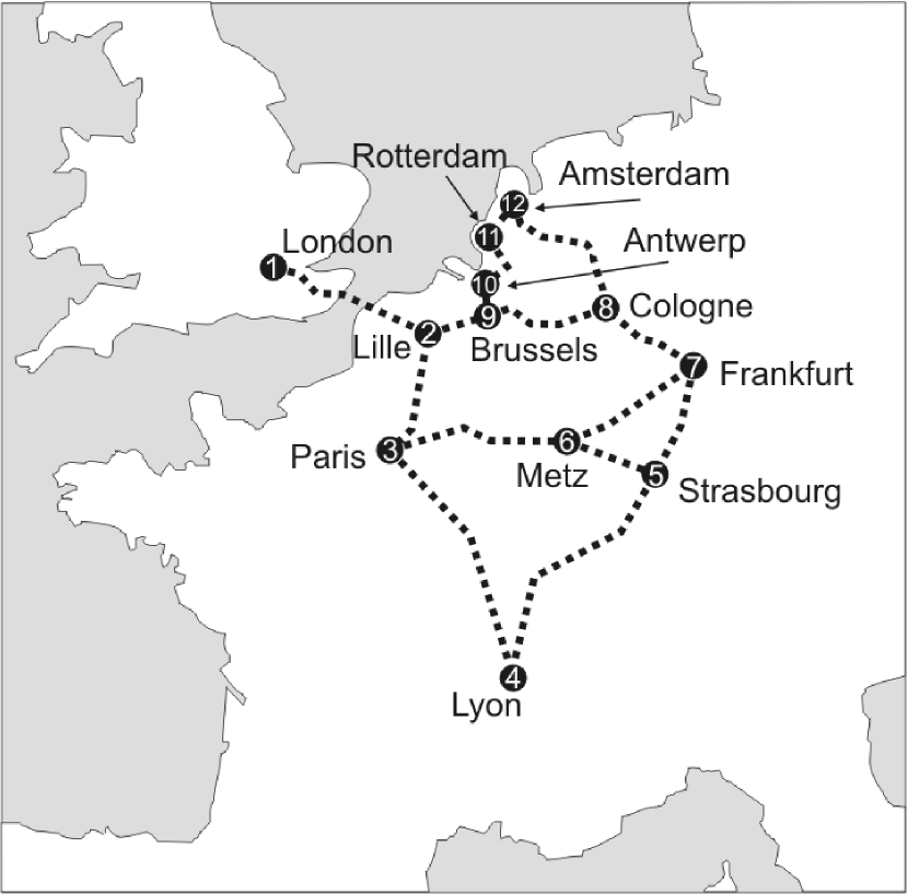
Figure 1: The European high-speed rail network connecting the main cities of central Europe. While the traditional network characterization in terms of the shortest distance takes into account just one path of length three between London and Lyon, the other seven alternative paths are overlooked. However, the alternative paths are fundamental for network topology and can be associated to important dynamics such as traffic jamming and resilience Boccaletti06 .

In the current article we report a comprehensive approach to generalize the concept of pairwise connectivity through the quantification of the distribution of paths of different lengths between pairs of nodes. The potential of such a framework is illustrated with respect to network characterization, with respect to both theoretical models and real-world networks, as well as community detection. Helped by optimal multivariate statistical methods, we characterize the relationships between the topologies of six distinct complex networks theoretical models and discuss the achieved discriminability. In order to illustrate the variation of the generalized connectivity in real-world networks, we report and discuss results corresponding to: (i) the US highway network, (ii) the neural C. elegans network Watts98:Nature , (iii) the cat cortical network sporns2004swc and (iv) a food web of a broadleaf forest in New Zealand Jaarsma1998cfw . In addition, we characterize the network modular structure (community) considering respective generalized connectivity matrices. The projection of the network vertices considering an optimal multivariate statistical method resulted in vertices belonging to the same communities being projected nearby, forming clusters of points.

In next sections, we provide the basic concepts related to network models, paths between nodes, principal component analysis (PCA) and network discriminability. An optimal algorithm to find the number of paths between pair of vertices is also provided. The illustration of the potential of the proposed methodology with respect to theoretical and real-world networks, as well as for community identification, are presented and discussed subsequently.

II Basic Concepts and methodology

An undirected network can be represented by its adjacency matrix $A$, whose elements $a_{ij}$ are equal to one whenever there is a connection between the vertices $i$ and $j$, or equal to zero otherwise. The number of connections of a given vertex $i$ is called its degree $k_{i}$, while the clustering coefficient $cc_{i}$, is defined as i.e. $cc_{i}=2n_{i}/(k_{i}-1)k_{i}$, where $n_{i}$ is the number of connections between the neighbors of $i$ Watts98:Nature . The number of paths with length $h=1,\ldots,H$ between each pair of nodes can be expressed in terms of the three-dimensional matrix $R=R(h,i,j)$ (see Figure 2), so that each matrix $R_{h}(i,j)=R(h,i,j)$ gives the total number of paths of length $h=1,2,\ldots,H$ extending from node $j$ to node $i$ (observe that $R_{1}=A$). These matrices will always be symmetric for undirected networks. The set of matrices $R_{h}$ therefore conveys comprehensive information about the generalized connectivity between any pair of nodes, therefore providing valuable additional information about the network structure. In addition, the shortest path distance matrix can be derived from such matrices by taking the minimum value along all matrices $R$ obtained for all possible $h$ (see Figure 2). Therefore, the matrices $A$ and $D$ are special cases of the set of matrices $R_{h}$. The matrix $T$, which is obtained by summing the elements along the set $R_{h}$, gives the number of paths of lengths $h=1,\ldots,H$ between every pair of vertices. As such, this matrix quantifies all alternative paths between pair of nodes and can be used, for instance, in analysis of network resilience.

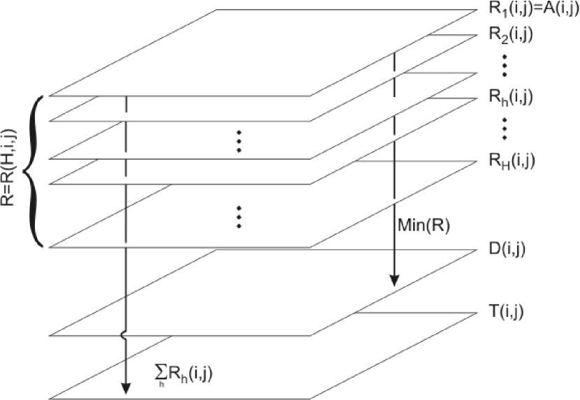
Figure 2: Networks can be characterized in terms of the three-dimensional matrix $R=R(H,i,j)$, which provides a more comprehensive description of the network structure than the traditional adjacency ($A(i,j)=R_{1}(i,j)$) and shortest paths length matrices ($D(i,j)=min(R(H,i,j))$). The matrix $T$, which provides the total number of paths between every pair of vertices $i$ and $j$, can be obtained by summing the elements of the matrices $R_{h}(i,j)$.

An illustration of the several connectivity approaches that can be applied in order to characterize the network in Figure 1 is provided in Figures 3 and 4. Figures 3 (a) and (b) show the traditionally adopted matrices of adjacency and the shortest path lengths distances, respectively. While the adjacency matrix $A$ indicates the immediate connectivity between pairs of nodes, the shortest path lengths matrix $D$ contains the number of edges along the shortest paths between each pair of nodes. On the other hand, the matrices in Figure 4 are rarely (if ever) considered in the literature and express other types of pairwise interactions between the nodes. In such a figure, the matrices $R_{2}$, $R_{3}$, $R_{4}$ and $R_{5}$ express the number of distinct paths of lengths $h=2$, $h=3$, $h=4$ and $h=5$ between each possible pair of nodes in the network in Figure 1, respectively. Observe that these matrices make explicit important information which cannot be easily inferred from any of the two previous matrices, $A$ and $D$. For instance, while matrix $D$ indicates that there is only one paths of length four between Strasbourg (France) and Antwerp (Belgium), the matrix $R_{5}$ indicates that there are four paths of length five and matrix $R_{4}$, a path of length four. Similarly, while the matrix $D$ indicates that there is a single shortest path of length two between Lyon (France) and Metz (France), the matrix $R_{2}$, shows two paths of length two, and the matrix $R_{3}$, one path of length three, all viable alternatives in the case of eventual disruption of the shortest path. The other matrices provide information about even longer alternative paths, of eventual interest for a tourist who wants to visit several nearby places. Therefore, the set of matrices $R$ can provide valuable additional information about the network structure, leading to more accurate network characterization and classification.

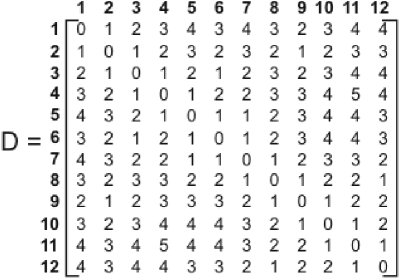
Figure 3: The adjacency (a) and distance (b) matrices, respective to the network in Figure 1.

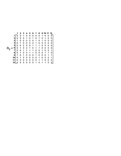
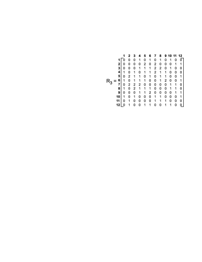
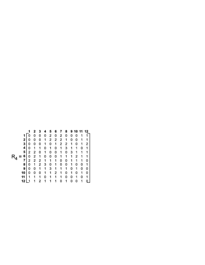
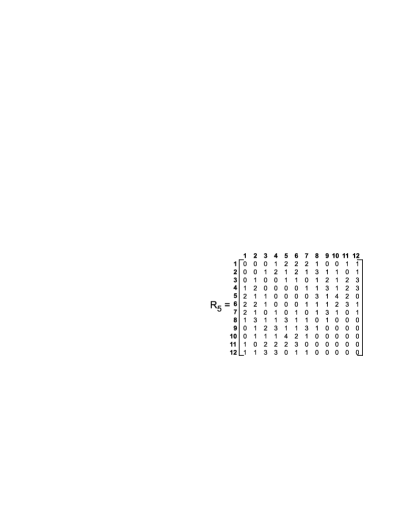
Figure 4: The matrices containing the number of paths of length $h=2$ (a), $h=3$ (b), $h=4$ (c) and $h=5$ (d) between each pair of nodes in the network in Figure 1.

II.1 Algorithm for identification of number of paths

The Algorithm 1 allows the identification of all paths between a reference vertex $i$ and all other nodes in a network. Such an optimal algorithm (each node is visited only once) can be applied to direct and undirected networks. The operations $push(a)$ and $pop(a)$ place and remove the data $a$ into a stack, respectively. Though this deterministic algorithm is optimal, it may require long periods of time depending on the type of network, its size, average degree, as well as the total number of steps $H$ required. Stochastic algorithms such as that described in Costa_comp:2007 ; Costa_longest:2007 can be considered for estimations in such cases. The execution of such an algorithm from all vertices on the network yields the set of matrices $R_{h}$.

Algorithm 1 The general algorithm to obtain the number of paths between each pair of vertices.

  for each vertex $i$ do

     $h=1$;

     $next$ = one of the non-visited immediate neighbors of $i$;

     $stack.push$(remainder of non-visited immediate neighbors of $i$, $h$);

     $path.push$($next$);

     $R(next,i,h)$ = 1;

     while stack not empty or size($path$) > 0  do

        $curr=next$;

        $ng$ = number of non-visited immediate neighbors of $curr$;

        if $ng$ > 0 then

           $next$ = one of the non-visited immediate neighbors of $curr$;

           $stack.push$(remainder of non-visited immediate neighbors of $curr$, $h$);

           $path.push$($next$);

        else

           $next,h$ = $stack.pop$(one node, $h$);

           $node=-1$;

           while $node\neq next$ do

              $node$ = $path.pop()$;

           end while

        end if

        $R(next,i,h)$ = $R(next,i,h)$ + 1;

     end while

  end for

II.2 Decorrelation of Measurements and Dimensionality Reduction

Because of the relatively high dimensionality of the path measurements, especially as a consequence of their parameterization with $h$, as well as the already observed correlations along $h$, it becomes important to consider means for obtaining effective projections of the measurements (dimensionality reduction) so as to visualize the network and vertex separations. This can be optimally performed through the method know as principal component analysis (PCA).

PCA can be defined as the orthogonal projection of the original data onto a lower dimensional linear space, called the principal subspace, such that the variance of the projected data is maximized along its first axes hotelling1933acs . Indeed, PCA can be understood as a rotation of the axes of the original variable coordinate system to new orthogonal axes in order to makes the new axes coincide with the directions of maximum variation of the original variables Costa:book . In practice, a PCA consists initially of finding the eigenvalues and eigenvectors of the sample covariance matrix bishop2006pra . So, let each of $Q$ observations (e.g. a node, a pair of nodes, or network), henceforth represented as $v=\{1,2,\ldots,Q\}$, be characterized in terms of $M$ respective features or measurements each, represented in terms of the feature vector $\vec{f_{v}}$ (each element $f_{v}(i)$, $i\in\{1,2,\ldots,M\}$, of this vector corresponds to one measurement of the observation $v$). For instance, we can consider the number of paths between each vertex $i$ and all other vertices in the network. In this case, each vertex presents a feature vector with $N$ elements. In cases where the number of features is large, it is possible to optimally reduce their dimensionality $M$ by removing the correlations between them. This important dimensional reduction transformation can be easily implemented by using the PCA methodology (e.g. Costa:book ; Costa_surv:2007 ).

Let the covariance between each pair of measurements $i$ and $j$ be given as

$$C(i,j)=\frac{1}{Q-1}\sum_{v=1}^{Q}(f_{v}(i)-\mu_{i})(f_{v}(j)-\mu_{j}),$$ (1)

where $\mu_{i}$ is the average of $f_{v}(i)$ over the $Q$ observations, i.e.

$$\mu_{i}=\frac{1}{Q}\sum_{v=1}^{Q}f_{v}(i).$$ (2)

The covariance matrix between these measurements is defined as $C=[C(i,j)]$, with dimension $M\times M$. Let the eigenvalues of $C$, sorted in decreasing order, be represented as $\lambda_{i}$, $i=1,2,\ldots,M$, with respective eigenvectors $\vec{v_{i}}$. By stacking such eigenvectors, it is possible to obtain the matrix

$$G=\left[\begin{array}[]{cccc}\uparrow&\uparrow&\ldots&\uparrow\\ \vec{v_{1}}&\vec{v_{2}}&\ldots&\vec{v_{m}}\\ \uparrow&\uparrow&\ldots&\uparrow\\ \end{array}\right],$$ (3)

which defines the stochastic linear transformation known as Karhunen-Loève transform Costa:book ; Costa_surv:2007 . Now, the new feature vectors can be obtained from the original measurement vectors $\vec{f}$ by making

$$\vec{g}=G\vec{f}.$$ (4)

The variances of the new measurements in $\vec{g}$ are provided by the respective eigenvalues. In case the measurements are correlated, most of their variances will be concentrated along the first elements of $\vec{g}$, which is guaranteed by the fact that the PCA completely decorrelates the original measurements. Indeed, the PCA is optimal with respect to concentrating the variation along the first axes. Therefore, it is possible to reduce the dimensionality of the features vectors by disregarding in the matrix in Equation 3 all eigenvectors associated to eigenvalues smaller than a given threshold, or by taking only the $R$ first eigenvectors. The resulting variables, which are fully uncorrelated linear combinations of the original measurements, concentrate the variance of the overall data and therefore represent a particularly meaningful characterization of the distribution of the original observations.

III Characterization of Theoretical Network Models

Six different types of theoretical network models are considered in this article. The Erdős-Rényi (ER) random graphs Erdos-Renyi59 are obtained by connecting $N$ initially isolated nodes with constant probability $p$. The traditional preferential attachment rule Barabasi1999 is used to obtain the scale-free Barabási-Albert (BA) networks. Such a model is a particular case of the Krapivsky et al. Krapivsky00 complex network model, which considers a non-linear preferential attachment rule to establish connections during network growth — the probability of connection is defined as $\mathcal{P}_{i\rightarrow j}=k_{j}^{\alpha}/\sum_{u}k_{u}^{\alpha}$, where $\alpha$ is the non-linear exponent. Observe that $\alpha=1$ yields the BA model. In order to obtain the Watts-Strogatz small-world model (WS), each connection in a linear lattice is rewired with probability $p$. Geographical networks (GN) are obtained by starting with $N$ nodes distributed uniformly along a three-dimensional space and connecting them according to distance, i.e. the probability to connect two vertices $i$ and $j$ is given by $P_{ij}=\lambda exp(-\lambda d_{ij})$, where $\lambda$ is a parameter to adjust the network degree and $d_{ij}$ is the Euclidean distance between $i$ and $j$. Such a model was introduced by Waxman to model the Internet topology waxman1988rmc . Knitted networks (KT) Costa_comp:2007 can be obtained by generating random sequences of nodes and connecting them sequentially (without repetition). The number of generated sequences depends on the network average connectivity. This network is particularly regular with respect to several of its topological and dynamical properties Costa_comp:2007 ; Costa_longest:2007 . In the current work, all these networks are grown with parameter sets so as to have the same number $N$ of nodes and approximately the same average degree.

In order to visualize the network distribution and separation (discriminability), the set of networks can be projected into a 3D space of decorrelated measurements. In the current work, we take into account as original measurements the averages and standard deviations of each matrix $R_{h}$. In this case, if we consider a maximum of $H$ distances, we have a set of $2H$ measurements, and each network is represented by a feature vector $\vec{v}=\{\mu_{1},\sigma_{1},\mu_{2},\sigma_{2},\ldots,\mu_{H},\sigma_{H}\}$, where $\mu_{h}$ and $\sigma_{h}$ are the average and standard deviation of the elements in the matrix $R_{h}$, respectively. The network projections obtained by the PCA reflect the network similarities in terms of their respective feature vectors. Indeed, models that are mapper nearby in the projected space tend to present similar topologies.

IV Community detection

Vertices belonging to the same community tend to present similar patterns of generalized connectivity, i.e. distributions of the number of paths of varying lengths. Since the generalized distance matrices provide comprehensive information about the distribution of paths between nodes, it can be considered for community detection. Thus, each vertex of a given network is represented by the feature vector $\vec{x_{i}}$ corresponding to the respective row (or column, as the distance matrices are symmetric) $i$ in the matrix $R_{h}$. Therefore, each element $j$ of such vector represents the number of paths of length $h$ between $i$ and $j$. The visualization of the vertex distribution can then be obtained by PCA projecting the feature vectors into the three-dimensional space. Thus, the vertices presenting similar set of attributes tend to be projected nearby, giving rise to clusters of points. Each of these clusters indicates a possible community in the original network.

V Results and Discussion

Our first experimental investigation concentrates in the characterization and discrimination between the topologies of six different complex networks theoretical models, namely: (i) the random graphs of Erdős and Rényi (ER), (ii) the small-world network model of Watts and Strogatz (WS), (iii) the geographical model of Waxman (GN), (iv) the scale-free model of Barabási and Albert (BA), (v) the non-preferential attachment model of Krapivsky et al. (NL) and (vi) the knitted network model of Costa (KT). We computed the averages and standard deviations of the matrices $R_{h}$ for $h=1,\ldots,6$, for each network model realization. In this way, each generated network is represented in terms of a vector with $12$ elements, i.e. the network $n$ is represented by the respective vector $\vec{v}_{n}=\{\mu_{1},\sigma_{1},\mu_{2},\sigma_{2},\ldots,\mu_{6},\sigma_{6}\}$, where $\mu_{h}$ and $\sigma_{h}$ stand for the average and standard deviation of the values in the matrix $R_{h}$. We generated 25 network realizations for each model and, after standardization, we projected those networks into the 3D space by applying the PCA methodology. As we can see in Figure 5, each of the respective types of networks generated by these models is represented by independent clusters of points (sharing similar topological properties), which indicates a clear separation between each network theoretical model. While the networks generated by preferential attachment rule (BA and NL, orange and cyan points) are organized at the right side of the projection, the most regular models (KT and ER, gray and blue points) are placed at the left side. Indeed, the scale-free networks tend to present greater variability of the number of paths than the more homogeneous models, once the presence of hubs tends to increase the number of paths between pairs of vertices and therefore generates a highly inhomogeneous path length distribution. In addition, the network models that generate networks with more regular structure tend to present the smallest cloud dispersions (KT and WS, gray and green points). In this way, by providing accurate discriminability between different models, the generalized connectivity approach presents good potential for enhancing network characterization and classification.

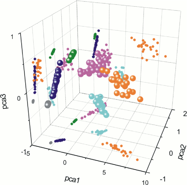
Figure 5: The projection of the networks generated by the ER (blue), WS (green), BA (orange), GN (magenta), KT (gray), and NL (cyan) network models in the 3-dimensional space.

In the case of the real-world networks, we applied our analysis to: (i) the US highway network, (ii) the neural C. elegans network Watts98:Nature , (iii) the cat cortical network sporns2004swc and (iv) a food web of a broadleaf forest in New Zealand Jaarsma1998cfw . Details about these networks are given in Table 1. Since these networks present different number of vertices and connections we cannot compare them directly – note that the number of paths for the cortical network is higher than for the other networks, which is a direct consequence of its higher average node degree. In this way, we considered the z-score in order to characterize the distribution of paths, which is calculated by Larsen1981ims

$$Z_{h}=\frac{\mu_{h}-\mu_{random}}{\sigma_{random}},$$ (5)

where $\mu_{h}$ is the average number of paths of length $h$ in the real network, and $\mu_{random}$ and $\sigma_{random}$ are the average and standard deviation of the number of paths in the respective randomized network ensemble, which were generated by the configuration model and present the same degree distribution as the respective real-world network Bender1978anl . The obtained results for the four network are presented in Table 1. It is interesting to note that just the neural network of the nematode C. elegans, which is the only case of a nervous system completely mapped at the level of neurons and chemical synapses Watts98:Nature , presents larger number of paths of lengths $h=2,3$ and $4$ than the randomized counterparts. For $h>4$, the randomized versions present higher number of paths. This suggests that connections of length $2,3,$ and $4$ could be more important for allowing proper dynamics in the C. elegans network. The highest difference for $h=3$ suggests that the evolution of the neuronal organization in this species tended to favor the alternative connections of length 3, while avoiding longer range connections. On the other hand, in case of the food web, the cortical network and the US highway, the z-scores tended to decrease with $h$, which indicates that such networks tend to present smaller number of paths of length $h>2$ than their randomized versions. Particularly, since food web tend to present a small number of trophic levels, there are no paths of length $h>4$, while the randomized version can display longer path sizes. Indeed, the small network diameter is a direct consequence of the energy transmission between trophic levels  power1990efr . In the case of the highway network, the fact that the randomized versions tended to present larger number of paths than the respective real-world version is a direct consequence of the fact that the connections in geographical highway network tend to be constrained by the adjacency between neighboring localities.

Table 1: The z-scores and the average number of paths obtained for the real-world networks.

Network	$N$	$\langle k\rangle$	$Z_{2}$	$\langle R_{2}\rangle$	$Z_{3}$	$\langle R_{3}\rangle$	$Z_{4}$	$\langle R_{4}\rangle$	$Z_{5}$	$\langle R_{5}\rangle$	$Z_{6}$	$\langle R_{6}\rangle$
Food web	78	3.1	0.002	0.05	-0.087	0.03	-0.12	0	-0.13	0	-0.11	0
Cortical net.	53	15.5	-0.027	5	-0.043	85	-0.06	1400	-0.08	21800	-0.11	331000
Neural net.	297	7.9	0.026	0.30	0.045	3	0.01	25	-0.05	210	-0.10	1750
US Highway	284	6.0	0	0.02	-0.048	2	-0.06	13	-0.06	100	-0.06	680

Our final analysis concentrated on the relationship between the modular network organization and the distribution of the number of alternative paths. Since vertices in the same community tend to present similar sets of more strongly connected nodes, the number of paths between the vertices in the same module tends to be large. We applied the proposed methodology described in Section IV to the Zachary karate club network and to an artificial modular network, which have been widely used as tests for community structure algorithms (e.g.Girvan2002css ). The karate club network was constructed with the data collected observing $34$ members of a karate club over a period of $2$ years and considering friendship between members Zachary1977ifm . On the other hand, the artificial network was generated as described in Girvan2002css , where a set of $N$ vertices is divided into $c$ communities. Then, each vertex is connected to $z_{in}$ vertices in the same community, and $z_{out}$ vertices in the other communities. The connections between communities are distributed uniformly. In the current work, we considered $N=128$, $c=4$, $z_{in}=10$ and $z_{out}=6$. From these networks, we calculated the respective $R_{h}$ matrices for $h=1,2$ and $3$. After standardization of the feature vectors, we applied the PCA and obtained the projections presented in Figure 6 and 7 for the karate and the artificial modular networks, respectively. In case of the Zachary karate club network, the best identification of the communities was obtained for $h=2$, where the classification of the vertices into the two clusters corresponds precisely to the actual division of the club members. The case $h=1$, which considers the traditional adjacency matrix, does not provide an accurate separation of the communities into different clusters. For $h\geq 3$, the separation is worse than for $h=2$ because the network presents a very small average shortest distance ($\ell=2.3$). Considering the shortest path matrix, the discriminability also resulted worse than that obtained for $R_{2}$. In the case of the artificial modular network, the best separation between the communities was also obtained for $h=2$, although for $h=3$ and $h=4$ the separation into four respective clusters is still clear. For the traditional matrices $A$ and $D$, two communities were all joined into the same cluster, therefore completely undermining the separation. It is interesting to note that most community finding algorithms cannot determine the communities perfectly for $z_{out}=6$ Boccaletti06 . Therefore, the consideration of the alternative paths can provide more information about the network structure and organization.

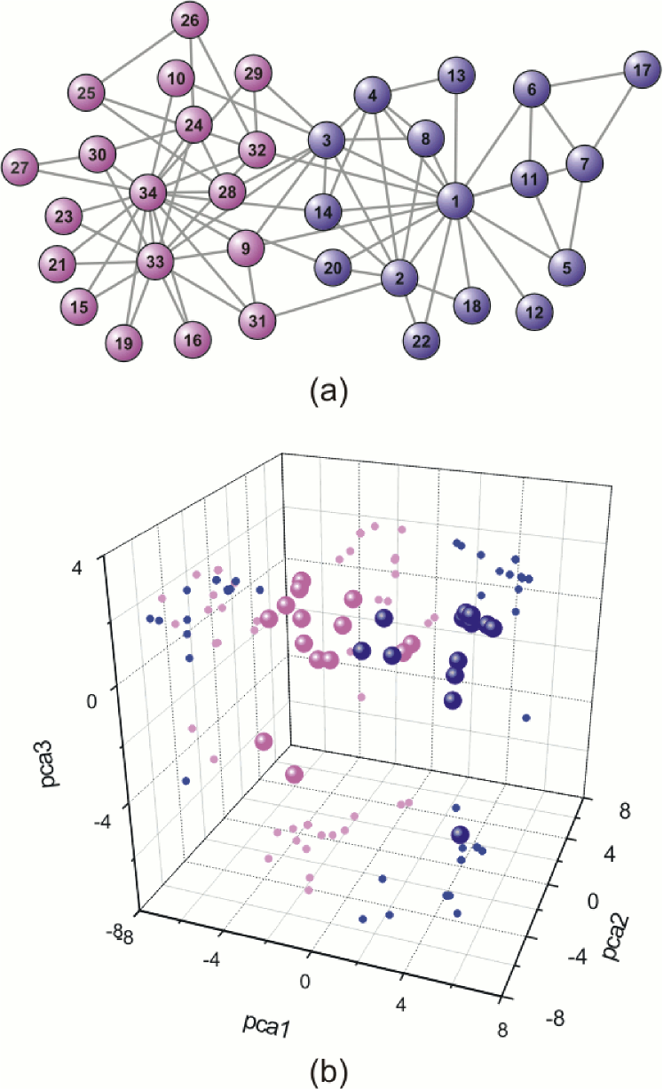
Figure 6: The original separation between the two classes of karate club member (a), and the projection into the three-dimensional space of the generalized matrix $R_{2}$.

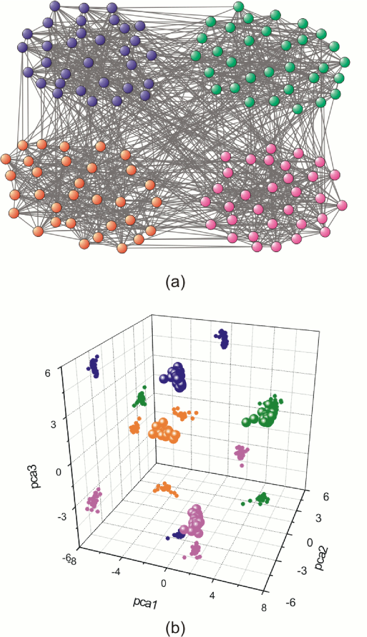
Figure 7: (a) The artificial network containing four communities and (b) the projection of the respective matrix $R_{2}$ into the three dimensional space considering the PCA methodology.

VI Concluding Remarks

The concept of connectivity underlies great part of the complex networks research. However, connectivity has typically been understood and quantified in terms either of strictly local measurements, such as the local degree, or by considering shortest path lengths. Though more global, the latter feature fails to take into account alternative pathways between pairs of nodes, which are extremely important in influencing the topological properties of the networks. For instance, the presence of more than one path between two nodes tends to increase the interaction between them and consequently raises their communication robustness under edge disruption.

In the current paper, we analyzed the generalized network connectivity with respect to the characterization of six network models and four real-world networks, as well as for community finding. We showed that the consideration of the alternative paths between vertices tends to provide an accurate network topology discriminability, as observed for the networks generated by the different models. The analysis of real-world networks suggests that the long range connectivity tend to be limited in those networks and may be strongly related to network evolution and organization. In addition, we studied how the distribution of the number of paths is related to network modular structure. The obtained results indicate that the proposed approach particularly promising for community identification. Indeed, a possibility for future work would be the improvement of the community analysis considering clustering methods to separate the cloud of points obtained in the projection, such as $k-$means or agglomerative hierarchical clustering Costa:book . In addition, pattern recognition approaches can be considered in order to quantify the separation between several types of networks models and therefore provide complex networks taxonomies. In this case, real-world networks can be associated to the most likely theoretical model, as described in Costa_surv:2007 . Studies relating the number of paths with network dynamics constitute another promising research possibility.

References

- [1] L. A. N. Amaral and J. M. Ottino. Complex networks. The European Physical Journal B, 38:147–162, 2004.
- [2] L. da F. Costa, O. N. Oliveira Jr, G. Travieso, F. A. Rodrigues, P. R. V. Boas, L. Antiqueira, M. P. Viana, and L. E. C. da Rocha. Analyzing and Modeling Real-World Phenomena with Complex Networks: A Survey of Applications. arXiv:0711.3199, 2008.
- [3] S. Boccaletti, V. Latora, Y. Moreno, M. Chavez, and D. U. Hwang. Complex networks: Structure and dynamics. Physics Reports, 424(4-5):175–308, 2006.
- [4] L. da F. Costa, F. A. Rodrigues, G. Travieso, and P. R. Villas Boas. Characterization of complex networks: A survey of measurements. Advances in Physics, 56(1):167 – 242, 2007.
- [5] D. J. Watts and S. H. Strogatz. Collective dynamics of small-world networks. Nature, 393(6684):440–442, 1998.
- [6] M. A. Nicolelis, C. H. Yu, and L. A. Baccala. Structural characterization of the neural circuit responsible for control of cardiovascular functions in higher vertebrates. Computers in Biology and Medicine, 20(6):379–400, 1990.
- [7] Y. Shavitt and Y. Singer. Beyond centrality classifying topological significance using backup efficiency and alternative paths. New Journal of Physics, 9:266, 2007.
- [8] R. F. S. Andrade, J. G. V. Miranda, S. T. R. Pinho, and T. P. Lobão. Characterization of complex networks by higher order neighborhood properties. The European Physical Journal B, 61(2):247–256, 2008.
- [9] J. P. Bagrow, E. M. Bollt, and J. D. Skufca. Portraits of complex networks. EPL (Europhysics Letters), 81:68004, 2008.
- [10] A. E. Motter and Y. C. Lai. Cascade-based attacks on complex networks. Physical Review E, 66(6):65102, 2002.
- [11] V. Latora and M. Marchiori. Efficient behavior of small-world networks. Physical Review Letters, 87(19):198701, 2001.
- [12] L. da F. Costa. The hierarchical backbone of complex networks. Physical Review Letters, 93:098702, 2004.
- [13] L. da F. Costa and R. F. S. Andrade. What are the best concentric descriptors for complex networks? New Journal of Physics, 9:311, 2007.
- [14] L. da F. Costa and F. N. Silva. Hierarchical characterization of complex networks. Journal of Statistical Physics, 125:845–876, 2006.
- [15] L. da F. Costa and L. E. C. da Rocha. A generalized approach to complex networks. The European Physical Journal B, 50:237–242, 2005.
- [16] O. Sporns and J. D. Zwi. The small world of the cerebral cortex. NeuroInformatics, 2(2):145–162, 2004.
- [17] N. G. Jaarsma, S. M. De Boer, C. R. Townsend, R. M. Thompson, and E. D. Edwards. Characterising food-webs in two New Zealand streams. New Zealand Journal of Marine and Freshwater Research, 32(2):271–286, 1998.
- [18] L. da F. Costa. Knitted complex networks. 2007. arXiv:0711.2736.
- [19] L. da F. Costa. Random and longest paths: Unnoticed motifs of complex networks. 2007. arXiv:0712.0415.
- [20] H. Hotelling. Analysis of a complex of statistical variables into principal components. Journal of Educational Psychology, 24(6):417–441, 1933.
- [21] L. da F. Costa and R. M. Cesar Jr. Shape Analysis and Classification: Theory and Practice. CRC Press, 2001.
- [22] C. M. Bishop. Pattern Recognition and Machine Learning. Springer-Verlag New York,USA, 2006.
- [23] P. Erdős and A. Rényi. On random graphs. Publicationes Mathematicae, 6:290–297, 1959.
- [24] A.-L. Barabási and R. Albert. Emergence of scaling in random networks. Science, 286:509, 1999.
- [25] P. L. Krapivsky, S. Redner, and F. Leyvraz. Connectivity of growing random netwoks. Physical Review Letters, 85(4629), 2000.
- [26] B. M. Waxman. Routing of multipoint connections. Selected Areas in Communications, IEEE Journal on, 6(9):1617–1622, 1988.
- [27] R. J. Larsen and M. L. Marx. An introduction to mathematical statistics and its applications. Prentice-Hall, 1981.
- [28] E. A. Bender and E. R. Canfield. The asymptotic number of labeled graphs with given degree sequences. Journal of Combinatorial Theory, Series A, 24(3):296–307, 1978.
- [29] M. E. Power. Effects of Fish in River Food Webs. Science, 250(4982):811, 1990.
- [30] M. Girvan and M. E. J. Newman. Community structure in social and biological networks. Proceedings of the National Academy of Sciences, 99(12):7821, 2002.
- [31] W. W. Zachary. An information flow model for conflict and fission in small groups. Journal of Anthropological Research, 33(4):452–473, 1977.