A semi-parametric technique for the quantitative analysis of Dynamic contrast-enhanced MR images based on Bayesian P-Splines

Abstract

Dynamic Contrast-enhanced Magnetic Resonance Imaging (DCE-MRI) is an important tool for detecting subtle kinetic changes in cancerous tissue. Quantitative analysis of DCE-MRI typically involves the convolution of an arterial input function (AIF) with a nonlinear pharmacokinetic model of the contrast agent concentration. Parameters of the kinetic model are biologically meaningful, but the optimization of the non-linear model has significant computational issues. In practice, convergence of the optimization algorithm is not guaranteed and the accuracy of the model fitting may be compromised. To overcome this problems, this paper proposes a semi-parametric penalized spline smoothing approach, with which the AIF is convolved with a set of B-splines to produce a design matrix using locally adaptive smoothing parameters based on Bayesian penalized spline models (P-Splines). It has been shown that kinetic parameter estimation can be obtained from the resulting deconvolved response function, which also includes the onset of contrast enhancement. Detailed validation of the method, both with simulated and in vivo data, is provided.

I Introduction

Evaluation of tissue kinetics in cancer with Dynamic Contrast-Enhanced Magnetic Resonance Imaging (DCE-MRI) has become an important tool for cancer diagnosis and quantification of the outcome of cancer therapies [2]. For DCE-MRI, after the administration of a contrast agent, such as Gadolinium diethylenetriaminepentaacetic acid (Gd-DTPA), a dynamic imaging series is acquired. Typically, $T_{1}$-weighted sequences are used to assess the reduction in $T_{1}$ relaxation time caused by the contrast agent. The contrast agent concentration time series can be estimated from the observed signal intensity using proton density weighted MRI after calibration or using multiple flip angle sequences [3, 4]. With Gd-DTPA, the agent does not enter into cells, so DCE-MRI depicts exchange between the vascular space and the extra-vascular extra-cellular space (EES).

Current approaches to quantitative analysis of DCE-MRI generally rely on non-linear pharmacokinetic models. These models are usually derived from the solution to a system of linear differential equations, which describe the blood flow in the tissue[5]. In practice, single-compartment models may not always be suitable, and thus more complex models have been suggested. They include the “extended” Tofts–Kermode model (see Eqn. 2) and the tissue homogeneity approach [6, 7]. However, non-linear regression models are difficult to optimize and the estimation of the parameters depends on the initial values of the algorithm [6].

Recently, model-free techniques have received extensive attention in quantitative imaging. Neural networks are used for tissue classification [8, 9] and semi-parametric methods in the kinetic modeling of dynamic PET imaging [10, 11]. For the quantification of first-pass myocardial perfusion, Jerosch-Herold et al. [12] proposed a model-free approach. The formulation of the response function based on a B-spline polynomial representation, however, is ill-conditioned and a first-order difference penalty spline (Tikhonov regularization) has been imposed.

As an alternative, Bayesian inference has also been investigated to replace traditional least-square fitting algorithms in MRI [13, 14]. Bayesian methods allow a more accurate description of the estimation uncertainty and can effectively reduce bias [15]. Furthermore, Bayesian hierarchical models can incorporate contextual information in order to reduce estimation errors [16]. A popular, general approach for semi-parametric modeling is based on Penalty splines, or P-splines [17, 18]. The function under consideration is approximated by a linear combination of a relatively large number of B-spline basis functions. A penalty based on $k$-th order differences of the parameter vector ensures smoothness of the function. For selecting the penalty weight (or smoothing parameter), the L-curve method [19] or cross validation can be used. In Bayesian frameworks, P-splines regression parameters can be estimated jointly with the penalty weight and hence allow for adaptive smoothing [20, 21].

In this paper, we propose a Bayesian P-spline model to fit the observed contrast agent concentration time curves. The model uses a locally adaptive smoothing approach as the observed time series signal varies rapidly in the first minute after injecting the contrast bolus. The proposed algorithm provides a semi-parametric deconvolution approach and results in a smooth response function, along with the corresponding estimates of uncertainty. Kinetic parameters are robustly derived by fitting a non-linear model to the estimated response function. In addition, the exact onset of the contrast uptake can be determined by using information derived from the Bayesian estimation process. Detailed validation of the method both with simulated and in vivo data of patients with breast tumors is provided.

II Theory and Methods

II-A Standard kinetic models for DCE-MRI

The standard parametric model for analyzing contrast agent concentration time curves (CTCs) in DCE-MRI is a single-compartmental model [22], where the solution can be expressed as a convolution of the arterial input function (AIF) with a single exponential function [23], i.e.,

$$C_{t}(t)=C_{p}(t)\otimes K^{\text{trans}}\exp(-k_{\text{ep}}t).$$ (1)

Here, $C_{t}(\cdot)$ denotes the concentration of the contrast agent, $C_{p}(\cdot)$ denotes the AIF, $K^{\text{trans}}$ represents the volume transfer constant between blood plasma and EES, and $k_{\text{ep}}$ represents the rate constant between EES and blood plasma. In this study, we use an extended version of the Tofts–Kermode model [6] as a reference parametric model given by

$$C_{t}(t)=v_{p}C_{p}(t)+C_{p}(t)\otimes K^{\text{trans}}\exp(-k_{\text{ep}}t),$$ (2)

where the additional parameter $v_{p}$ represents the fraction of contrast agent in the vascular compartment of the tissue.

The arterial input function $C_{p}$ describes the input of the contrast agent into the tissue. DCE-MRI studies typically use a standardized double exponential AIF given by [24]

$$C_{p}(t)=D\sum_{i=1}^{2}a_{i}\exp(-m_{i}t)$$ (3)

with values $a_{1}=24$ kg/l, $a_{2}=6.2$ kg/l, $m_{1}=3.00$ min^-1 and $m_{2}=0.016$ min^-1 [25]. In Eqn. 3, $D$ is the actual dosage of tracer in mmol/kg. With this explicit form of the AIF, the convolution in Eqn. 2 can be derived analytically, i.e.,

$$C_{t}(t)=v_{p}D\sum_{i=1}^{2}a_{i}\exp(-m_{i}t)+DK^{\text{trans}}\sum_{i=1}^{2}\frac{a_{i}\{\exp(-m_{i}t)-\exp[-k_{\text{ep}}t]\}}{k_{\text{ep}}-m_{i}}.$$ (4)

The kinetic parameters $K^{\text{trans}}$, $k_{\text{ep}}$ and $v_{p}$ are estimated by fitting Eqn. 4 to the observed data. Optimization is usually performed using the Levenberg–Marquardt algorithm [26].

II-B Bayesian P-Spline model for DCE-MRI

Parametric models, however, may not give an accurate fit of the observed data, as they are too simplistic and can overlook effects such as flow heterogeneity or the water exchange effect [27, 28]. More complex models have since been developed [7], but they are more difficult to optimize. It has been found that semi-parametric models can fit the data more accurately and in this study penalty splines (P-Splines) in a Bayesian hierarchical framework are used.

II-B1 Discrete Deconvolution

Mathematically, a more general expression of Eqn. 1 can be written as:

$$C_{t}(t)=C_{p}(t)\otimes f(t),$$ (5)

where $f(t)$ is the response function in the tissue. Assuming that $C_{p}(\cdot)$ and $f(\cdot)$ are constant over small intervals $\Delta t$, a discretized form of Eqn. 5 is given by

$$C_{t}(\tau_{i})=\sum_{j=1}^{T}C_{p}(\tau_{i}-t_{j})\,f(t_{j})\Delta\,t=\sum_{j=1}^{T}A_{ij}f(t_{j}),$$ (6)

where $C_{t}$ is measured on discrete time points $\tau_{1}\,\ldots,\tau_{n}$. The $n{\times}T$ matrix $\boldsymbol{A}$ may be interpreted as a convolution operator and is defined by

$$A_{ij}=\left\{\begin{array}[]{ll}C_{p}(t_{n_{i}-j+1})\Delta~{}t&\text{if $\tau_{i}\leq t_{j}$};\\ 0&\text{otherwise},\end{array}\right.$$ (7)

where $n_{i}$ is the maximum index $j$ for which $\tau_{i}\leq t_{j}$ holds. It is worth noting that the input function $C_{p}(t)$ is measured – or evaluated from Eqn. 3 – at time points $t_{1},\ldots,t_{T}$, which can be different from $\tau_{1},\ldots,\tau_{n}$.

II-B2 Penalty Splines

By solving Eqn. 6, the response function $f(t)$ can be deconvolved from $C_{p}(t)$. However, this system may be numerically unstable, i.e., the deconvolved response function is susceptible to noise. To overcome this problem, we assume that $f(t)$ is a smooth, $k$-times differentiable function. To this end, a B-spline representation of the response function is used in this study, i.e.,

$$f(t)=\sum_{j=1}^{p}\beta_{j}B_{tj},$$ (8)

where $\boldsymbol{B}$ is the $n{\times}p$ design matrix of $k$th order B-splines with knots $s_{1},\ldots,s_{p+k}$. In vector notation $\boldsymbol{f}=(f(t_{1}),\ldots,f(t_{T}))^{\prime}$ and Eqn. 8 may be expressed as

$$\boldsymbol{f}=\boldsymbol{B}\boldsymbol{\beta}.$$ (9)

Accordingly, Eqn. 6 can be written as

$$\boldsymbol{C_{t}}=\boldsymbol{A}\boldsymbol{f}=\boldsymbol{A}\boldsymbol{B}\boldsymbol{\beta}=\boldsymbol{D}\boldsymbol{\beta},$$ (10)

where $\boldsymbol{D}=\boldsymbol{A}\boldsymbol{B}$ is a $n{\times}p$ design matrix, representing the (discrete) convolution of the AIF with the B-spline polynomials.

To enhance the numerical stability, a penalty on the B-spline regression parameters is introduced, such that

$$\beta_{t}=2\beta_{t-1}-\beta_{t-2}+e_{t}\qquad\text{for $t=3,\ldots,p$}.$$ (11)

These models are known as penalty splines or P-Splines [17, 18] as they penalize the roughness of the function $f(t)$, and therefore act as a denoising method. As $\boldsymbol{C_{t}}$ exhibits a sharp initial increase followed by a sharp decrease at the beginning of the dynamic series, the penalty has to be locally adaptive. To this end, we use a Bayesian hierarchical framework for parameter inference.

II-B3 Bayesian hierarchical framework

In Bayesian inference, a priori information, i.e., information available before observation of measurement, has to be expressed in terms of probability distributions. Here, our prior knowledge is the assumption about the model. In this paper, we assume that the observed contrast agent concentration $\boldsymbol{C_{t}}$ is noisy realization of the true model (Eqn. 10), i.e.,

$$C_{t}(t)\sim\text{N}(\boldsymbol{D}_{t}\boldsymbol{\beta},\sigma^{2})\quad\text{for all $t$},$$ (12)

where $\boldsymbol{D}_{t}$ denotes the $t$th row of $\boldsymbol{D}$. That is, a priori the error is assumed to be Gaussian distributed with unknown variance $\sigma^{2}$. We use a relatively flat prior for the variance parameter, i.e.,

$$\sigma^{2}\sim\mbox{IG}(1,10^{-5}),$$ (13)

where IG denotes the Inverse Gamma distribution.

The penalty in Eqn. 11 can be expressed as a priori distribution on $\beta$ [21],

$$\beta_{t}\sim\text{N}(2\beta_{t-1}-\beta_{t-2},\delta_{t}^{2})\qquad\text{for $t=3,\ldots,p$},$$ (14)

where $\delta_{t}^{2}$ is the variance of $e_{t}$. For a locally adaptive estimation of $\delta_{t}^{2}$, the following prior model is used

$$\delta_{i}^{2}\sim\text{IG}(10^{-5},10^{-5})\qquad\text{ for $i=3,\ldots,p$},$$ (15)

which allows time varying smoothness penalties.

II-B4 Evaluation of the posterior distribution

Bayes’ theorem was used to calculate the posterior distribution of the parameter vector which is, up to a normalizing constant, given by

$$p(\boldsymbol{\beta},\boldsymbol{\delta^{2}},\boldsymbol{\sigma^{2}})\propto\ell(\boldsymbol{C_{t}}|\boldsymbol{\beta},\boldsymbol{\sigma^{2}})p(\boldsymbol{\sigma^{2}})p(\boldsymbol{\beta}|\boldsymbol{\delta^{2}})p(\boldsymbol{\delta^{2}}).$$ (16)

A closed-form solution of Eqn. 16 is not possible, and thus, Markov chain Monte Carlo (MCMC) techniques have been used to assess the posterior distribution [29]. The full conditional of $\boldsymbol{\beta}$, i.e., the joint distribution of $\boldsymbol{\beta}$ given all other parameters and the data, $\boldsymbol{C_{t}}$, is a $p$-dimensional multivariate normal distribution

$$\boldsymbol{\beta}|\boldsymbol{C_{t}},\boldsymbol{\delta^{2}},\boldsymbol{\sigma^{2}}\sim\mbox{\bf N}_{p}\left(\boldsymbol{C_{t}}^{\prime}\boldsymbol{D}(\boldsymbol{D}^{\prime}\boldsymbol{D}+\boldsymbol{R})^{-1},\sigma^{2}(\boldsymbol{D}^{\prime}\boldsymbol{D}+\boldsymbol{R})^{-1}\right),$$ (17)

where $\boldsymbol{R}$ is the inverse covariance matrix of the prior distribution of $\boldsymbol{\beta}$ [21]. The full conditionals of both variance parameters are independent Inverse Gamma distributions

$$\delta^{2}_{t}|\boldsymbol{\beta} \stackrel{{\scriptstyle iid}}{{\sim}} \mbox{IG}\left(10^{-5}+0.5,\,10^{-5}+0.5(\beta_{t}-2\beta_{t-1}+\beta_{t-2})\right)\text{ \quad for }t=3,\ldots,p,$$ (18)

$$\sigma^{2}|\boldsymbol{\beta},\boldsymbol{C_{t}} \sim \mbox{IG}\left(1+\frac{T}{2},\,10^{-5}+0.5(C_{t}-\boldsymbol{D_{t}}\boldsymbol{\beta})^{\prime}(C_{t}-\boldsymbol{D_{t}}\boldsymbol{\beta})\right).$$ (19)

To assess the posterior distribution, samples of the parameters $\boldsymbol{\beta},\sigma^{2}$ and $\boldsymbol{\delta}^{2}$ are drawn alternately from Eqn. 17, Eqn. 18 and Eqn. 19. After a sufficient burn-in period, the MCMC algorithm produces samples from the posterior distribution.

II-C Estimating kinetic parameters from the semi-parametric technique

The advantage of parametric models defined by Eqns. 1 and 2 is that they contain biologically meaningful and interpretable parameters. The semi-parametric technique only provides a fit to the CTC and a de-convolved and de-noised response function, but not kinetic parameters. In this section, we introduce methods for estimating kinetic parameters and the onset of the contrast uptake from the estimated response function. We make use of the fact that the Bayesian approach provides a rich source of information via the posterior distribution of the response function.

II-C1 Determining the onset of contrast uptake

In practice, the time delay between the injection of the contrast agent and the arrival of the tracer in the tissue of interest is unknown. However, it is important to correctly estimate the delay for a robust estimation of the kinetic parameters [30]. The Bayesian approach yields information on the uncertainty for each parameter in the model and for all transformations of the parameters such as the estimated contrast agent concentration $\boldsymbol{C_{t}}=\boldsymbol{D}\boldsymbol{\beta}$. This results in a point wise Credible Interval (CI) for the contrast agent concentration. From this, we can compute the minimal time $t^{*}$, where the 99% CI does not cover 0. That is, at time $t^{*}$ we are 99% confident that the contrast agent has already entered the tissue.

Assuming that the initial slope of the contrast agent concentration time curve is approximately linear, we can compute the onset time by drawing a line from $C_{t}(t^{*})$ to 0 with the gradient $dC_{t}(t^{*})/dt$. The first order derivative of $C_{t}(t^{*})$ can be computed by

$$\frac{d}{dt}C_{t}(t)=\frac{d}{dt}\left[C_{p}(t)\otimes f(t)\right]=C_{p}(t)\otimes\frac{d}{dt}f(t).$$

Since $f(t)$ is a spline, the derivative can be computed as [31]

$$f(t)=\sum_{j=1}^{n-k}\gamma_{j}B_{t(j+1)}^{(k-1)},$$

where $\boldsymbol{B^{(k-1)}}$ is the design matrix of $(k-1)$th order B-Splines and $\gamma_{j}$ is defined via

$$\gamma_{j}=\frac{k}{s_{j+k+1}-s_{j+1}}(\beta_{j+1}-\beta_{j})\text{ for }j=1,\ldots,J-1.$$

In this paper, we propose the following algorithm to estimate the onset of the contrast uptake:

1. Find the minimum time $t^{*}$, for which the contrast concentration significantly exceeds zero,

2. Compute the gradient of the estimated CTC at $t^{*}$,

3. Calculate the enhancement onset time as $t_{0}=t^{*}-\frac{C_{t}(t^{*})}{dC_{t}(t^{*})/dt}$.
   

DCE-MRI studies typically assume that the onset of the enhancement is the same over the whole region of interest (ROI). In this case, the median of the estimated $t_{0}$ for all voxels in the ROI may be used as an estimate of the global value. However, for larger ROIs, local estimates of the onset may be required, and can be computed from the proposed technique.

II-C2 Obtaining kinetic parameters

The semi-parametric technique provides a de-convolved and de-noised response function. In order to obtain kinetic parameters, we can fit a non-linear function to the estimated response. To this end, the following model has been used:

$$f(t)=F_{p}\cdot\left\{\begin{array}[]{ll}E\exp[-(t-t_{0}-T_{c})EF_{p}/v_{e}]&\text{for $t\geq(T_{c}+t_{0})$},\\ 1&\text{for $t_{0}\leq t<(T_{c}+t_{0})$},\\ 0&\text{for $t<t_{0}$},\\ \end{array}\right.$$ (20)

where $T_{c}=v_{p}/K^{\text{trans}}$ is the transit time through the capillary, $v_{e}=K^{\text{trans}}/k_{\text{ep}}$ is the volume fraction of EES, $E$ is the extraction fraction, and $F_{p}$ is the mean plasma flow. This model is similar to the adiabatic approximation of tissue homogeneity (AATH) [7]. In this model extraction fraction $E$ and mean plasma flow $F_{p}$ may be not identifiable, but the product $EF_{p}=K^{\text{trans}}$ is.

It should be noted that the Bayesian methodology provides not just one response function, but a (posterior) distribution of response functions. In order to obtain a distribution of the estimated parameters, the model in Eqn. 20 can be fitted to each response function in the sample using the Levenberg–Marquardt optimization algorithm. The median of the posterior distributions may be used to estimate the parameters. The estimation error can be computed using the standard errors across the samples and intervals can be constructed from quantiles of the posterior distributions.

II-D Data Collection

Simulated DCE-MRI data of CTCs with known kinetic parameters were previously published in [6]. We use the first series which was designed to be representative of data acquired from a breast tumor. Data was simulated using MMID4, part of a software made available by the National Simulation Resource, Dept. of Bioengineering, University of Washington (http://www.nsr.bioeng.washington.edu). Estimates from the literature were used as baseline values. For twelve further experiments, one of the kinetic parameters $F_{p}$, $v_{p}$ and $PS$ was changed four times while the other two where held fixed at the baseline values (see Tab. I). Data was sampled at 1 Hz.

For a second set of simulated data, a time lag of up to 30 seconds was added to the simulated data to evaluate the effect of lagged contrast uptake. To make the experiment more realistic for DCE-MRI, data was down sampled to 1/8 Hz; scans in DCE-MRI experiments are typically acquired every 4–12 seconds.

In vivo data was derived from twelve patients with primary breast cancer (median age 46 years; range 29-70). Each patient was scanned twice, once before and once after two cycles of chemotherapy. Scans were performed with a 1.5 T Siemens MAGNETOM Symphony scanner (TR = 11 ms and TE = 4.7 ms; 40 scans with four sequential slices were acquired in about 8 minutes). A dose of D = 0.1 mmol/kg body weight Gd-DTPA was injected at the start of the fifth acquisition using a power injector. This study was provided by the Paul Strickland Scanner Centre at Mount Vernon Hospital, Northwood, UK. Data from this study was acquired in accordance with the recommendation given by Leach et al.[32] and previously reported [33, 14]. Tumor ROIs were drawn by an expert radiologist based on the dynamic $T_{1}$ images.

III Results

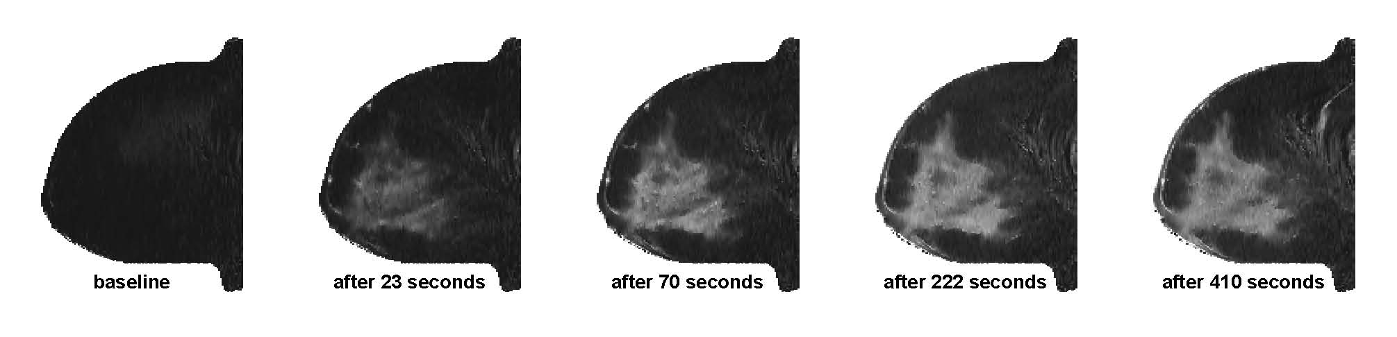
Figure 1: Time series of contrast concentration images at baseline and after 23, 70, 222 and 410 seconds - central slice from first scan of patient 9.

To validate the proposed methods, the first simulation study evaluates the fit of the semi-parametric technique to simulated data in comparison to a parametric method. The second simulation study evaluates the estimation algorithm for the onset of the enhancement and the kinetic parameters when the arrival of tracer in the tissue ROI is lagged. For in-vivo validation, clinical data of 24 DCE-MRI scans of breast cancer patients were analyzed. A series of dynamic images from a patient is depicted in Fig. 1.

III-A Simulation studies

The semi-parametric technique provides an accurate fit to the observed contrast agent concentration time curve. The sum of the squared residuals (SSR) for the simulated data has a range of $1.89\cdot 10^{-4}$ to $2.13\cdot 10^{-3}$ with a mean of $1.13\cdot 10^{-3}$ over all the 13 experiments. With the reference parametric model, the SSR has a range of $0.198$ to $1.520$ with a mean of $0.661$, i.e., the fit to the observed data was poor in the reference parametric model compared to the proposed semi-parametric technique.

Fig. 2 depicts the the kinetic parameter estimates for the semi-parametric technique and the reference parametric method compared to the ground truth. Fig. 2 (a) shows that the parameter $K^{\text{trans}}$ is underestimated with the reference parametric model – on average by 17.7%, which is consistent with previously published results [6]. By contrast, $K^{\text{trans}}$ estimates with the semi-parametric technique are much closer to the ground truth. The mean deviation from the ground truth is 6.2%. These results suggest that the semi-parametric technique is more stable compared to the parametric model.changes in $v_{p}$.

With the proposed semi-parametric technique, the parameters $k_{\text{ep}}$ and $v_{p}$ are also estimated accurately, but $k_{\text{ep}}$ is slightly overestimated by 1.5% to 6.2% compared to a strong overestimation of 39% to 100% with the reference parametric method. For most experiments, the $v_{p}$ parameter obtained from the semi-parametric technique is much closer to the ground truth than that of the the reference model. For small values of $v_{p}$ (experiment 6), however, the semi-parametric method shows a larger deviation from ground truth. An important advantage of the proposed Bayesian technique is that it not only produces point estimates, but also estimations of the errors or interval estimators. Tab. II gives 95% Credible Intervals (CI) for $K^{\text{trans}}$ for all the 13 experiments conducted. For experiments 8 and 9, where $v_{p}$ has larger values, the 95% CI are broad, but still cover the true value. Similar CIs are available for the other parameters. The Bayesian technique provides important information about both the accuracy and precision of its estimates.

To validate the proposed algorithm for estimating the onset of the contrast uptake, a time lag of up to 30 seconds was added to the down-sampled simulated data. Data was analyzed with the proposed semi-parametric technique and the enhancement onset time and the kinetic parameters were derived by equations described in section II-C. The estimation of $t_{0}$ with the proposed method is shown to be accurate. Correlation between the estimated onset time and ground truth is $0.9984$. The mean difference between the true and estimated onset time is $0.1800$ seconds with a standard deviation of $0.9339$ seconds and a maximum absolute difference of $2.2992$ seconds.

Fig. 3 shows the Mean Absolute Difference (MAD) between the estimated values of $K^{\text{trans}}$ and the ground truth. The MAD is stable with increasing time lag, but changes periodically with respect to the sampling interval of 8 seconds. For comparison, the lagged data was further analyzed without $t_{0}$ estimation. For a small time lag up to 8 seconds, i.e., up to one sampling interval, a lag of the onset time has negligible influence on $K^{\text{trans}}$ estimation. However, for larger onset lags MAD increases significantly when onset is not taken into account.

III-B In vivo validation

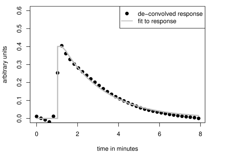
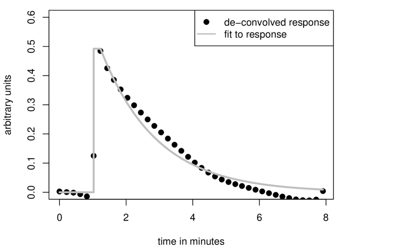
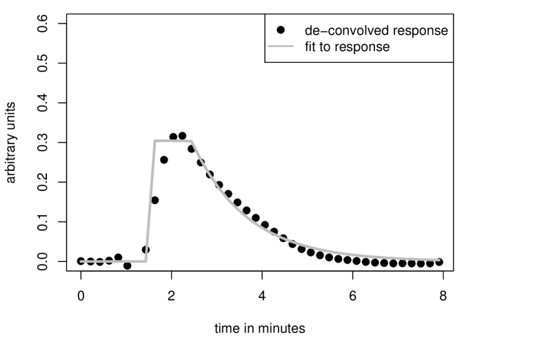
Figure 4: Left column: Observed contrast agent concentration time series (dots) of a voxel in the ROI of the pre-treatment scans for three different subjects (from top to bottom: subjects 5, 9 and 4) along with fit by parametric (slashed line) and semi-parametric technique; for the semi-parametric technique the median (solid line) and the 95% CI (dotted lines) are depicted. The estimated enhancement onset time is marked as vertical line. Right column: Median estimated de-convolved response function (dots) with fit to the model Eqn. 20 (grey line) for the same voxels.

Table III shows the sum of squared residuals (SSR), i.e., the goodness of fit for the data from all 24 in-vivo scans obtained from the semi-parametric and the parametric approach. As with the simulated data, the fit is clearly better for the semi-parametric technique. Table IV provides the estimated enhancement onset time for all scans; the scanning protocol indicates that the contrast agent was injected at the start of the fifth image, i.e. after $49.40s$. For three subjects, the onset time is displayed in Fig. 4 as vertical dashed line. Visual inspection of this figure and of the other subjects shows that the estimated onset time is consistent with the observed contrast concentration time series. For most scans, the estimated onset time is between the start of the fifth acquisition and the start of the sixth acquisition, which is reasonable given the scanning protocol. For some scans, however, the onset time is much larger due to deviation from the scanning protocol.

Figs. 4 depicts the observed contrast concentration time series for three voxels from three different scans together with the estimates from the parametric reference method and those from the proposed semi-parametric approach with 95% CI. It is evident that in all voxels the semi-parametric method fits the data better than the parametric approach. The figures also indicate that the standard parametric model is not always appropriate for the observed data, where the initial upslope is difficult to follow by using the parametric model. The model also fails when the assumed onset time strongly deviates from the observed onset time, for example for the first scan of subject 4 (see bottom row of Fig. 4).

In this study, the 95% CI of the contrast agent concentration time series nicely covers the observed CTC. About half the observed points, however, lie outside the CI. The estimated observation error is larger than the estimated error of the CTC, i.e., the uncertainty of the model about the true CTC. For the first scan of subject 4, the CI is noticeably wider than that of other scans, i.e., the quality of the data from this scan is lower than the quality of the other scan. Typically, the CI is wider after the upslope of the CTC, and narrow during wash-out. It widens again at the end of the time series, because the spline fit at the end point relies on less data.

Fig. 4 also depicts the median of the estimated de-convolved response function and the fit to the parametric model Eqn. 20 for the same three voxels. Although there is no restriction on the form of the response function, the estimated response always has the expected shape: start at zero, rapid upslope, a short plateau and a nearly exponential downslope. The response function is well characterized by using Eqn. 20, and gives robust estimates of the kinetic parameters across the given ROI. However, the first part of the response function is typically slightly underestimated and the second part is slightly overestimated. A more flexible parametric model might fit the response function better.

	Patient 2	Patient 3	Patient 9
SSR parametric
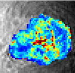
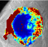
SSR semi-parametric
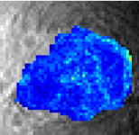
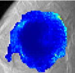
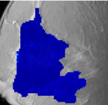
$K^{\text{trans}}$ parametric
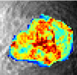
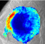
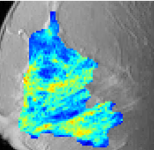
$K^{\text{trans}}$ semi-parametric
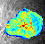
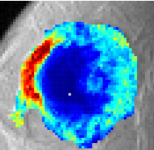
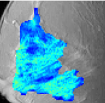
standard error $K^{\text{trans}}$

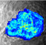
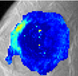
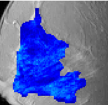
Figure 5: Parameter maps for the first scan of patients 2, 3 and 9. From top to bottom: Sum of squared residuals (SSR) map for reference parametric technique; SSR map for proposed semi-parametric technique; $K^{\text{trans}}$ parameter map estimated with reference parametric technique; $K^{\text{trans}}$ parameter map estimated with proposed semi-parametric technique standard error of $K^{\text{trans}}$ estimated from proposed semi-parametric technique.

Fig. 5 (rows 1 and 2) depicts the sum of squared residuals (SSR) in the ROI for the semi-parametric technique and the reference parametric method for the pre-treatment scans of three patients. SSRs are clearly reduced over the whole area of the tumor, especially in areas with high $K^{\text{trans}}$ values, i.e., in areas with fast blood flow. Therefore, $K^{\text{trans}}$ estimates are clearly different for both methods, parameter maps are shown in Fig. 5 (row 3 and 4). There is, however, no general trend for under- or overestimation with different methods. For example, for subject 9, $K^{\text{trans}}$ estimates are higher with the parametric method, as the upslope is overestimated (see also Fig. 4). On the other hand, for patient 3, $K^{\text{trans}}$ estimates are to low by using the parametric technique due to a wrong onset time. Again, the Bayesian method allows us to access the precision of the estimated kinetic parameters. Fig. 5 (row 5) depicts the standard error of the $K^{\text{trans}}$ parameter computed with the semi-parametric technique. Estimation errors are higher with higher values, but they are generally relatively small. For most voxels, the relative error, i.e., standard error divided by estimated parameter, does not exceed 20%.

IV Conclusion

In this paper, we have introduced a semi-parametric technique based on Bayesian P-spline models for quantifying CTCs obtained with DCE-MRI. Compared with parametric models, the proposed semi-parametric technique provides a superior fit to the observed concentration time curves. In particular, the proposed semi-parametric method captures the upslope of the time series accurately, which is important for an accurate fit of the CTCs in DCE-MRI and proper calculation of $K^{\text{trans}}$.

Results from the simulated data show a clear improvement in both time curve fit and parameter estimation. In addition, the Bayesian method provides information about the precision of the estimation, including standard errors or credible intervals. For in vivo validation, the fit of the contrast agent concentration with the proposed semi-parametric technique is superior to the parametric method. Estimates of kinetic parameters for both techniques are different where the fit of the parametric technique is poor, suggesting that the estimation of kinetic parameters with the proposed semi-parametric technique is more accurate in these areas. The exact assessment of the kinetics is clinically important as changes in respect to the response function and the kinetic parameters can be subtle, especially for drugs that cause multiple effect on tumor vasculature, such as combinations of antiangiogenic drugs [34].

Non-linear parametric models are typically difficult to estimate due to the convergence issues and problems in specifying consistent starting values. Bayesian non-linear regression can overcome these convergence problems, but at a cost of computational time [14]. The proposed semi-parametric method provides a reliable and practical way of circumventing these problems. With the proposed technique, computation only includes sampling from standard distributions (see section II-B4) which can be done efficiently [35] and gives good mixing of the MCMC kernel.

In contrast to classical approaches [12], Bayesian P-splines allow simultaneous estimation of model and smoothing parameters. Adaptive smoothing parameters can be obtained and are important to model the sharp changes in the dynamic series of the contrast concentration.

One unique feature of the paper is the estimation of the onset of the CTC based on Bayesian inference. Onset time can be determined for the whole region of interest or on a more local level. It is an important parameter in quantitative DCE-MRI models as it has great influence on other parameters in the kinetic model and an incorrect onset time can lead to a strong bias in parameter estimates [15]. Onset time is also an important clinical index for characterizing suspicious breast lesions [36], although in this study they are not evident for the patients studied.

The proposed method allows a direct assessment of the response function, i.e., the actual flow in the tissue. Parameters of interest may be estimated by fitting a non-linear model to the response function. Smoothing via P-splines provides an effective way of error reduction and deconvolution of the arterial input function. The proposed technique also allows the quantification of errors both in fitting the observed data and in estimating kinetic parameters. Thus far, the estimation error in DCE-MRI models is rarely discussed, the proposed technique can contribute to the evaluation of the quality of DCE-MRI scans. Results from the semi-parametric technique can therefore serve as a supporting tool for quality control. When choosing a pixel, the CTC would be displayed interactively along with the semi-parametric fit, the CI, and the estimated onset time. This would not only help to reassess the quality of the data, but also make it easier to understand what is actually happening physiologically.

TABLE I: Values of the kinetic parameters describing the behavior of MMID4 used to simulate 13 different contrast concentration time curves representative of a breast tumor.

Exp.	Baseline	2	3	4	5	6	7	8	9	10	11	12	13
$F_{p}$	0.57	0.17	0.37	0.77	0.97	0.57				0.57
$v_{p}$	0.06	0.06				$10^{-4}$	0.03	0.09	0.12	0.06
$PS$	0.33	0.33				0.33				0.01	0.17	0.49	0.65
$v_{e}$	0.45	0.45				0.45				0.45

TABLE II: True and estimated values of $K^{\text{trans}}$ with 95% CI.

Experiment	1	2	3	4	5	6	7	8	9	10	11	12	13
True $K^{\text{trans}}$	0.251	0.146	0.218	0.268	0.280	0.233	0.233	0.233	0.233	0.010	0.147	0.323	0.388
2.5% quantile $K^{\text{trans}}$	0.208	0.128	0.201	0.236	0.242	0.181	0.220	0.224	0.229	0.004	0.129	0.293	0.347
Median posterior $K^{\text{trans}}$	0.245	0.138	0.218	0.263	0.284	0.200	0.237	0.281	0.282	0.005	0.147	0.320	0.376
97.5% quantile $K^{\text{trans}}$	0.267	0.167	0.240	0.309	0.376	0.239	0.256	0.334	0.372	0.060	0.183	0.356	0.415

TABLE III: Sum of squared residuals (SSR) between data and fitted function for parametric and semi-parametric method, averaged over all voxels in the ROI.

1st scan, subject	1	2	3	4	5	6
parametric	0.0682	0.1579	0.2209	0.1825	0.6101	0.4382
semi-parametric	0.0217	0.0575	0.0341	0.183	0.0398	0.0333
	7	8	9	10	11	12
parametric	0.0723	0.0366	0.0798	0.0568	0.1420	0.0552
semi-parametric	0.0242	0.0068	0.104	0.0077	0.0131	0.0234
2nd scan, subject	1	2	3	4	5	6
parametric	0.0457	0.0691	0.0403	0.8665	0.6469	0.5804
semi-parametric	0.0123	0.0328	0.0122	0.0484	0.0386	0.0334
	7	8	9	10	11	12
parametric	0.0998	0.0525	0.0237	0.0544	0.0225	0.0289
semi-parametric	0.0209	0.0102	0.0071	0.0205	0.0072	0.0168

TABLE IV: Estimated contrast concentration enhancement onset time in seconds for all 24 scans. Protocol specified that the tracer was injected after 49.40 seconds.

Subject	1	2	3	4	5	6	7	8	9	10	11	12
1st scan	55.19	54.14	69.09	90.20	60.04	57.63	52.56	54.95	55.85	56.72	47.48	50.34
2nd scan	55.09	56.58	87.09	56.58	56.71	55.31	53.10	55.46	53.33	53.96	54.06	49.59

Figure 2: Scatter plots of parameter estimates vs. true values – These figures are similar to Fig. 3 in [6]. Estimates of the parameters (a) $K^{\text{trans}}$, (b) $k_{\text{ep}}$ and (c) $v_{p}$. Bullets represent the results using the semi-parametric method, diamonds the results using the parametric technique.

Figure 3: Mean absolute difference between true and estimated $K^{\text{trans}}$ values plotted against true enhancement onset time in seconds. Solid dots are results from semi-parametric analysis without considering onset, circles are results from the proposed algorithm with onset estimation.

References

- [1] V. J. Schmid, B. Whitcher, and G. Z. Yang, “Semi-parametric analysis of dynamic contrast-enhanced MRI using Bayesian P-splines,” in Medical Imaging Computing and Computer-Assisted Intervention – MICCAI 2006, ser. Lecture Notes in Computer Science, R. Larsen, M. Nielsen, and J. Sporring, Eds., no. 4190. Berlin: Springer, 2006, pp. 679–686.
- [2] D. J. Collins and A. R. Padhani, “Dynamic magnetic resonance imaging of tumor perfusion,” IEEE Engineering in Biology and Medicine, vol. 23, no. 5, pp. 65–83, Sep-Oct 2004.
- [3] G. J. M. Parker and A. R. Padhani, “-w DCE-MRI: -weighted dynamic contrast-enhanced MRI,” in Quantitative MRI of the Brain, P. Tofts, Ed. Chichester, England: Wiley, 2003, ch. 10, pp. 341–364.
- [4] E. K. Fram, R. J. Herfkens, G. A. Johnson, G. H. Glover, J. P. Karis, A. Shimakawa, T. G. Perkins, and N. J. Pelc, “Rapid calculation of T1 using variable flip angle gradient refocused imaging,” Magnetic Resonance Imaging, vol. 5, pp. 201–208, 1987.
- [5] H. B. Larsson and P. S. Tofts, “Measurement of the blood-brain barrier permeability and leakage space using dynamic Gd-DTPA scanning – a comparison of methods,” Magnetic Resonance in Medicine, vol. 24, no. 1, pp. 174–176, 1992.
- [6] D. L. Buckley, “Uncertainty in the analysis of tracer kinetics using dynamic contrast-enhanced -weighted MRI,” Magnetic Resonance in Medicine, vol. 47, no. 3, pp. 601–606, 2002.
- [7] K. S. St.Lawrence and T.-Y. Lee, “An adiabatic approximation to the tissue homogeneity model for water exchange in the brain: I. theoretical derivation,” Journal of Cerebral Blood Flow & Metabolism, vol. 18, pp. 1365–1377, 1998.
- [8] T. Twellmann, O. Lichte, and T. W. Nattkemper, “An adaptive tissue characterization network for model-free visualization of dynamic contrast-enhanced magnetic resonance image data,” IEEE Transactions on Medical Imaging, vol. 24, no. 10, pp. 1256–66, October 2005.
- [9] K.-H. Chaung, M.-T. Wu, Y.-R. Lin, K.-S. Hsieh, M.-L. Wu, S.-Y. Tsai, C.-W. Ko, and H.-W. Chung, “Application of model-free analysis in the MR assessment of pulmonary perfusion dynamics,” Magnetic Resonance in Medicine, vol. 54, no. 2, pp. 299–308, 2005.
- [10] V. J. Cunningham and T. Jones, “Spectral analysis of dynamic PET studies,” Journal of Cerebral Blood Flow and Metabolism, vol. 13, pp. 15–23, 1993.
- [11] R. N. Gunn, S. R. Gunn, F. E. Turkheimer, J. A. D. Aston, and V. J. Cunningham, “Positron emission tomography compartmental models: A basis pursuit strategy for kinetic modeling,” Journal of Cerebral Blood Flow and Metabolism, vol. 22, pp. 1425–1439, 2002.
- [12] M. Jerosch-Herold, C. Swingen, and R. Seethamraju, “Myocardial blood flow quantification with MRI by model-independent deconvolution,” Medical Physics, vol. 29, no. 5, pp. 886–897, May 2002.
- [13] C. Gössl, L. Fahrmeir, and D. P. Auer, “Bayesian modeling of the hemodynamic response function in BOLD fMRI,” NeuroImage, vol. 14, pp. 140–148, 2001.
- [14] V. J. Schmid, B. Whitcher, G. Z. Yang, N. J. Taylor, and A. R. Padhani, “Statistical analysis of pharmacokinetical models in dynamic contrast-enhanced magnetic resonance imaging,” in Medical Imaging Computing and Computer-Assisted Intervention – MICCAI 2005, ser. Lecture Notes in Computer Science, J. Duncan and G. Gerig, Eds., no. 3750. Berlin: Springer, 2005, pp. 886–893.
- [15] M. R. Orton, D. J. Collins, S. Walker-Samuel, J. A. d’Arcy, D. J. Hawkes, D. Atkinson, and M. O Leach, “Bayesian estimation of pharmacokinetic parameters for DCE-MRI with a robust treatment of enhancement onset time,” Physics in Medicine and Biology, vol. 52, pp. 2393–2408, 2007.
- [16] V. J. Schmid, B. Whitcher, A. R. Padhani, N. J. Taylor, and G.-Z. Yang, “Bayesian methods for pharmacokinetic models in dynamic contrast-enhanced magnetic resonance imaging,” IEEE Transactions on Medical Imaging, vol. 25, no. 12, pp. 1627–1636, December 2006.
- [17] P. Eilers and B. Marx, “Flexible smoothing with B-splines and penalties (with comments and rejoinder),” Statistical Science, vol. 11, no. 2, pp. 89–121, 1996.
- [18] B. Marx and P. Eilers, “Direct generalized additive modeling with penalized likelihood,” Computational Statistics and Data Analysis, vol. 28, no. 2, pp. 193–209, 1998.
- [19] P. R. Johnston and R. M. Gulrajani, “Selecting the corner in the L-curve approach to Tikhonov regularization,” IEEE Transaction on Biomedical Engineering, vol. 47, p. 1293, Sept. 2000.
- [20] S. Lang, E. Fronk, and L. Fahrmeir, “Function estimation with locally adaptive dynamic models,” Computational Statistics, vol. 17, pp. 479–500, 2002.
- [21] S. Lang and A. Brezger, “Bayesian P-splines,” Journal of Computational and Graphical Statistics, vol. 13, pp. 183–212, 2004.
- [22] S. Kety, “Blood-tissue exchange methods. Theory of blood-tissue exchange and its applications to measurement of blood flow.” Methods in Medical Research, vol. 8, pp. 223–227, 1960.
- [23] P. S. Tofts, G. Brix, D. L. Buckley, J. L. Evelhoch, E. Henderson, M. V. Knopp, H. B. W. Larsson, T.-Y. Lee, N. A. Mayr, G. J. M. Parker, R. E. Port, J. Taylor, and R. Weiskoff, “Estimating kinetic parameters from dynamic contrast-enhanced -weighted MRI of a diffusable tracer: Standardized quantities and symbols,” Journal of Magnetic Resonance Imaging, vol. 10, pp. 223–232, 1999.
- [24] P. Tofts and A. Kermode, “Measurement of the blood-brain barrier permeability and leakage space using dynamic MR imaging – 1. Fundamental concepts,” Magnetic Resonance in Medicine, vol. 17, pp. 357–367, 1991.
- [25] T. Fritz-Hansen, E. Rostrup, K. B. Larsson, L. Søndergaard, P. Ring, and O. Henriksen, “Measurement of the arterial concentration of Gd-DTPA using MRI: A step toward quantitative perfusion imaging,” Magnetic Resonance in Medicine, vol. 36, pp. 225–231, 1996.
- [26] J. J. Moré, “The Levenberg-Marquardt algorithm: Implementation and theory,” in Numerical Analysis: Proceedings of the Biennial Conference held at Dundee, June 28-July 1, 1977 (Lecture Notes in Mathematics #630), G. A. Watson, Ed. Berlin: Springer-Verlag, 1978, pp. 104–116.
- [27] K. Kroll, N. Wilke, M. Jerosch-Herold, Y. Wang, Y. Zhang, R. J. Bache, and J. B. Gassingthwaighte, “Modeling regional myocardial flows from residue functions of an intravascular indicator,” American Journal of Heart Circulation Physiology, vol. 271, pp. 1643–1655, 1996.
- [28] C. Landis, X. Li, F. W. Telang, J. A. Coderre, P. L. Micca, W. D. Rooney, L. L. Latour, G. Vétek, I. Pályka, and C. S. Springer, “Determination of the MRI contrast agent concentration time course in vivo following bolus injection: Effect of equilibrium transcytolemmal water exchange,” Magnetic Resonance in Medicine, vol. 44, pp. 567–574, 2000.
- [29] W. R. Gilks, S. Richardson, and D. J. Spiegelhalter, Eds., Markov Chain Monte Carlo in Practice. Chapman & Hall, London, 1996.
- [30] M. Jerosch-Herold, X. Hu, N. Murthy, and R. Seethamraju, “Time delay for arrival of MR contrast agent in collateral-dependent myocardium,” IEEE Transactions on Medical Imaging, vol. 23, no. 7, pp. 881–890, July 2004.
- [31] N.-K. Tsao and T.-C. Sun, “On the numerical computation of the derivatives of a B-spline series,” IMA Journal of Numerical Analysis, vol. 13, no. 3, pp. 343–364, 1993.
- [32] M. O. Leach, K. M. Brindle, J. L. Evelhoch, J. R. Griffiths, M. R. Horsman, A. Jackson, G. C. Jayson, I. R. Judson, M. V. Knopp, R. J. Maxwell, D. McIntyre, A. R. Padhani, P. Price, R. Rathbone, G. J. Rustin, P. S. Tofts, G. M. Tozer, W. Vennart, J. C. Waterton, S. R. Williams, and P. Workman, “The assessment of antiangiogenic and antivascular therapies in early-stage clinical trials using magnetic resonance imaging: issues and recommendations,” British Journal of Cancer, vol. 92, pp. 1599–1610, 2005.
- [33] M.-L. W. Ah-See, A. Makris, N. J. Taylor, R. J. Burcombe, M. Harrison, J. J. Stirling, P. I. Richman, M. O. Leach, and A. R. Padhani, “Does vascular imaging with MRI predict response to neoadjuvant chemotherapy in primary breast cancer?” Journal of Clinical Oncology (Meeting Abstracts), vol. 22, no. 14S, p. 582, 2004.
- [34] A. R. Padhani and M. O. Leach, “Antivascular cancer treatments: functional assessments by dynamic contrast-enhanced magnetic resonance imaging,” Abdominal Imaging, vol. 30, no. 3, pp. 325–342, 2005.
- [35] H. Rue, “Fast sampling of Gaussian Markov random fields,” Journal of the Royal Statistical Society Series B, vol. 63, pp. 325–338, 2001.
- [36] C. Boetes, J. Barentsz, R. Mus, R. van der Sluis, L. van Erning, J. Hendriks, R. Holland, and S. Ruys, “MR characterization of suspicious breast lesions with a gadolinium-enhanced TurboFLASH subtraction technique,” Radiology, vol. 193, no. 3, pp. 777–781, 1994.