Geometrically controllable electric fields

Abstract

According to a first-principles approach, we clarify electric cloaks’ universality concerning a new class of phase transitions between negative pathway (NGP) and normal pathway of electric displacement fields, which are driven by the geometric shape of the cloak. We report that the NGP arises from shape-enhanced strong negative electric polarization, and that it is related to a symmetric oscillation of the paired electric permittivities, which are shown to satisfy a sum rule. The NGP does not occur for a spherical cloak, but appears up to maximum as the ratio $a/b$ between the long- and short- principal axis of the spheroidal cloak is about 5/2, and eventually disappears as $a/b$ becomes large enough corresponding to a rod-like shape. Then, the cloaking efficiency is compared between different geometrical shapes. The possibility of experiments is discussed. This work has relevance to crucial control of electric fields and to general physics of phase transitions.

1 Introduction

Metamaterials VeselagoSP68 ; PendryPRL96 are a new class of electromagnetic materials, which are currently under extensive investigation SmithS04 ; PendryS06 ; SchurigOE06 ; SchurigS06 ; RuanPRL07 ; YanPRL07 ; ChenPRL07 ; CaiNP07 . They owe their properties to subwavelength details of structure rather than to their chemical composition, and can be designed to have properties difficult or impossible to find in nature. An electromagnetic spherical cloak is well-known for hiding objects from electro-magnetic waves PendryS06 ; SchurigOE06 ; SchurigS06 ; CaiNP07 , due to the high freedom of design of metamaterials SmithS04 , which may be both inhomogeneous and anisotropic in their electric permittivity and magnetic permeability SmithS04 ; PendryS06 ; SchurigOE06 ; SchurigS06 ; RuanPRL07 ; YanPRL07 ; ChenPRL07 . Owing to intriguing potential applications, it has received extensive attention, e.g., ranging from its two-dimensional counterpart SchurigOE06 ; RuanPRL07 ; YanPRL07 and scattering cross section ChenPRL07 , to its extensions like acoustic cloaks ChenAPL07 . In this work, by using a first-principles approach based on the coordinate transformation method, we investigate electric cloaks and clarify their universality concerning a new class of phase transition between negative pathway (NGP) and normal pathway (NMP) of electric displacement fields as geometric shape of the cloak changes in a typical range. The shape-driven phase transition seems to be of particular interest when compared with abundant phase transitions already known in condensed matter and nature. We shall also calculate cloaking efficiency of the electric cloaks with various shapes. This work has relevance to crucial control of electric fields and to general physics of phase transitions.

The remainder of this work is organized as follows. In Section 2, based on the coordinate transformation method, we present a first-principles approach to derive the expressions for electric permittivities in electric cloaks with non-spherical shapes. This is followed by Section 3, in which we numerically clarify their universality concerning the phase transition between negative pathway and normal pathway of electric displacement fields, and calculate cloaking efficiency under various conditions. This paper ends with a discussion and conclusion in Section 4.

2 Formalism

To proceed, we shall use a first-principles approach, namely, the coordinate transformation method PendryS06 ; SchurigOE06 . We consider that each point in the original Cartesian coordinates can be represented as $(x,y,z)$, while in the distorted coordinates it can be given as $(u,v,w)$, which is the location of the new point with respect to the $x$, $y$, and $z$ axes, namely, $u=u(x,y,z)$, $v=v(x,y,z)$, and $w=w(x,y,z)$ PendryS06 . In the distorted coordinates, the form of Maxwell’s Equations are invariant, but the corresponding electric permittivity are got in the following form $\epsilon_{u}^{\prime}=\epsilon_{u}\frac{Q_{u}Q_{v}Q_{w}}{Q_{u}^{2}}$ ($\epsilon_{u}$: electric permittivity in the original Cartesian coordinates), where

$$Q_{u}^{2} = \left(\frac{\partial x}{\partial u}\right)^{2}+\left(\frac{\partial y}{\partial u}\right)^{2}+\left(\frac{\partial z}{\partial u}\right)^{2},$$ (1)

$$Q_{v}^{2} = \left(\frac{\partial x}{\partial v}\right)^{2}+\left(\frac{\partial y}{\partial v}\right)^{2}+\left(\frac{\partial z}{\partial v}\right)^{2},$$ (2)

$$Q_{w}^{2} = \left(\frac{\partial x}{\partial w}\right)^{2}+\left(\frac{\partial y}{\partial w}\right)^{2}+\left(\frac{\partial z}{\partial w}\right)^{2}.$$ (3)

Now we consider an ellipsoidal cloak in three dimensions. In the Cartesian coordinates $(x,y,z)$, the equation for describing an ellipsoidal shape is

$$\frac{x^{2}}{a^{2}}+\frac{y^{2}}{b^{2}}+\frac{z^{2}}{c^{2}}=1,$$

where $a$, $b$, and $c$ are the three principal semi-axes of the ellipsoid, respectively. Next, we choose $(\lambda,\mu,\nu)$ to represent a point in the ellipsoidal coordinates. So far, the relation between $(\lambda,\mu,\nu)$ and $(x,y,z)$ is given as

$$x^{2} = \frac{\left(a^{2}+\lambda\right)\left(a^{2}+\mu\right)\left(a^{2}+\nu\right)}{\left(a^{2}-b^{2}\right)\left(a^{2}-c^{2}\right)},$$ (4)

$$y^{2} = \frac{\left(b^{2}+\lambda\right)\left(b^{2}+\mu\right)\left(b^{2}+\nu\right)}{\left(b^{2}-c^{2}\right)\left(b^{2}-a^{2}\right)},$$ (5)

$$z^{2} = \frac{\left(c^{2}+\lambda\right)\left(c^{2}+\mu\right)\left(c^{2}+\nu\right)}{\left(c^{2}-a^{2}\right)\left(c^{2}-b^{2}\right)}.$$ (6)

Then, we squeeze the ellipsoidal volume into an ellipsoidal shell through the following relations

$$\lambda^{\prime} = a_{1}+\lambda\frac{a_{2}-a_{1}}{a_{2}},$$ (7)

$$\mu^{\prime} = b_{1}+\mu\frac{b_{2}-b_{1}}{b_{2}},$$ (8)

$$\nu^{\prime} = c_{1}+\nu\frac{c_{2}-c_{1}}{c_{2}},$$ (9)

where $a_{1}$, $b_{1}$, and $c_{1}$ ($a_{2}$, $b_{2}$, and $c_{2}$) are the inner (outer) three principal semi-axes of the ellipsoidal shell. In the distorted ellipsoidal coordinates, we have the renormalized values of electric permittivities, $\epsilon_{\lambda^{\prime}}^{\prime}$, $\epsilon_{\mu^{\prime}}^{\prime}$, and $\epsilon_{\nu^{\prime}}^{\prime}$, inside the ellisoidal cloak (shell):

$$\epsilon_{\lambda^{\prime}}^{\prime} = \frac{a_{2}}{a_{2}-a_{1}}\frac{b_{2}}{b_{2}-b_{1}}\frac{c_{2}}{c_{2}-c_{1}}\frac{(\lambda^{\prime}-a_{1})^{2}}{\lambda^{\prime 2}}\epsilon_{host},$$ (10)

$$\epsilon_{\mu^{\prime}}^{\prime} = \frac{a_{2}}{a_{2}-a_{1}}\frac{b_{2}}{b_{2}-b_{1}}\frac{c_{2}}{c_{2}-c_{1}}\frac{(\mu^{\prime}-b_{1})^{2}}{\mu^{\prime 2}}\epsilon_{host},$$ (11)

$$\epsilon_{\nu^{\prime}}^{\prime} = \frac{a_{2}}{a_{2}-a_{1}}\frac{b_{2}}{b_{2}-b_{1}}\frac{c_{2}}{c_{2}-c_{1}}\frac{(\nu^{\prime}-c_{1})^{2}}{\nu^{\prime 2}}\epsilon_{host},$$ (12)

where $\epsilon_{host}$ denotes the electric permittivity outside the cloak. From equations (10)-(12), we can see that the electric permittivities are both materially anisotropic and spatially inhomegeneous in the distorted ellipsoidal coordinates. For achieving them, metamaterials can help SmithS04 .

3 Numerical results

3.1 Phase transition between negative pathway and normal pathway of electric displacement fields

In our numerical simulations, there are three domains in the whole system, namely, the inner domain (domain I), the cloaking or shell domain (domain II), and the outer domain (domain III). For convenience, we set the electric permittivity of domain I to have the same value as that $\epsilon_{host}$ of domain III, and further take $\epsilon_{host}$ to be equal to the electric permittivity of free space $\epsilon_{0}$. This will not affect our results at all because the main interest of this work is on geometrical control of electric fields within domain II. The electric permittivity of domain II is determined according to equations (10)-(12). For all the spherical or non-spherical cloaks discussed in Figs. 1-5, we keep the volume ratio between domain II and domain I at 7:1, and the applied electric potentials are set to be +3 V and -3 V at the two opposite planes of the cubic box, respectively. It is worth mentioning that our results are independent of the actual value of the potentials. As the spherical cloak is centro-symmetric, it makes no difference when the electric field is applied in various directions. However, for an ellipsoidal cloak, we have to discriminate the direction of applied electric fields due to the existence of geometric anisotropy. In our simulations, we apply the electric potentials in two opposite planes along the three principal axes, $a$, $b$, and $c$, of the ellipsoidal cloak, respectively. We focus on two types of rotational ellipsoid (namely, spheroid) with $a<b=c$ (oblate spheroid) and $a>b=c$ (prolate spheroid). Throughout this work, the set of $a,b,$ and $c$ will be used to denote both three inner principal semi-axes ($a_{1}$, $b_{1}$, and $c_{1}$) and three outer principal semi-axes ($a_{2}$, $b_{2}$, and $c_{2}$) of the ellipsoidal cloak if there are no special instructions. We should also remark that our simulation results are independent of the length scale of the electric cloaks.

The streamlines of Fig. 1 represent the pathway of the electric displacement field in the electric spherical cloak for the parameters as indicated in the caption. Clearly, the displacement field goes around the inner domain, but is limited within the cloak (shell), and eventually returns to its original pathway. In this process, an object inside the inner domain has no effect on the displacement field at all. In other words, the object is protected from the invasion of electric fields by using the electric cloak. (Its cloaking efficiency will further be investigated in Section 3.2.)

For a spheroidal cloak, the pathway of the electric displacement field is also illustrated in Fig. 2 (oblate spheroid) and Fig. 3 (prolate spheroid). For the oblate spheroidal cloak $a<b=c$, the pathway is similar to the spherical cloak discussed in Fig. 1 when the applied electric field is directed along the short principal semi-axis $a$, see Fig. 2. However, the situation becomes different for the case of prolate spheroid with $a>b=c$, as shown in Fig. 3 in which the external electric field is along the long principal semi-axis $a$. Figure 3 shows a NGP (negative pathway) of the electric displacement field inside the spheroidal cloak. Here, the so-called NGP means that the displacement field goes backwards, in contrast to NMP (normal pathway) for which the field goes forwards. (All the NGP streamlines shown in Fig. 3 are seemingly limited to enter the inner domain. However, this is actually not true. Depending on different streamlines/pathways and/or shape parameters, such NGP streamlines can also appear within the cloak domain only.) Owing to the symmetry of the prolate spheroid, the NGP zone is strictly symmetrical, which locates close to the two opposite sides of the prolate cloak. On the other hand, we have also investigated the case of a general ellipsoid with $a\neq b\neq c$ for which the external electric field is directed along the longest principal semi-axis, the behavior is generally similar to Fig. 3 (no figures shown here). Nevertheless, in this case, the NGP zone is no longer strictly symmetrical, the degree of which depends on the actual values of $a$, $b$, and $c$.

Now let us dig out the physical origin of the NGP mentioned above. It is known that an electric displacement field ${\bf D}$ is given by ${\bf D}=\epsilon_{0}{\bf E}+{\bf P},$ where ${\bf E}$ is the external electric field, and $P$ an electric polarization. Corresponding to the NGP, ${\bf D}$ has a negative sign, which is opposite to ${\bf E}$ (Strictly, there is an obtuse angle between ${\bf D}$ and ${\bf E}$ in the present case, due to the presence of anisotropic and inhomogeneous electric permittivities inside the cloak). Thus, this requires that ${\bf P}$ should be sufficiently negative, satisfying ${\bf P}<-\epsilon_{0}{\bf E}$. So far, we can conclude that the appearance of the NGP zone results from the shape-enhanced strong negative electric polarization.

Figure 4(a) shows a phase diagram for spheroidal cloak with three principal semi-axes $a\neq b=c$, in the presence of external electric fields along the direction of the principal semi-axis $a$. For this phase diagram, the potential difference $U_{AB}$ (see the caption for its definition) is taken to be the order parameter, and the ratio between $a$ and $b$ ($a:b$) the tuning parameter ranging from 0 to 3.6. In the typical region of $a:b$, a phase transition phenomenon comes to appear. In detail, there is an existence of two distinct phases, NMP phase and NGP phase, and a transition region between them, in which the NGP is enhanced significantly. Such a phase transition is driven by geometrical shape of the cloak. To understand more clearly, in Fig. 4(b) we investigate $U_{AB}$ as a function of $a:b$ ranging from 0 to 20. It is evident that when $a:b$ is smaller than or equal to 1 (oblate spheroid or sphere), the electric potential $U_{AB}=0$, namely, there is no NGP. As $a:b>1$ (prolate spheroid), the NGP comes to appear, and reach maximum at about $a:b=5:2$. Eventually, it tends to disappear as $a:b$ is large enough corresponding to a rod-like shape.

Figure 5 illustrates the paired electric permittivities, $\epsilon_{\lambda}$ and $\epsilon_{\mu}$, in the NGP streamline within the cross section of the spheroidal cloak with $a>b=c$ as a function of the distance $r$ (see the caption), for $a:b=$ (a) $2:1$, (b) $3:1$, and (c) $4:1$. All the points displayed in (a)-(c) have been taken in sequence from the starting point to the ending point of the NGP streamline, as indicated by the ordered numbers. As $a:b$ is given, all the paired $\varepsilon_{\lambda}$ and $\varepsilon_{\mu}$ (corresponding to the same number) appear in a symmetric oscillation trajectory, and satisfy a sum rule: (a) $\varepsilon_{\lambda}+\varepsilon_{\mu}=2.015\pm 0.003$, (b) $2.218\pm 0.007$, and (c) $2.461\pm 0.006$. It is worth noting that the electric permittivity $\varepsilon_{\nu}$ keeps unchanged for the cross section (in two dimensions) of our interest.

3.2 Cloaking efficiency

We define the cloaking efficiency $\eta$ as the total electric energy of domains II and III over the whole system of domains I, II, and III. Apparently, if $\eta$ is equal to 100%, the cloaking is perfect. In this case, any objects within domain I can be perfectly shielded from external electric fields. In other words, the degree of imperfectness of the cloaking is denoted by how $\eta$ deviates from $100\%.$ For consistence, the applied electric potentials and the electric permittivities of domains I, II, and III are set to be the same as those already presented in Section 3.1. In the simulations, the volume ratio between domain II and domain I is also kept at 7:1.

The calculated cloaking efficiencies of the electric cloaks under different conditions are shown in Tables I-III. As we can see, the cloaking efficiency of the spherical cloak is 99.58%, which is very close to, but not equal to 100% (perfect cloaking). The deviation from 100% arises from the small amount of central streamlines that unavoidably pass through domain I. Further, we find that the cloaking efficiencies of non-spherical cloaks are always smaller than that of the spherical cloak. In detail, for prolate spheroidal ($a>b=c$), oblate spheroidal ($a<b=c$), and ellipsoidal ($a\neq b\neq c$) cloaks, their cloaking efficiencies corresponding to three different principal semi-axes have only slight difference and are smaller than that of the spherical cloak. For the three kinds of non-spherical cloaks, we can conclude that the cloaking efficiency corresponding to the field directed along the longest principal semi-axes is the smallest among those along the three principal semi-axes, and that the cloaking efficiency of ellipsoidal ($a\neq b\neq c$) cloaks is the largest whereas that of oblate spheroidal ($a<b=c$) cloaks is the smallest.

4 Discussion and conclusion

Besides DC electric fields adopted in the above simulations, our results also hold for AC fields due to the symmetry of the system. Since they have been obtained by using numerical simulations according to a first-principles approach, namely, the coordinate transformation method, they are exact without any approximation (despite the error which might occur when we extracted the data, e.g., as implied by the sum rules obtained from Fig. 5). Regarding an experimental demonstration, it would be quite convenient to use metamaterials to realize the electric cloaks with a shape-driven phase transition between the NGP and NMP, due to the existing significant achievements in the field SmithS04 ; SchurigS06 . Further, the fact that our results do not depend on specific length-scales makes the experiment more tractable.

To sum up, we have accurately revealed electric cloaks’ universality concerning a new class of shape-driven phase transitions between the NGP and NMP of electric displacement fields. We have showed that the NGP results from shape-enhanced strong negative electric polarization, and that it corresponds to a symmetric oscillation of the paired electric permittivities, which have been demonstrated to satisfy a sum rule. The cloaking efficiency has also been calculated for various geometrical shapes.

We thank W. J. Tian for fruitful discussion. This work was supported by the Pujiang Talent Project (No. 06PJ14006) of the Shanghai Science and Technology Committee, by the Shanghai Education Committee and the Shanghai Education Development Foundation (Shuguang project), by the National Natural Science Foundation of China under Grant No. 10604014, and by Chinese National Key Basic Research Special Fund under Grant No. 2006CB921706.

Figure Captions

Fig. 1. (color online) Spherical cloak (left panel) and its cross section (right panel). The streamlines denote the pathway of the electric displacement field when the applied electric potentials are set to be +3 V and -3 V at the top and bottom plane of the cubic box, respectively. Parameters: $r_{1}=0.1\,$m (inner radius) and $r_{2}=0.2\,$m (outer radius).

Fig. 2. (color online) Oblate spheroidal cloak with three principal semi-axes $a$, $b$, and $c$ satisfying $a<b=c$ (left panel) and its cross section (right panel). The streamlines denote the pathway of the electric displacement field in the direction of the short axis $a$ when the applied electric potentials are set to be +3 V and -3 V at the top and bottom plane of the cubic box. Parameters: $a_{1}=0.1\,$m and $b_{1}=c_{1}=0.2\,$m (three inner principal semi-axes); $a_{2}=0.2\,$m and $b_{2}=c_{2}=0.4\,$m (three outer principal semi-axes).

Fig. 3. (color online) Same as Fig. 2, but for prolate spheroidal cloak $a>b=c$ and the electric displacement field in the direction of the long axis $a$. Parameters: $a_{1}=0.2\,$m and $b_{1}=c_{1}=0.1\,$m; $a_{2}=0.4\,$m and $b_{2}=c_{2}=0.2\,$m.

Fig. 4. (color online) (a) Phase diagram for spheroidal cloak with three principal semi-axes $a\neq b=c$, which represents the existence of two distinct phases, NMP phase and NGP phase, and a transition region between them. The potential difference $U_{AB}$ between the starting point $A$ and ending point $B$ of the NGP streamline [as also indicated in the inset of (b)] is taken to be the order parameter, and the ratio between $a$ and $b$ ($a:b$) the tuning parameter ranging from 0 to 3.6. The three curves correspond to the three incident electric fields, which respectively have a vertical distance of $0.8b$, $0.5b$, and $0.3b$ with respect to the principal semi-axis $a$, see also the inset of (b). (b) $U_{AB}$ as a function of $a:b$ ranging from 0 to 20, and others are the same as (a).

Fig. 5. (color online) The paired electric permittivities, $\epsilon_{\lambda}$ and $\epsilon_{\mu}$, in the NGP streamline within the cross section of the spheroidal cloak with $a>b=c$ as a function of the distance $r$ between any point in the NGP streamline and the center of the cloak, for (a) $a:b=2:1$, (b) $a:b=3:1$, and (c) $a:b=4:1$. All the 20 points have been taken in sequence from the starting point to the ending point of the NGP streamline, as clearly indicated in the corresponding ordered numbers, see also the three insets.

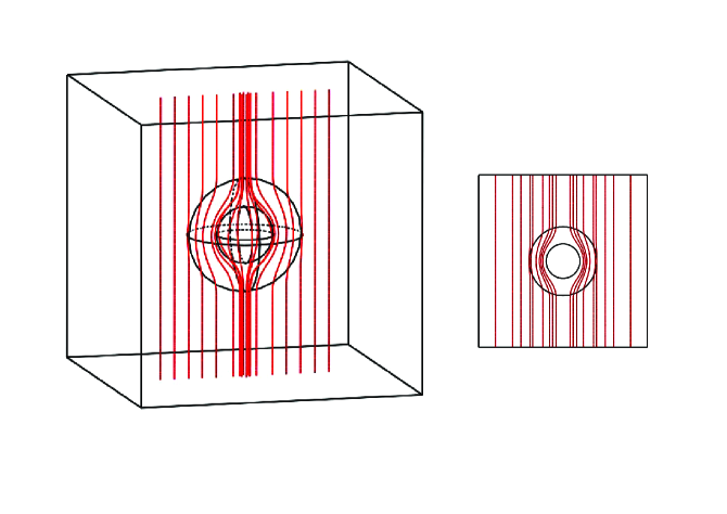
Figure 1:

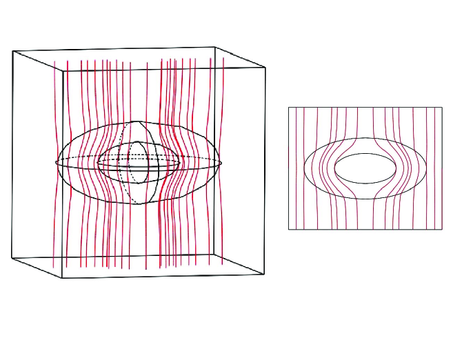
Figure 2:

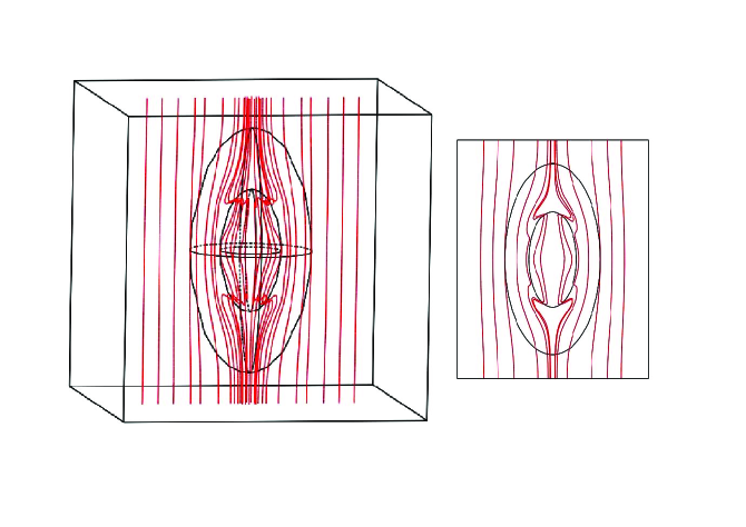
Figure 3:

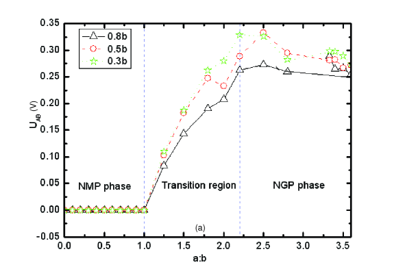
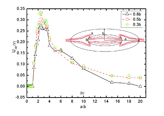
Figure 4:

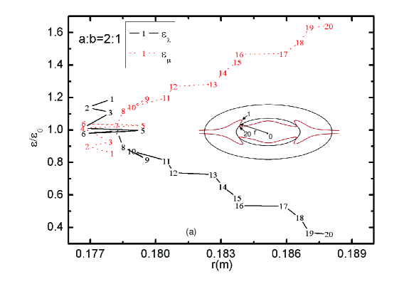
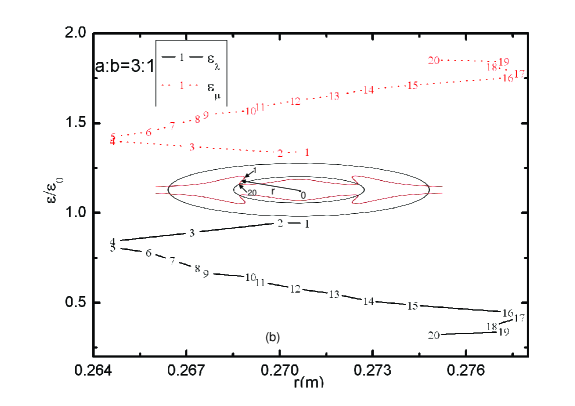
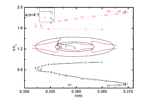
Figure 5:

Table 1: Cloaking efficiency of spherical and prolate spheroidal ($a>b=c$) cloaks. The external DC electric field is applied along the $a$, $b$, and $c$ principal semi-axes, respectively. $r_{1}$ (or $r_{2}$) denotes the inner (or outer) radius of a spherical cloak.

	shape        direction	inner	outer	$\eta$
	sphere	$r_{1}=0.1\,$m	$r_{2}=0.2\,$m	99.58%
	spheroid        $a$	$a_{1}=0.2\,$m, $b_{1}=0.1\,$m, $c_{1}=0.1\,$m	$a_{2}=0.4\,$m, $b_{2}=0.2\,$m, $c_{2}=0.2\,$m	99.14%
	spheroid        $b$ or $c$	$a_{1}=0.2\,$m, $b_{1}=0.1\,$m, $c_{1}=0.1\,$m	$a_{2}=0.4\,$m, $b_{2}=0.2\,$m, $c_{2}=0.2\,$m	99.15%

Table 2: Cloaking efficiency of oblate spheroidal ($a<b=c$) cloaks.

	shape        direction	inner	outer	$\eta$
	spheroid        $a$	$a_{1}=0.1\,$m, $b_{1}=0.2\,$m, $c_{1}=0.2\,$m	$a_{2}=0.2\,$m, $b_{2}=0.4\,$m, $c_{2}=0.4\,$m	97.75%
	spheroid        $b$ or $c$	$a_{1}=0.1\,$m, $b_{1}=0.2\,$m, $c_{1}=0.2\,$m	$a_{2}=0.2\,$m, $b_{2}=0.4\,$m, $c_{2}=0.4\,$m	97.69%

Table 3: Cloaking efficiency of ellipsoidal ($a\neq b\neq c$) cloaks.

	shape        direction	inner	outer	$\eta$
	ellipsoid        $a$	$a_{1}=0.1\,$m, $b_{1}=0.2\,$m, $c_{1}=0.4\,$m	$a_{2}=0.2\,$m, $b_{2}=0.4\,$m, $c_{2}=0.8\,$m	99.55%
	ellipsoid        $b$	$a_{1}=0.1\,$m, $b_{1}=0.2\,$m, $c_{1}=0.4\,$m	$a_{2}=0.2\,$m, $b_{2}=0.4\,$m, $c_{2}=0.8\,$m	99.56%
	ellipsoid        $c$	$a_{1}=0.1\,$m, $b_{1}=0.2\,$m, $c_{1}=0.4\,$m	$a_{2}=0.2\,$m, $b_{2}=0.4\,$m, $c_{2}=0.8\,$m	99.52%

References

- (1) V. G. Veselago, Soviet Physics USPEKI 10, 509 (1968)
- (2) J. B. Pendry, A. J. Holden, W. J. Stewart, and I. Youngs, Phys. Rev. Lett. 76, 4773 (1996)
- (3) J. B. Pendry, D. Schurig, and D. R. Smith, Science 312, 1780 (2006)
- (4) D. Schurig, J. B. Pendry and D. R. Smith, Opt. Express 14, 9794 (2006)
- (5) D. Schurig, J. J. Mock, B. J. Justice, S. A. Cummer, J. B. Pendry, A. F. Starr, and D. R. Smith, Science 314, 977 (2006)
- (6) D. R. Smith, J. B. Pendry, and M. C. K. Wiltshire, Science 305, 788 (2004)
- (7) Z. Ruan, M. Yan, C. W. Neff, and M. Qiu, Phys. Rev. Lett. 99, 113903 (2007)
- (8) M. Yan, Z. Ruan, and M. Qiu, Phys. Rev. Lett. 99, 233901 (2007)
- (9) H. Chen, B. Wu, B. Zhang, and J. A. Kong, Phys. Rev. Lett. 99, 063903 (2007)
- (10) W. Cai, U. K. Chettiar, A. V. Kildishev, and V. M. Shalaev, Nature Photonics 1, 224 (2007)
- (11) H. Y. Chen and C. T. Chan, Appl. Phys. Lett. 91, 183518 (2007)