Switching phenomena in magnetic vortex dynamics

Abstract

A magnetic nanoparticle in a vortex state is a promising candidate for the information storage. One bit of information corresponds to the upward or downward magnetization of the vortex core (vortex polarity). Generic properties of the vortex polarity switching are insensitive of the way how the vortex dynamics was excited: by an AC magnetic field, or by an electrical current. We study theoretically the switching process and describe in detail its mechanism, which involves the creation and annihilation of an intermediate vortex-antivortex pair.

Introduction

Artificial mesoscopic magnetic structures provide now a wide testing area for concepts of nanomagnetism and numerous prospective applications Hubert and Schäfer (1998); Skomski (2003). Investigations of magnetic nanostructures include studies of magnetic nanodots, which are submicron disk-shaped particles, which have a single vortex in the ground state due to the competition between exchange and magnetic dipole-dipole interaction Hubert and Schäfer (1998). A vortex state is obtained in nanodots that are larger than a single domain whose size is a few nanometers: e.g. for the Permalloy (Ni₈₀Fe₂₀) nanodot the exchange length $\ell\approx 5$ nm. Having nontrivial topological structure on the scale of a nanomagnet, the magnetic vortex is a promising candidate for the high density magnetic storage and high speed magnetic random access memory Cowburn (2002). For this one needs to control magnetization reversal, a process in which vortices play a big role Guslienko et al. (2001). Great progress has been made recently with the possibility to observe high frequency dynamical properties of the vortex state in magnetic dots by Brillouin light scattering of spin waves Demokritov et al. (2001); Hillebrands and Ounadjela (2002), time-resolved Kerr microscopy Park et al. (2003), phase sensitive Fourier transformation technique Buess et al. (2004), X-ray imaging technique Choe et al. (2004), and micro-SQUID technique Thirion et al. (2003).

The control of magnetic nonlinear structures using an electrical current is of special interest for applications in spintronics Tserkovnyak et al. (2005); Bader (2006). The spin torque effect, which is the change of magnetization due to the interaction with an electrical current, was predicted by Slonczewski (1996) and Berger (1996) in 1996. During the last decade this effect was tested in different magnetic systems Tsoi et al. (1998); Myers et al. (1999); Krivorotov et al. (2005) and nowadays it plays an important role in spintronics Tserkovnyak et al. (2005); Marrows (2005). Recently the spin torque effect was observed in vortex state nanoparticles. In particular, circular vortex motion can be excited by an AC Kasai et al. (2006) or a DC Pribiag et al. (2007) spin-polarized current. Very recently it was predicted theoretically Caputo et al. (2007a); Sheka et al. (2007) and observed experimentally Yamada et al. (2007) that the vortex polarity can be controlled using a spin-polarized current. This opens up the possibility of realizing electrically controlled magnetic devices, changing the direction of modern spintronics Cowburn (2007).

The basics of the magnetic vortex Kov statics and dynamics in Heisenberg magnets was studied in 1980s, in particular by the group of Kosevich Kosevich et al. (1983, 1985, 1990). Typically, the vortex is considered as a rigid particle without internal degrees of freedom; such a vortex undergoes a so-called gyroscopic dynamics in the framework of Thiele-like equations Thiele (1973); Huber (1982); Nikiforov and Sonin (1983). Using a rigid vortex dynamics a number of dynamical effects were studied, for a review see Ref. Mertens and Bishop (2000). Cycloidal oscillations around the mean vortex trajectory can be explained by taking into account changes of the vortex shape due to its velocity Mertens and Bishop (2000); Kovalev et al. (2003).

The rigid approach also fails when considering the vortex dynamics under the influence of a strong or fast external force. In particular, it is known that external pumping excites internal modes in vortex dynamics in Heisenberg magnets, whose role is important for understanding the switching phenomena Gaididei et al. (1999, 2000); Kovalev and Prilepsky (2002, 2003); Zagorodny et al. (2003), and the limit cycles in vortex dynamics Zagorodny et al. (2004); Sheka et al. (2005).

Very recently we have found that under the action of a magnetic field, or, alternatively, under the action of a spin current on a vortex state nanodot, the vortex core magnetization (polarity) can be switched. This effect was studied in Ref. Caputo et al. (2007a) analytically and confirmed numerically by direct spin-lattice simulations for Heisenberg magnets. However, the presence of the long-range dipolar interaction crucially changes the vortex dynamics Sheka et al. (2007), because this interaction creates an effective nonhomogeneous anisotropy Caputo et al. (2007a). The goal of this paper is to consider the generic properties of polarity switching in magnetic nanodots.

I Model and equations of motion

The magnetic energy of nanodots consists of two parts: Heisenberg exchange and dipolar interactions

$$\begin{split}\mathcal{H}&=-\frac{\ell^{2}}{2}\!\!\sum_{\left(\bm{n},\bm{\delta}\right)}\!\bm{S}_{\bm{n}}\cdot\bm{S}_{\bm{n}+\bm{\delta}}\\ &+\frac{1}{8\pi}\!\!\sum_{\begin{subarray}{c}\bm{n},\bm{n}^{\prime}\\ \bm{n}\neq\bm{n}^{\prime}\end{subarray}}\!\frac{\bm{S}_{\bm{n}}\cdot\bm{S}_{\bm{n}^{\prime}}-3\left(\bm{S}_{\bm{n}}\cdot\bm{e}_{\bm{n}\bm{n}^{\prime}}\right)\left(\bm{S}_{\bm{n}^{\prime}}\cdot\bm{e}_{\bm{n}\bm{n}^{\prime}}\right)}{|\bm{n}-\bm{n}^{\prime}|^{3}}\end{split}$$ (1)

Here $\bm{S}_{\bm{n}}$ is a unit vector which determines the spin direction at the lattice point $\bm{n}$, $\ell=\sqrt{A/(\mu_{0}M_{S}^{2})}$ is the exchange length ($A$ is the exchange constant, $\mu_{0}$ is the vacuum permeability, $M_{S}$ is the saturation magnetization), the vector $\bm{\delta}$ connects nearest neighbors, and $\bm{e}_{\bm{n}\bm{n}^{\prime}}\equiv(\bm{n}-\bm{n}^{\prime})/|\bm{n}-\bm{n}^{\prime}|$ is a unit vector. The lattice constant is chosen as a unity length.

It is known that as a result of the competition between the exchange and the dipolar interactions the ground state of a thin magnetically soft nanodisk is a vortex state: the magnetization lies in the XY disk plane in the main part of the disk and is parallel to the disk edge, forming the magnetic flux-closure pattern characterized by the vorticity $q=+1$. At the disk center the magnetization distribution forms a vortex core, which is oriented either parallel or antiparallel to the z-axis. The former is characterized by a polarity $p=+1$ and the latter by $p=-1$.

The spin dynamics of the system is described by the modified Landau–Lifshitz–Gilbert equation

$$\dot{\bm{S}_{\bm{n}}}=-\bm{S}_{\bm{n}}\times\frac{\partial\mathcal{H}}{\partial\bm{S}_{\bm{n}}}-\alpha\bm{S}_{\bm{n}}\times\dot{\bm{S}_{\bm{n}}}+\bm{S}_{\bm{n}}\times\bm{b}_{\bm{n}}.$$ (2)

Here the overdot indicates the derivative with respect to the dimensionless time $\tau=\omega_{0}t$ with $\omega_{0}=4\pi\gamma M_{S}$, $\alpha\ll 1$ is a damping coefficient. The last term is a spin torque due to external forces, which results in a magnetic field $\bm{b}_{\bm{n}}$. In the presence of the homogeneous rotating field $\bm{B}(t)=\left(B\cos\omega\tau,B\sin\omega\tau,0\right)$, the dimensionless field

$$\bm{b}=b_{x}+{i}b_{y}=\frac{B}{4\pi M_{S}}\exp({i}\omega\tau).$$ (3a)

Here and below all frequencies are measured in units of $$\omega_{0} \ell$$, and all distances in units of .

When an electrical current is injected in the pillar structure, perpendicular to the nanodisk plane, it influences locally the spin $\bm{S}_{\bm{n}}$ of the lattice through the spin torque $\bm{T}_{\bm{n}}=\bm{S}_{\bm{n}}\times\bm{b}_{\bm{n}}$ Slonczewski (1996); Berger (1996), where

$$\bm{b}_{\bm{n}}=j\,\sigma\mathcal{A}\frac{\bm{S}_{\bm{n}}\times\hat{\bm{z}}}{1+\sigma\mathcal{B}\bm{S}_{n}\cdot\hat{\bm{z}}}.$$ (3b)

Here $j=J_{e}/J_{p}$ is a normalized spin current, $J_{e}$ is the electrical current density, $J_{p}=\mu_{0}M_{S}^{2}|e|h/\hslash$, $h$ is the disk thickness, $e$ is the electron charge, $\mathcal{A}=4\eta_{sp}^{3/2}/\left[3(1+\eta_{sp})^{3}-16\eta_{sp}^{3/2}\right]$, $\mathcal{B}=(1+\eta_{sp})^{3}/\left[3(1+\eta_{sp})^{3}-16\eta_{sp}^{3/2}\right]$, and $\eta_{sp}\in(0;1)$ denotes the degree of the spin polarization; $\sigma=\pm 1$ gives two directions of the spin-current polarization.

II Vortex structure and Rigid vortex dynamics

In the case of weak dipolar interactions, the characteristic exchange length $\ell$ is larger than the lattice constant $a$, so that in the lowest approximation in the small parameter $a/\ell$ and weak gradients of magnetization $\bm{m}=-\langle\bm{S}_{\bm{n}}\rangle=\left(\sin\theta\cos\phi,\sin\theta\sin\phi,\cos\theta\right)$ we can use the continuum approximation for the Hamiltonian (1).

$$\mathscr{E}=\int\mathrm{d}^{2}x\left[\frac{\ell^{2}}{2}\left(\bm{\nabla}{\bm{m}}\right)^{2}-\frac{\bm{m}\cdot\bm{H}^{\text{ms}}}{2}-\bm{m}\cdot\bm{b}\right],$$ (4)

where $\bm{H}^{\text{ms}}$ is the normalized magnetostatic field, which comes from the dipolar interaction Akhiezer et al. (1968). In (4) we suppose that the magnetization distribution does not depend on the $z$-component (which is valid for thin disks) and we have normalized the energy by the disk thickness $h$.

Let us consider a cylindric nanoparticle of top surface radius $L$ and thickness $h$. For small size nanoparticles the ground state is uniform; it depends on the particle aspect ratio $\varepsilon=h/(2L)$: thin nanodisks are magnetized in the plane (when $\varepsilon<\varepsilon_{c}\approx 0.906$ Aharoni (1990)) and thick ones along the axis (when $\varepsilon>\varepsilon_{c}$). When the particle size exceeds some critical value, typically $(3-4)\ell$ Ross et al. (2002), the magnetization curling becomes energetically preferable due to the competition between the exchange and dipolar interactions. For a disk-shaped particle there appears the vortex state. For thin enough disks the vortex structure does not depend on the $z$-coordinate of the disk and the magnetization distribution for the vortex, which is situated in the disk center, is determined by the expressions Mertens and Bishop (2000)

$$\cos\theta=pf(|\zeta|),\qquad\phi=q\arg\zeta+C\pi/2.$$ (5a)

Here $$\zeta=x+{i}y q=+1 \pi_{1} C=\pm 1 p=\pm 1 f(|\zeta|) \pi_{2}$$ is the coordinate in the disk plane, is the vortex topological charge (vorticity), characterizes the vortex chirality, and determines the direction of the vortex core magnetization (polarity). The bell-shaped function describes the vortex core magnetization. The vortex polarity is connected to the topological properties of the system, the Pontryagin index

$$Q=\frac{1}{8\pi}\int\mathrm{d}^{2}x\epsilon_{ij}\bm{m}\cdot\left[\partial_{j}\bm{m}\times\partial_{j}\bm{m}\right].$$

For the vortex configuration the Pontryagin index takes the half-integer values $$Q=-pq/2$$.

For the vortex solution localized at $Z=X+{i}Y=R\exp({i}\Phi)$, the $\phi$-field has the form $\phi=q\arg(\zeta-Z)+C\pi/2.$ Such a form of the $\phi$–field satisfies the Laplace equation, so it describes the planar vortex dynamics (neglecting the z-component of magnetization) for the infinite Heisenberg magnets. The finite size effects for the circular Heisenberg magnet can be described by the image-vortex ansatz Mertens and Bishop (2000). Moreover, one has to take into account the long-range dipolar interactions, which lead in general to integro-differential equations Guslienko and Novosad (2004). For a thin ferromagnet the dipolar interactions produce an effective uniaxial anisotropy of the easy-plane type caused by the faces surface magnetostatic charges Gioia and James (1997); Ivanov and Zaspel (2002) and an effective in-plane anisotropy caused by the edge surface charges (surface anisotropy) Carbou (2001); Ivanov and Zaspel (2002). Due to the surface anisotropy the magnetization near the disk edge is constrained to be tangential to the boundary, which prevents its precession near the edge (absence of surface charges) Ivanov and Zaspel (2002); Guslienko and Slavin (2005); Caputo et al. (2007b). Finally, the $\phi$–field can be written in the form

$$\phi=\arg\bigl{[}\zeta-Z\bigr{]}+\arg\bigl{[}\zeta-Z^{I}\bigr{]}-\arg Z+C\frac{\pi}{2}.$$ (5b)

Here $Z^{I}=ZL^{2}/R^{2}$ is the image vortex coordinate; the image vortex is added to satisfy the Dirichlet boundary conditions.

Under the influence of an external force the vortex starts to move. If such forces are weak, the vortex behaves like a particle during its evolution. Such rigid vortex dynamics can be well-described using the Thiele approach Thiele (1973); Huber (1982). Following this approach we use the traveling wave ansatz $\bm{m}(\bm{r},\tau)=\bm{m}(\bm{r}-\bm{R}(\tau))$, where the function $\bm{m}$ on the right–hand side describes the vortex shape (5). This results in a force balance equation $\bm{F}^{g}+\bm{F}^{d}+\bm{F}=0$. The first term $\bm{F}^{g}=-2Q\left[\dot{\bm{R}}\times\hat{\bm{z}}\right]$ is a gyroscopical force Huber (1982); Nikiforov and Sonin (1983), which acts on a moving vortex in the same way as the magnetic field influences a charged particle by a Lorentz force. The second term is a dissipative force $\bm{F}^{d}=-\eta\dot{\bm{R}}$ with $\eta\approx(\alpha/2)\ln L$, and the last term is an external force $\bm{F}=-(2\pi)^{-1}\bm{\nabla}_{\bm{R}}\mathscr{E}=\bm{F}^{\text{ms}}+\bm{F}^{\text{ext}}$, where the total energy is described by Eq. (4). The magnetostatic part of this force is caused mainly by magnetostatic energy of volume charges. For small displacements $R\ll L$ from the disk origin and small aspect ratios ($\varepsilon\ll 1$), it can be found analytically that $\bm{F}^{\text{ms}}=-\Omega_{G}\bm{R}$ Guslienko et al. (2002) with $\Omega_{G}\sim 10\varepsilon/9\pi$ Guslienko et al. (2006). For finite $\varepsilon$ one can use the analysis in Ref. Ivanov and Zaspel (2004); Zaspel et al. (2005), which results in $\Omega_{G}(\varepsilon)$. Finally the force balance condition takes the form of a Thiele equation

$$2Q\left[\dot{\bm{R}}\times\hat{\bm{z}}\right]=\bm{F}^{\text{ext}}-\eta\dot{\bm{R}}-\Omega_{G}\bm{R}.$$ (6)

Without dissipation and external force this equation describes a gyration of the vortex around the disk origin with a frequency $\Omega_{G}$. The dissipation damps the possible circular motion of the vortex. However, an external force can excite a non-decaying vortex motion. For example, it is known that the rotating magnetic field can excite a circular rotation of the vortex in a Heisenberg magnet Zagorodny et al. (2004); Sheka et al. (2005) and a nanomagnet Kravchuk et al. (2007) due to the force Sheka et al. (2005)

$$\bm{F}^{\text{ext}}\!=\!-\frac{bL}{2R}\Bigl{\{}\!\bm{R}\cos(\Phi-\omega\tau)+\left[\bm{R}\times\hat{\bm{z}}\right]\sin(\Phi-\omega\tau)\!\Bigr{\}}.$$ (7a)

In the case of electrical current influence the circular vortex dynamics can be excited by the force Liu et al. (2007a); Ivanov and Zaspel (2007); Sheka et al. (2008):

$$\bm{F}^{\text{ext}}=\frac{j\sigma\mathcal{A}q}{2\omega_{0}}\left[\bm{R}\times\hat{\bm{z}}\right].$$ (7b)

Note that the vortex motion can be excited by any small magnetic field $(b,\omega)$ Kravchuk et al. (2007); howeber, to excite the vortex motion by a spin current, its intensity should exceed threshold value Ivanov and Zaspel (2007); Sheka et al. (2008).

III Numerical studies

In order to check the analytical predictions about the driven vortex dynamics, we have performed numerical simulations. In the case of a rotating magnetic field we used the micromagnetic simulator for Landau-Lifshitz-Gilbert equations OOM as described in Ref. Kravchuk et al. (2007). To study the vortex dynamics under the action of a spin-polarized electrical current, we used numerical simulations of the discrete spin-lattice Eq. (2) with the spin torque given by Eq. (3b) as described in Refs. Sheka et al. (2007, 2008). In both cases, as initial condition we use the vortex with positive polarity ($p=+1$), centered at the disk origin. To identify precisely the vortex position we use, similar to Ref. Hertel and Schneider (2006), the crossection of isosurfaces $m_{x}=0$ and $m_{y}=0$.

Let us start with the case of a spin current. If we apply the current, whose polarization is parallel to the vortex polarity ($j\sigma p>0$), the vortex does not quit the disk center, which is a stable point. However, if the spin current has the opposite direction of the spin polarization ($j\sigma p<0$, $p=+1$, $\sigma=+1$ and $j<0$ in our case) the vortex motion can be excited when the current intensity is above a threshold value Liu et al. (2007a); Ivanov and Zaspel (2007); Sheka et al. (2008) as a result of the balance between the pumping and damping. Following the spiral trajectory, the vortex finally reaches a circular limit cycle. The rotation sense of the spiral is determined by the gyroforce, i.e. by the topological charge $Q$, which is a clockwise rotation in our case. At some value, the radius becomes comparable with the system size $L$ and the vortex dynamics becomes more complicated and can not be described by the Thiele equation (6). Finally it results in a switching of the vortex core, see below.

A qualitatively similar picture is found in the case of a rotating field with angular frequency directed opposite to the vortex polarity: $\omega p<0$. There exist different regimes in the vortex dynamics Kravchuk et al. (2007). In the range of frequencies close to the frequency of the orbital vortex motion ($\Omega\sim 1$ GHz) the vortex demonstrates a finite motion in a region near the disk center along a quite complicated trajectory and does not switch its polarity. These cycloidal vortex oscillations are similar to those in Ref. Kovalev et al. (2003), and correspond to the excitation of higher magnon modes during the motion. If $\omega\gg\Omega$, then for weak fields the vortex motion can be considered as a sum of two constituents: (i) the gyroscopic orbital motion as without field, and (ii) cycloidal oscillations caused by the field influence. For the case $\omega p<0$ the direction of the cycloidal oscillations coincides with the direction of the field rotation, while the direction of the gyroscopic orbital motion is opposite to it. For stronger fields the vortex motion becomes more complicated and its average motion can be directed even opposite to the gyroscopical motion (this situation is shown in Fig. 1). The irreversible switching of the vortex polarity can be excited in a specific range of parameters $(\omega,b)$, with typical frequencies about $10$ GHz and intensities about $20$ mT Kravchuk et al. (2007). The mechanism of the switching is discussed below.

IV Vortex polarity switching

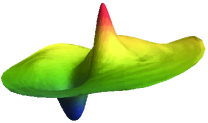
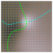
(a) t=110 ps: the rotating field causes the vortex motion, as a result a negative dip is forming.

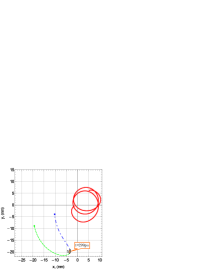
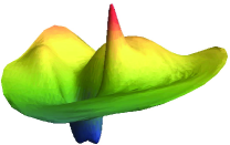
(b) t=320 ps: a vortex-antivortex pair has been born in region 1.

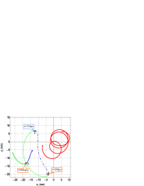
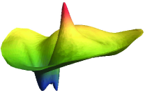
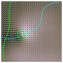
(c) t=420 ps: the vortex pair has annihilated in region 2, after some time a new vortex-antivortex pair is born in region 3.

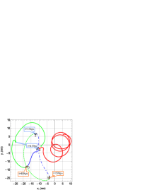
(d) t=495 ps: the new antivortex has annihilated with the old vortex in region 4 and only the new vortex of opposite polarity remains.

Figure 1: The vortex switching process under rotating field influence. Left column – vortex trajectories. Red line – initial vortex core trajectory, green line – new vortex, blue line – antivortex. Right column – in-plane magnetization distribution, the out-of-plane component is denoted by levels of gray color, dashed blue and solid green lines correspond to isosurfaces $m_{x}=0$ and $m_{y}=0$, respectively. The out-of-plane component $m_{z}$ is shown in the middle column. The data were obtained from micromagnetic simulation for a permalloy disk (132nm diam., 20nm thickness) dynamics under rotating field ($B=0.07$ T, $\omega=10$ GHz) influence.

The mechanism of the vortex switching is of general nature; it is essentially the same in all systems where the switching was observed Waeyenberge et al. (2006); Xiao et al. (2006); Hertel et al. (2007); Lee et al. (2007); Yamada et al. (2007); Kravchuk et al. (2007); Sheka et al. (2007); Liu et al. (2007a). Under the action of pumping, the original vortex (V, $q_{V}=1,p_{V}=1,Q_{V}=-1/2$), situated in the disk center, moves along a spiral trajectory in the case of a current or along a more complicated trajectory (as described in the previous section) in the case of the rotating field. During its motion, the vortex excites a number of spin waves Choi et al. (2007). Mainly magnon modes of two kinds are excited in this system: symmetrical and azimuthal ones Gaididei et al. (2000); Zagorodny et al. (2003). Due to the continuous pumping the system goes to the nonlinear regime: the amplitude of the azimuthal mode increases and there appears an out-of-plane dip nearby the vortex, see Fig. 1(a). When the amplitude of the out-of-plane dip reaches its minimum [$m_{z}=-1$, Fig. 1(b)] a pair of a new vortex (NV, $q_{NV}=-1,p_{NV}=-1,Q_{NV}=-1/2$) and antivortex (AV, $q_{AV}=1,p_{AV}=-1,Q_{AV}=1/2$) is created. These three objects move following complicated trajectories which result from Thiele-like equations. The directions of the motion of the partners are determined by the competition between the gyroscopical motion and the external forces, which are magnetostatic force $F^{\text{ms}}$, pumping force $F^{\text{ext}}$, see Eqs. (7), and the interactions between the vortices $\bm{F}_{i}^{\text{int}}$.

The magnetostatic force for the three body system can be calculated, using the image vortex approach, which corresponds to fixed (Dirichlet) boundary conditions. For the vortex state nanodisk such boundary conditions results from the magnetostatic interaction, which is localized near the disk edge Ivanov and Zaspel (2002). The same statement is also valid for the three vortex (V-AV-NV) state, which is confirmed also by our numerical simulations. The $\phi$–field can be presented by the three vortex ansatz

$$\phi=\sum_{i=1}^{3}q_{i}\Bigl{\{}\arg\bigl{[}\zeta-Z_{i}\bigr{]}+\arg\bigl{[}\zeta-Z_{i}^{I}\bigr{]}-\arg Z_{i}\Bigr{\}}+C\frac{\pi}{2}.$$ (8)

The force coming from the volume magnetostatic charge density $\lambda=-\bm{\nabla}\cdot\bm{m}$ can be calculated in the same way as for a single vortex Metlov and Guslienko (2002); Ivanov and Zaspel (2007), which results in $\bm{F}^{\text{ms}}\approx-\Omega_{G}q_{i}\sum_{j}q_{j}\bm{R_{j}}$, where $q_{i}=\pm 1$ is the vorticity of $i$-th vortex (antivortex).

The interaction force $\bm{F}^{\text{int}}$ between vortices is a 2D coulomb force $\bm{F}_{i}^{\text{int}}=\sum\limits_{i\neq j}q_{i}q_{j}\frac{\bm{R}_{i}-\bm{R}_{j}}{\left|\bm{R}_{i}-\bm{R}_{j}\right|^{2}}$.

The internal gyroforces of the dip impart the initial velocities to the NV and AV, which are perpendicular to the initial dip velocity and have opposite directions. In this way the AV gains the velocity component directed to the center, where the V is moving. This new-born pair is a topologically trivial $Q=0$ pair, which undergoes a Kelvin motion Papanicolaou and Spathis (1999). This Kelvin pair collides with the original vortex. If the pair was born far from V then the scattering process is semi–elastic; the new-born pair is not destroyed by the collision. In the exchange approach this pair survives, but it is scattered by some angle Komineas and Papanicolaou (2007). Due to additional forces (pumping, damping and magnetostatic interaction), the real motion is more complicated and the Kevin pair can finally annihilate by itself, see Fig. 1(c).

Another collision mechanism takes place when the pair is born closer to the original vortex. Then the AV can be captured by the V and an annihilation with the original vortex happens, see Fig. 1(d). The collision process is essentially inelastic. During the collision, the original vortex and the antivortex form a topological nontrivial pair ($Q=-1$), which performs a rotational motion around some guiding center Komineas (2007); Komineas and Papanicolaou (2007). This rotating vortex dipole forms a localized skyrmion (Belavin-Polyakov soliton Belavin and Polyakov (1975)), which is stable in the continuum system. In the discrete lattice system the radius of this soliton, i.e. the distance between vortex and antivortex, rapidly decreases almost without energy loss. When the soliton radius is about one lattice constant, the pair undergoes the topologically forbidden annihilation Kravchuk et al. (2007); Komineas (2007), which is accompanied by strong spin-wave radiation, because the topological properties of the system change Hertel and Schneider (2006); Tretiakov and Tchernyshyov (2007).

The three–body problem can be analytically described in a rigid vortex approach, based on Thiele-like equations (6):

$$\begin{split}&2Q_{i}\left[\dot{\bm{R}}_{i}\times\hat{\bm{z}}\right]=\sum_{i\neq j}q_{i}q_{j}\frac{\bm{R}_{i}-\bm{R}_{j}}{\left\lvert\bm{R}_{i}-\bm{R}_{j}\right\rvert^{2}}+\bm{F}_{i}^{\text{ext}}\\ &-\eta\dot{\bm{R}}_{i}-\Omega_{G}(\varepsilon)q_{i}\sum\limits_{j}q_{j}\bm{R}_{j},\qquad i=1,2,3.\end{split}$$ (9)

Here $\bm{F}_{i}^{\text{ext}}$ is the driving force (7), caused by the field (7a) or spin-current (7b) pumping. This three–body process in exchange interaction approximation is studied in detail by Komineas and Papanicolaou (2007).

The set of Eqs. (9) describes the main features of the observed three–body dynamics. During the evolution, the original vortex and the antivortex create a rotating dipole, in agreement with Refs. Komineas (2007); Komineas and Papanicolaou (2007), see Fig. 2. The distance in this vortex dipole rapidly tends to zero. The new–born vortex moves on a clockwise spiral to the origin.

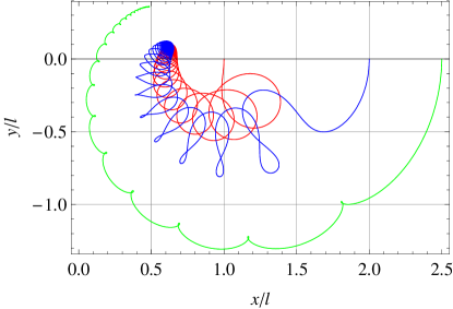
Figure 2: Three–body dynamics from the solution of Eq. (9), for a system with $L/\ell=20$, $\alpha=0.01$, $b=0.02$, $\omega=1$, and $\Omega_{G}=0.0287$. The original vortex (red line) was positioned at $(1,0)\ell$, the antivortex (blue) at $(2,0)\ell$, and the newborn vortex (green) at $(2.5,0)\ell$.

V Summary

To summarize, we have studied the switching of the magnetic vortex polarity under the action of a rotating magnetic field and under the action of a spin-polarized current. The switching picture involving the creation and annihilation of a vortex-antivortex pair is very general and does not depend on the details how the vortex dynamics was excited. In particular, such a switching mechanism can be induced by a field pulse Waeyenberge et al. (2006); Xiao et al. (2006); Hertel et al. (2007), by an AC oscillating Lee et al. (2007) or rotating field Kravchuk et al. (2007), by an in-plane electrical current (nonhomogeneous spin torque) Yamada et al. (2007); Liu et al. (2007b) and by a perpendicular current (homogeneous spin torque) Sheka et al. (2007); Liu et al. (2007a); Ivanov and Zaspel (2007). Our analytical analysis is confirmed by numerical spin-lattice simulations.

The authors acknowledge support from Deutsches Zentrum für Luft- und Raumfart e.V., Internationales Büro des Bundesministeriums für Forschung und Technologie, Bonn, in the frame of a bilateral scientific cooperation between Ukraine and Germany, project No. UKR 05/055. Yu.G., V.P.K. and D.D.S. thank the University of Bayreuth, where a part of this work was performed, for kind hospitality. Yu. G. acknowledges support from the Special Program of Department of Physics and Astronomy of the National Academy of Sciences of Ukraine. V.P.K. and D.D.S. acknowledge support from the grant No. F25.2/081 from the Fundamental Researches State Fund of Ukraine. D.D.S. acknowledges also the support from the Alexander von Humboldt–Foundation.

References

- Hubert and Schäfer (1998) A. Hubert and R. Schäfer, Magnetic domains (Springer–Verlag, Berlin, 1998).
- Skomski (2003) R. Skomski, J. Phys. C 15, R841 (2003), URL http://dx.doi.org/10.1088/0953-8984/15/20/202.
- Cowburn (2002) R. P. Cowburn, J. Magn. Magn. Mater. 242-245, 505 (2002), URL http://dx.doi.org/10.1016/S0304-8853(01)01086-1.
- Guslienko et al. (2001) K. Y. Guslienko, V. Novosad, Y. Otani, H. Shima, and K. Fukamichi, Phys. Rev. B 65, 024414 (2001), URL http://dx.doi.org/10.1103/PhysRevB.65.024414.
- Demokritov et al. (2001) S. O. Demokritov, B. Hillebrands, and A. N. Slavin, Physics Reports 348, 441 (2001), URL http://www.sciencedirect.com/science/article/B6TVP-43B29GN-1/%2/92cce5adca2ce19b207e73d018666fcf.
- Hillebrands and Ounadjela (2002) B. Hillebrands and K. Ounadjela, eds., Spin dynamics in confined magnetic structures I, vol. 83 of Topics in Applied Physics (Springer, Berlin, 2002).
- Park et al. (2003) J. P. Park, P. Eames, D. M. Engebretson, J. Berezovsky, and P. A. Crowell, Phys. Rev. B 67, 020403 (2003), URL http://link.aps.org/abstract/PRB/v67/e020403.
- Buess et al. (2004) M. Buess, R. Hŏllinger, T. Haug, K. Perzlmaier, U. K. D. Pescia, M. R. Scheinfein, D.Weiss, and C. H. Back, Phys. Rev. Lett. 93, 077207 (2004), URL http://dx.doi.org/10.1103/PhysRevLett.93.077207.
- Choe et al. (2004) S.-B. Choe, Y. Acremann, A. Scholl, A. Bauer, A. Doran, J. Stohr, and H. A. Padmore, Science 304, 420 (2004), eprint http://www.sciencemag.org/cgi/reprint/304/5669/420.pdf, URL http://www.sciencemag.org/cgi/content/abstract/304/5669/420.
- Thirion et al. (2003) C. Thirion, W. Wernsdofer, and D. Mailly, Nature Materials 2, 524 (2003).
- Tserkovnyak et al. (2005) Y. Tserkovnyak, A. Brataas, G. E. W. Bauer, and B. I. Halperin, Rev. Mod. Phys. 77, 1375 (pages 47) (2005), URL http://link.aps.org/abstract/RMP/v77/p1375.
- Bader (2006) S. D. Bader, Rev. Mod. Phys. 78, 1 (pages 15) (2006), URL http://link.aps.org/abstract/RMP/v78/p1.
- Slonczewski (1996) J. C. Slonczewski, J. Magn. Magn. Mater. 159, L1 (1996), URL http://dx.doi.org/10.1016/0304-8853(96)00062-5.
- Berger (1996) L. Berger, Phys. Rev. B 54, 9353 (1996), URL http://link.aps.org/abstract/PRB/v54/p9353.
- Tsoi et al. (1998) M. Tsoi, A. G. M. Jansen, J. Bass, W.-C. Chiang, M. Seck, V. Tsoi, and P. Wyder, Phys. Rev. Lett. 80, 4281 (1998), URL http://dx.doi.org/10.1103/PhysRevLett.80.4281.
- Myers et al. (1999) E. B. Myers, D. C. Ralph, J. A. Katine, R. N. Louie, and R. A. Buhrman, Science 285, 867 (1999), URL http://dx.doi.org/10.1126/science.285.5429.867.
- Krivorotov et al. (2005) I. N. Krivorotov, N. C. Emley, J. C. Sankey, S. I. Kiselev, D. C. Ralph, and R. A. Buhrman, Science 307, 228 (2005), URL http://dx.doi.org/10.1126/science.1105722.
- Marrows (2005) C. H. Marrows, Advances in Physics 54, 585 (2005), ISSN 0001-8732, URL http://www.informaworld.com/10.1080/00018730500442209.
- Kasai et al. (2006) S. Kasai, Y. Nakatani, K. Kobayashi, H. Kohno, and T. Ono, Phys. Rev. Lett. 97, 107204 (pages 4) (2006), URL http://link.aps.org/abstract/PRL/v97/e107204.
- Pribiag et al. (2007) V. S. Pribiag, I. N. Krivorotov, G. D. Fuchs, P. M. Braganca, O. Ozatay, J. C. Sankey, D. C. Ralph, and R. A. Buhrman, Nat Phys 3, 498 (2007), ISSN 1745-2473, URL http://dx.doi.org/10.1038/nphys619.
- Caputo et al. (2007a) J.-G. Caputo, Y. Gaididei, F. G. Mertens, and D. D. Sheka, Phys. Rev. Lett. 98, 056604 (pages 4) (2007a), URL http://link.aps.org/abstract/PRL/v98/e056604.
- Sheka et al. (2007) D. D. Sheka, Y. Gaididei, and F. G. Mertens, Appl. Phys. Lett. 91, 082509 (2007), URL http://link.aip.org/link/?APL/91/082509/1.
- Yamada et al. (2007) K. Yamada, S. Kasai, Y. Nakatani, K. Kobayashi, H. Kohno, A. Thiaville, and T. Ono, Nat Mater 6, 270 (2007), ISSN 1476-1122, URL http://dx.doi.org/10.1038/nmat1867.
- Cowburn (2007) R. P. Cowburn, Nat Mater 6, 255 (2007), ISSN 1476-1122, URL http://dx.doi.org/10.1038/nmat1877.
- (25) To the best of our knowledge the term magnetic vortex was introduced by the Kosevich group in Ref. Kovalev et al. (1979) for the object, which is now called magnetic skyrmion and is widely used for the localized solitons, e.g. in easy-axis magnets.
- Kovalev et al. (1979) A. Kovalev, A. Kosevich, and K. Maslov, JETP Lett. 30, 296 (1979), URL http://www.jetpletters.ac.ru/ps/1365/article_20632.shtml.
- Kosevich et al. (1983) A. M. Kosevich, V. P. Voronov, and I. V. Manzhos, Sov. Phys. JETP 57, 148 (1983).
- Kosevich et al. (1985) A. M. Kosevich, B. A. Ivanov, and A. S. Kovalev, Sov. Sci. Rev. Sec.A. 6, 161 (1985).
- Kosevich et al. (1990) A. M. Kosevich, B. A. Ivanov, and A. S. Kovalev, Physics Reports 194, 117 (1990), URL http://www.sciencedirect.com/science/article/B6TVP-46SXP0P-19%/2/d0a99bbbccf078602123db3e5d601202.
- Thiele (1973) A. A. Thiele, Phys. Rev. Lett. 30, 230 (1973), URL http://link.aps.org/abstract/PRL/v30/p230.
- Huber (1982) D. L. Huber, Phys. Rev. B 26, 3758 (1982), URL http://link.aps.org/abstract/PRB/v26/p3758.
- Nikiforov and Sonin (1983) A. V. Nikiforov and É. B. Sonin, Soviet Physics - JETP 58, 373 (1983), URL http://link.aip.org/link/?SPJ/58/373/1.
- Mertens and Bishop (2000) F. G. Mertens and A. R. Bishop, in Nonlinear Science at the Dawn of the 21th Century, edited by P. L. Christiansen, M. P. Soerensen, and A. C. Scott (Springer–Verlag, Berlin, 2000).
- Kovalev et al. (2003) A. S. Kovalev, F. G. Mertens, and H. J. Schnitzer, Eur. Phys. J. B 33, 133 (2003), URL http://dx.doi.org/10.1140/epjb/e2003-00150-3.
- Gaididei et al. (1999) Y. Gaididei, T. Kamppeter, F. G. Mertens, and A. Bishop, Phys. Rev. B 59, 7010 (1999), URL http://link.aps.org/abstract/PRB/v59/p7010.
- Gaididei et al. (2000) Y. Gaididei, T. Kamppeter, F. G. Mertens, and A. R. Bishop, Phys. Rev. B 61, 9449 (2000), URL http://link.aps.org/abstract/PRB/v61/p9449.
- Kovalev and Prilepsky (2002) A. S. Kovalev and J. E. Prilepsky, Low Temp. Phys. 28, 921 (2002), URL http://dx.doi.org/10.1063/1.1531396.
- Kovalev and Prilepsky (2003) A. S. Kovalev and J. E. Prilepsky, Low Temp. Phys. 29, 55 (2003), URL http://dx.doi.org/10.1063/1.1542378.
- Zagorodny et al. (2003) J. P. Zagorodny, Y. Gaididei, F. G. Mertens, and A. R. Bishop, Eur. Phys. J. B 31, 471 (2003), URL http://dx.doi.org/10.1140/epjb/e2003-00057-y.
- Zagorodny et al. (2004) J. P. Zagorodny, Y. Gaididei, D. D. Sheka, J.-G. Caputo, and F. G. Mertens, Phys. Rev. Lett. 93, 167201 (pages 4) (2004), URL http://link.aps.org/abstract/PRL/v93/e167201.
- Sheka et al. (2005) D. D. Sheka, J. P. Zagorodny, J. G. Caputo, Y. Gaididei, and F. G. Mertens, Phys. Rev. B 71, 134420 (pages 15) (2005), URL http://link.aps.org/abstract/PRB/v71/e134420.
- Akhiezer et al. (1968) A. I. Akhiezer, V. G. Bar’yakhtar, and S. V. Peletminskiĭ, Spin waves (North–Holland, Amsterdam, 1968).
- Aharoni (1990) A. Aharoni, J. Appl. Phys. 68, 2892 (1990), URL http://link.aip.org/link/?JAP/68/2892/1.
- Ross et al. (2002) C. A. Ross, M. Hwang, M. Shima, J. Y. Cheng, M. Farhoud, T. A. Savas, H. I. Smith, W. Schwarzacher, F. M. Ross, M. Redjdal, et al., Phys. Rev. B 65, 144417 (2002), URL http://link.aps.org/abstract/PRB/v65/e144417.
- Guslienko and Novosad (2004) K. Y. Guslienko and V. Novosad, J. Appl. Phys. 96, 4451 (2004), URL http://link.aip.org/link/?JAP/96/4451/1.
- Gioia and James (1997) G. Gioia and R. D. James, Proc. R. Soc. Lond. A 453, 213 (1997), URL http://www.journals.royalsoc.ac.uk/openurl.asp?genre=article&%id=doi:10.1098/rspa.1997.0013.
- Ivanov and Zaspel (2002) B. A. Ivanov and C. E. Zaspel, Appl. Phys. Lett. 81, 1261 (2002), URL http://dx.doi.org/10.1063/1.1499515.
- Carbou (2001) G. Carbou, Mathematical Models and Methods in Applied Sciences (M3AS) 11, 1529 (2001), URL http:/dx.doi.org/10.1142/S0218202501001458.
- Guslienko and Slavin (2005) K. Y. Guslienko and A. N. Slavin, Phys. Rev. B 72, 014463 (pages 5) (2005), URL http://link.aps.org/abstract/PRB/v72/e014463.
- Caputo et al. (2007b) J.-G. Caputo, Y. Gaididei, V. P. Kravchuk, F. G. Mertens, and D. D. Sheka, Phys. Rev. B 76, 174428 (pages 13) (2007b), URL http://link.aps.org/abstract/PRB/v76/e174428.
- Guslienko et al. (2002) K. Y. Guslienko, B. A. Ivanov, V. Novosad, Y. Otani, H. Shima, and K. Fukamichi, J. Appl. Phys. 91, 8037 (2002), URL http://link.aip.org/link/?JAP/91/8037/1.
- Guslienko et al. (2006) K. Y. Guslienko, X. F. Han, D. J. Keavney, R. Divan, and S. D. Bader, Phys. Rev. Lett. 96, 067205 (pages 4) (2006), URL http://link.aps.org/abstract/PRL/v96/e067205.
- Ivanov and Zaspel (2004) B. A. Ivanov and C. E. Zaspel, J. Appl. Phys. 95, 7444 (2004), URL http://dx.doi.org/10.1063/1.1652420.
- Zaspel et al. (2005) C. E. Zaspel, B. A. Ivanov, J. P. Park, and P. A. Crowell, Phys. Rev. B 72, 024427 (2005), URL http://dx.doi.org/10.1103/PhysRevB.72.024427.
- Kravchuk et al. (2007) V. P. Kravchuk, D. D. Sheka, Y. Gaididei, and F. G. Mertens, J. Appl. Phys. 102, 043908 (2007), URL http://link.aip.org/link/?JAP/102/043908/1.
- Liu et al. (2007a) Y. Liu, H. He, and Z. Zhang, Appl. Phys. Lett. 91, 242501 (pages 3) (2007a), URL http://link.aip.org/link/?APL/91/242501/1.
- Ivanov and Zaspel (2007) B. A. Ivanov and C. E. Zaspel, Phys. Rev. Lett. 99, 247208 (pages 4) (2007), URL http://link.aps.org/abstract/PRL/v99/e247208.
- Sheka et al. (2008) D. D. Sheka, Y. Gaididei, and F. G. Mertens, in Electromagnetic, magnetostatic, and exchange-interaction vortices in confined magnetic structures, edited by E. Kamenetskii (RESEARCH SIGNPOST, 2008).
- (59) The Object Oriented MicroMagnetic Framework, developed by M. J. Donahue and D. Porter mainly, from NIST. We used the 3D version of the 1.22 release, URL http://math.nist.gov/oommf/.
- Hertel and Schneider (2006) R. Hertel and C. M. Schneider, Phys. Rev. Lett. 97, 177202 (pages 4) (2006), URL http://link.aps.org/abstract/PRL/v97/e177202.
- Waeyenberge et al. (2006) V. B. Waeyenberge, A. Puzic, H. Stoll, K. W. Chou, T. Tyliszczak, R. Hertel, M. Fähnle, H. Bruckl, K. Rott, G. Reiss, et al., Nature 444, 461 (2006), ISSN 0028-0836, URL http://dx.doi.org/10.1038/nature05240.
- Xiao et al. (2006) Q. F. Xiao, J. Rudge, B. C. Choi, Y. K. Hong, and G. Donohoe, Applied Physics Letters 89, 262507 (pages 3) (2006), URL http://link.aip.org/link/?APL/89/262507/1.
- Hertel et al. (2007) R. Hertel, S. Gliga, M. Fähnle, and C. M. Schneider, Phys. Rev. Lett. 98, 117201 (pages 4) (2007), URL http://link.aps.org/abstract/PRL/v98/e117201.
- Lee et al. (2007) K.-S. Lee, K. Y. Guslienko, J.-Y. Lee, and S.-K. Kim, Phys. Rev. B 76, 174410 (pages 5) (2007), URL http://link.aps.org/abstract/PRB/v76/e174410.
- Choi et al. (2007) S. Choi, K.-S. Lee, K. Y. Guslienko, and S.-K. Kim, Phys. Rev. Lett. 98, 087205 (pages 4) (2007), URL http://link.aps.org/abstract/PRL/v98/e087205.
- Metlov and Guslienko (2002) K. L. Metlov and K. Y. Guslienko, J. Magn. Magn. Mater. 242-245, 1015 (2002), URL http://www.sciencedirect.com/science/article/B6TJJ-44PKP2R-F/%2/3cb3318ef44a490869eeae7cf4d79650.
- Papanicolaou and Spathis (1999) N. Papanicolaou and P. N. Spathis, Nonlinearity 12, 285 (1999), URL http://stacks.iop.org/0951-7715/12/285.
- Komineas and Papanicolaou (2007) S. Komineas and N. Papanicolaou, Dynamics of vortex-antivortex pairs in ferromagnets (2007), URL http://www.arXiv.org/abs/0712.3684.
- Komineas (2007) S. Komineas, Phys. Rev. Lett. 99, 117202 (pages 4) (2007), URL http://link.aps.org/abstract/PRL/v99/e117202.
- Belavin and Polyakov (1975) A. A. Belavin and A. M. Polyakov, JETP Lett. 22, 245 (1975).
- Tretiakov and Tchernyshyov (2007) O. A. Tretiakov and O. Tchernyshyov, Phys. Rev. B 75, 012408 (pages 2) (2007), URL http://link.aps.org/abstract/PRB/v75/e012408.
- Liu et al. (2007b) Y. Liu, S. Gliga, R. Hertel, and C. M. Schneider, Appl. Phys. Lett. 91, 112501 (pages 3) (2007b), URL http://link.aip.org/link/?APL/91/112501/1.