The Subaru/XMM-Newton Deep Survey (SXDS) - II. Optical Imaging and Photometric Catalogs 111Based on data collected at Subaru Telescope, which is operated by the National Astronomical Observatory of Japan.
Abstract
We present multi-waveband optical imaging data obtained from observations of the Subaru/XMM-Newton Deep Survey (SXDS). The survey field, centered at R.A. = , decl. = , has been the focus of a wide range of multi-wavelength observing programs spanning from X-ray to radio wavelengths. A large part of the optical imaging observations are carried out with Suprime-Cam on Subaru Telescope at Mauna Kea in the course of Subaru Telescope “Observatory Projects”. This paper describes our optical observations, data reduction and analysis procedures employed, and the characteristics of the data products. A total area of 1.22 deg2 is covered in five contiguous sub-fields, each of which corresponds to a single Suprime-Cam field of view ( ), in five broad-band filters to the depths of and (). The data are reduced and compiled into five multi-waveband photometric catalogs, separately for each Suprime-Cam pointing. The -band catalogs contain about 900,000 objects, making the SXDS catalogs one of the largest multi-waveband catalogs in corresponding depth and area coverage. The SXDS catalogs can be used for an extensive range of astronomical applications such as the number density of the Galactic halo stars to the large scale structures at the distant universe. The number counts of galaxies are derived and compared with those of existing deep extragalactic surveys. The optical data, the source catalogs, and configuration files used to create the catalogs are publicly available via the SXDS web page (http://www.naoj.org/Science/SubaruProject/SXDS/index.html).
1 INTRODUCTION
Understanding the formation and evolution processes of the individual galaxy and the growth of the large scale structures (LSSs) in the universe is one of the major goals in extragalactic astronomy today. In the scheme of a typical -CDM model, the growth of structures is governed by the gravitational growth of initial fluctuations of dark matter. The baryonic material cools in these dark matter structures and grows through hierarchical clustering to galaxies and clusters of galaxies. The subsequent evolution of galaxies is closely connected to their environments, which, of course, relate to the LSSs, where those galaxies are located. The ultimate goal of extragalactic surveys is to trace these evolutionary processes by well-defined statistical galaxy samples.
Optical imaging is arguably the cornerstone of any extragalactic survey, since it provides identifications and positions of celestial objects for follow-up spectroscopy. In recent years, there have been a number of deep imaging survey projects which devote significant amounts of telescope time, such as Great Observatories Origins Deep Survey (GOODS: Giavalisco et al. 2004) and Cosmic Evolution Survey (COSMOS: HST treasury project: Feldmann et al. 2006; Scoville et al. 2007). These surveys provide multi-waveband galaxy samples at faint magnitude. Then, the photometric redshift techniques (Furusawa et al. 2000; Bolzonella et al. 2000; Feldmann et al. 2006) are frequently used to pre-select candidates for spectroscopy.
Although a great deal of information can be obtained from the optical data alone, the value of the data set grows significantly as data at other wavelengths from other facilities are added. We therefore elected to use a multi-wavelength approach for the Subaru/XMM-Newton Deep Survey (SXDS; Sekiguchi et al. 2007, in preparation) from the very start, ensuring that our chosen field would be accessible and suitable for observations at all wavelengths. An equatorial field, centered at R.A. = , decl. = is chosen to tie up with the deep X-ray observations with XMM-Newton observatory (Ueda et al. 2007), and also due to the accessibility by all major observatories, both existing and planned. The major multi-wavelength observation programs on the SXDS field (hereafter SXDF) include deep radio imaging with the VLA (Simpson et al. 2006), sub-mm mapping with SCUBA (Coppin et al. 2006; Mortier et al., 2005), mid-infrared observations with Spitzer Space Telescope (Lonsdale et al. 2003), deep near-infrared imaging with the UKIRT/WFCAM (Foucaud et al. 2006; Dye et al. 2006; Lawrence et al. 2007), and the X-ray observations with XMM-Newton observatory. Importantly, the survey field of an infrared ultra deep survey (UDS; Foucaud et al. 2006) covering 0.77 square degrees as part of the UKIDSS project (Lawrence et al. 2007) is centered on the SXDF. It is expected that our extensive multi-wavelength data set will provide photometric redshifts accurate to over a wide range of redshift, as well as detailed spectral energy distributions for the vast majority of the objects in the field.
The SXDS has been undertaken as a part of the Subaru Telescope “Observatory Projects”, in which a large amount of observing times are devoted to carry out intensive survey programs by combining observing times rewarded to builders and observatory staff of the Subaru Telescope. Note that Subaru Deep Field (SDF; Kashikawa et al. 2004) is another observatory project, which targets on a field different from the SXDF. The data set of the SDF is slightly deeper than the SXDF, but concentrates on one-fifth narrower field than the SXDF. Thus, these surveys complement each other and they can be used for a wide variety of studies.
In this paper, we describe the observation details and data reduction and analysis of our optical imaging survey with the prime-focus camera on Subaru Telescope, as well as the resultant data products. A detailed description of the survey strategies, scientific objectives, and multi-wavelength survey plans is given in a companion paper (Sekiguchi et al., 2007 - Paper I, in preparation). In Section 2, we describe optical imaging observations by Subaru Telescope, and in Section 3 we explain the data reduction procedure employed. We present creation of multi-waveband photometric catalogs including object detection and aperture photometry in Section 4, and calibrations of photometry and astrometry in Section 5. In Section 6, we discuss characteristics of the catalogs such as limiting magnitude, detection completeness, and number counts of galaxies. The summary is given in Section 7. Throughout this paper, all the magnitudes are expressed in the AB system unless otherwise mentioned.
2 OBSERVATIONS AND DATA
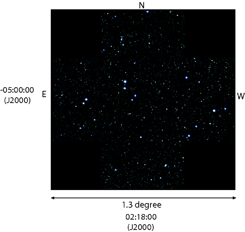
The optical imaging observations of the SXDF are carried out using the prime-focus camera (Suprime-Cam; Miyazaki et al. 2002) on Subaru Telescope in the period from September 2002 to September 2005. Suprime-Cam is a mosaic of ten MIT/LL buttable 2k4k CCD camera. It has a field of view with a projected pixel scale of 0.202 arcsec. The layout of the pointings is arranged as a cross shape so that each of the North-South and the East-West directions has an extent of deg (Figure 1). This corresponds to a field span of a transverse dimension of Mpc at and Mpc at in the comoving scale for (). The coverage of the comoving volume is Mpc3 for . Table 1 lists field center coordinates of the five pointings. Hereafter, the five pointings are referred to as (Center), (North), (South), (East), and (West), with respect to their relative positions on the sky.
Observations of the SXDF are performed using five broad-band filters, , , , , and to cover the entire wavelength range observable with Suprime-Cam. The transmission curves of the five filters employed in the SXDS, convolved with the CCD sensitivities, reflectivity of the primary mirror, transmissions of corrector lenses, and atmospheric transmission, are given in Figure 2. Also, given in Figure 2 are the redshifted spectral energy distributions (SEDs) of an early-type galaxy at and and a late-type galaxy at and for references. With photometric data sampled in the 5 bands, we can investigate color properties of red passively evolving galaxies to (see Kodama et al. 2004; Yamada et al. 2005) and young star-forming galaxies at high redshift such as lyman break galaxies (LBG) (Ouchi et al. 2004, 2005). The observations used in this paper span observing runs over a period of 3 years. A total of 160 hours are allocated to the SXDF imaging observations as a part of Subaru Telescope “Observatory Projects” (see also Kashikawa et al. 2004) combined with observatory staff times. In addition to these times, we use 14 hours of the observing times offered by the Supernova Cosmology Project (Doi et al. 2003; Lidman et al. 2005), which add the total exposure time of the center and the west pointings in the band (-C and -W). Moreover, in the course of another survey program for Ly emitting galaxies (Ouchi et al. 2005, 2007), 3 hours are devoted to the -band imaging. In total, 133 hours are used for on-source exposures for the final data set described in this paper. The complete log of the observations is given in Table 2.
The coordinates of the five pointings are carefully chosen so that the resultant images uniformly cover the entire SXDF, though we analyze each of the pointings separately in the present study. Also, to eliminate bad pixels, gaps between individual CCD chips and cosmic ray events, circular dithering pattern is used for each pointing. This dithering pattern employs a circular motion with radii of 60 to 120 arcsec around the center position of each pointing, combined with slight offsets to the center positions of the circular motion. As an example, the dithering pattern for the band is plotted for each pointing in Figure 3.
3 DATA REDUCTION
The SXDS images obtained are processed using an in-house pipeline software package (See Ouchi 2003). We use it in almost the same way that successfully used for the SDF (Kashikawa et al. 2004). This pipeline is based on a software package developed for Suprime-Cam data reduction (Yagi et al. 2002) and several IRAF tasks (geomap, geotran, etc.) are used in the process of a geometrical transformation and alignment of final stacked images. We use a standard mosaic-CCD data reduction procedure, which is briefly summarized below.
First, we apply a bias correction to the raw data. The median count of the overscan region is computed for each line, which represents a typical bias level at that line, and this median count is subtracted from the counts in all the pixels in that line. The overscan regions are trimmed after the bias subtraction. We assign a flag number (-32768) to the saturated or detected bad pixels, and these pixels are ignored in the following reduction processes. Since pixels in the outside edges of each frame are likely to be affected by noises which can not be corrected by the following flatfielding process, they are also masked with the flag number.
Flat frames are constructed from the normalized object frames taken during the same observing run. We use more than 150 object frames to create flat frames. If the number of object frames is less than 150 frames, object frames taken in different observing runs within 3 months or twilight flat frames taken in the same run are combined to increase the signal-to-noise ratios (S/Ns) of the flat frames for that period. The median value of the each pixel is used to create the flat frames. Pixels which could be affected by bright objects and vignetting by the auto-guider probe are flagged out before processing the flat frames. Then, object frames are divided by the flat frames. The peak-to-peak ratios of background levels over the entire flat fielded frames are less than . We do not expect any significant systematic errors by the flatfielding that affect accuracies of the following analyses.
After the flatfielding process is done, the distortion correction is applied to each frame using the 5-th order polynomial transformation formula derived from Miyazaki et al. (2002). The changes in shapes and sizes of objects in the frames due to the distortion are negligible compared with the size of PSFs. Each pixel is transformed so that the surface brightness of the pixel is conserved, since the relative flux in each pixel has been already corrected by the flatfielding process. Positional displacement of objects along the perpendicular orientation due to the atmospheric effect is also corrected at the same time.
The sky background is subtracted from each distortion-free frame, We divide an image into temporary meshes with pixels, corresponding to 12.9 arcsec in one direction. The mode of counts in each mesh is adopted as the sky background levels after smoothed by a median filter with a kernel. This global sky subtraction should not affect photometric accuracies of compact objects such as galactic stars and faint galaxies. However, caution must be taken when we apply these values to extended objects such as nearby galaxies with low surface brightness.
The stacking of the images is performed for each of the pointings separately in the following way. First, we choose 100 to 200 unsaturated stellar objects with a peak flux of ADU in each frame distributing evenly over the entire frame. Second, we determine a reference frame of all the reduced frames. For the other frames, relative positions and rotation () and flux ratios to the reference frame are determined based on a least square method using these stellar objects commonly detected in the frames. Third, for all the frames, the positional shifts and rotations are corrected. Here, we do not use frames which have the flux ratios of less than of that of the reference frame. Finally, all the frames are co-added by calculating flux-weighted average values in each pixel with a 3- clipping process. The clipping process effectively removes cosmic rays and bad or saturated pixels, and satellite trails etc., and should not affect the resulting total fluxes of objects because the difference in counts among frames with various seeing sizes is mostly within the 3- threshold.
After the co-adding of each band images, all the five-band () images are registered into identical positional coordinates as we intend to execute multi-waveband aperture photometry. The positional registration is performed by the geometrical transformation by 3-rd order polynomials fitting using the positions of stellar objects common to the co-added stacked images. The r.m.s. deviation of residuals of transformed positions with respect to the reference positions in the -band images is approximately 0.1-0.15 arcsec.
For each pointing, the geometrically matched images are smoothed with Gaussian filters iteratively so that the PSF sizes of all the images become the same as that in the worst image used in this study. The PSF sizes of the resultant images are , and arcseconds in SXDS-C, SXDS-N, SXDS-S, SXDS-E, and SXDS-W, respectively.
Finally, regions with low S/Ns or those affected by saturation or overflow of electrons are carefully checked and assigned as flagged regions which are indicated in photometric catalogs. The resultant PSF sizes and total usable areas of each pointing is summarized in Table 3.
4 MULTI-WAVEBAND PHOTOMETRIC CATALOGS
We construct multi-waveband photometric catalogs of the objects identified in the SXDF.
4.1 Object Detection
Object detection and photometry are performed using SExtractor version 2.3.2 (Bertin & Arnouts 1996). Before performing the object detection and photometry, the outskirts of the stacked images are trimmed in order to eliminate any failure such as inappropriate estimation of sky levels and memory overflow during extraction of objects by SExtractor due to a high noise level. After trimming the outskirts, each individual image has similar size of approximately pixels. We use the detection criteria that at least five pixels which have values of of sky background r.m.s. noise must be connected in order to be included in our object list. Positions of detected objects are translated to sky coordinates based on the astrometric calibration which will be discussed in Section 5.2.
4.2 Aperture Photometry
After the object detection is completed in one of the five bands, which we call ‘detection band’, multi-waveband aperture photometry is carried out with SExtractor for the other four bands using the same apertures at the same positions as those in the detection band. We perform aperture photometry with fixed circular apertures (MAG_APER) of and arcseconds in diameter, and variable elliptical apertures (MAG_AUTO and MAG_BEST) utilizing the Kron’s first moment scheme with apertures’ radii of (Kron 1980). Measured fluxes of objects are converted into magnitude using the photometric zeropoints, which will be described in Section 5.1. The extracted magnitude is considered to be the asymptotic total magnitude of galaxies, which should sample at least of flux of a galaxy (Bertin & Arnouts 1996). Other useful parameters for objects including shape, size, and stellarity and so on, are also extracted by SExtractor at the same time. All the object parameters which are listed in the catalogs are summarized in Table 4.
In this procedure, -, -, -, -, and -selected multi-waveband catalogs are created for each pointing separately, which means that each object has measurements in the five bands () in each catalog. Thus 25 catalogs (= 5 pointings times 5 detection bands) in total are created.
4.3 Flagged Areas
Although we have flagged out bad pixels from the image frame in the reduction procedure, there still remain (1) areas strongly affected mainly by overflow of electrons or envelopes of extended objects, and (2) areas weakly affected by large halos from very bright stars or noisy regions. In our catalogs, the objects which are located in these areas are flagged 1 and 2, respectively. Otherwise, the objects located in the clean area have a flag value of 0.
The basic parameters used in the object detection and aperture photometry are summarized in Table 5. The complete configuration files for SExtractor can be found at http://www.naoj.org/Science/SubaruProject/SXDS/index.html. Note that we adopt default parameters of SExtractor for the source extraction unless we do not find any problem with the output values. The parameters adopted are suitable for extraction of moderate to faint compact galaxies, and not heavily optimized to extraction of extended objects or very faint objects. Thus the reliability of the current catalogs for those objects should be regarded with some caution.
5 CALIBRATIONS
5.1 Photometric Calibration
Photometric zeropoints in all the five bands are determined in the following way. First, we compare our observation with the earlier calibrated observations for the same overlapping field, which were made by the Suprime-Cam instrument development team (Ouchi et al. 2001, 2004). The southern half of our center pointing (SXDS-C) is overlapped with the northern half of the image obtained by Ouchi et al. (2001). They determined the photometric zeropoints in the Suprime-Cam band system based on observations of photometric standard stars SA92 and SA95 for and bands and a spectrophotometric standard star SA95-42 for and bands.
We estimate the photometric zeropoints for our center pointing (SXDS-C) by comparing magnitudes (MAG_AUTO) of objects which are commonly detected in the two images and have FWHMs of smaller than 1.2 arcsec with a magnitude range of 20.0 to 24.0. Then, we extend these zeropoints to the surrounding four pointings by using objects in the overlapping areas in the same manner as for the determination of the zeropoint for the SXDS-C. In our catalogs, we list the instrumental magnitude obtained in the Suprime-Cam band system. Hence, no transformation of magnitude considering color terms of band responses are conducted. The color terms between the Suprime-Cam band system and the standard system are basically small – for the reddest stars, of order 0.1 in the bands, and slightly large () in the band.
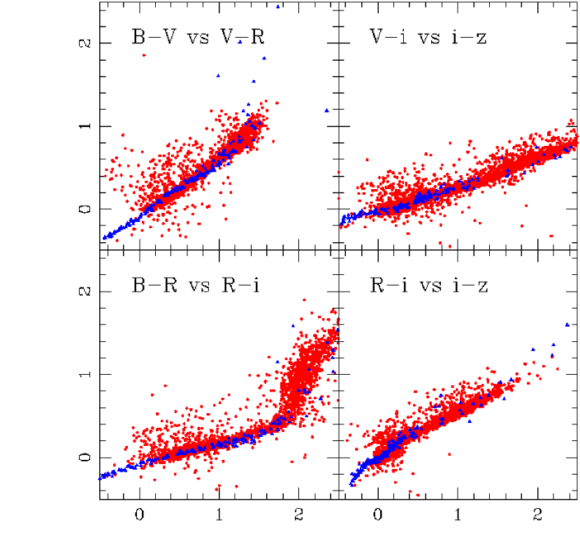
To test internal consistency of our zeropoint calibrations, we examine colors of stellar objects in our photometric catalogs and those computed by convolving typical stellar SEDs covering the complete ranges of spectral types (Gunn & Stryker 1983) with Suprime-Cam response curves. We find that it is necessary to apply corrections to the zeropoints of and for all the five pointings, and and for the South and East pointings (-S and -E), respectively. After these corrections are applied, the colors of the stellar objects in our catalogs agree with those computed for the SEDs from Gunn & Stryker (1983) within mag in all the five bands (Figure 4). The systematic errors adjusted here may be due to relatively small number of stellar objects used in the determination of the photometric zeropoints.
To ensure the accuracy of our zeropoints, we conduct CCD photometric observations of a part of the SXDF in and bands with the UH88-inch telescope at Mauna Kea on October 9 and 10, 2002. We compare magnitudes of objects in and bands obtained by the UH88-inch observations with our catalog values. We find that our catalog values agree within 0.05 mag r.m.s. for and bands and within 0.1 mag r.m.s. for and bands. The relatively large difference seen in and bands are probably due to the difference in the band responses between the UH88-inch system and the Suprime-Cam system, and low S/Ns of shallow SXDS images used for comparison with the UH88-inch data. To confirm accuracy of the photometric zeropoints in the and bands in our catalogs, follow-up observations are made for the two bands with the 1.0-m telescope at the United States Naval Observatory (USNO). The observations at the USNO were performed on the photometric night of December 3, 2004 in the course of photometric calibration for a high- supernovae search (Yasuda et al. 2007, in preparation). We find that a systematic difference between zeropoints in our catalogs and those determined by the USNO observation is as small as mag r.m.s.
Thus we conclude that the uncertainties of calibrated photometric zeropoints of the SXDS images are mag r.m.s. The adopted photometric zeropoints are listed in Table 2.
5.2 Astrometric Calibration
Astrometric calibration is performed using 200 stars with magnitude of derived from 2-MASS point source catalogs (PSC; Cutri et al. 2003), in each of the five stacked -band images. Since images in the other bands have been geometrically transformed, the positions of objects detected on the images should coincide with those found in the -band images (see Section 3). The world coordinates for the images are calculated for the -band images and written in the FITS headers of all the stacked images with the IRAF tasks CCMAP and CCSETWCS. The r.m.s. uncertainties of the determined coordinates across the FOV with respect to the PSC positions are on the order of 0.2 arcsec in both RA and Dec in each pointing (Table 6). The positional error of the PSC is reported as arcsec.
We examine possible systematic differences in the calculated world coordinates between different pointings by using objects in the overlapping areas of two pointings. Figure 5 and Figure 6 show the differences in RA and Dec of point-like objects with FWHMs arcsec in the magnitude range detected both in the SXDS-C image and other surrounding images. From the figures, the world coordinates assigned to each of the five pointing images are in good agreement with one another with accuracy of about 1 arcsec at the edges of the images. The differences of the world coordinates between two pointings studied here are thought to be for the worst cases, since they are derived based on only the objects in the overlapping areas which are located at the edge of each image. Slopes and offsets in the residuals are seen in each panel of the figures. These disagreements in the positions of objects between two overlapping images come from possible tilts, offsets and/or difference in geometrical scale of the world coordinate systems between the two images. Residuals of distortion in the images and the atmospheric effect, which have not been completely removed in the reduction process, may cause the errors in determination of the world coordinate systems. Nevertheless, the SXDS catalogs have a good enough positional accuracy to perform follow-up spectroscopy.
The astrometrically and photometrically calibrated images of the SXDS in five bands ( ) described in this section are released via SXDS Web Page (http://www.naoj.org/Science/SubaruProject/SXDS/). The data set described in this paper is based on the data release 1 (DR1). A complete history of the data release is summarized in the web site. The raw image data are also available to the public via Subaru Telescope ARchives System (STARS: https://stars.naoj.org).
6 PROPERTIES OF THE CATALOGS
6.1 Galactic Extinction
All the magnitudes listed in the catalogs are not corrected for the Galactic extinction. The magnitude attenuation in each band estimated for the central position (; J2000) based on Schlegel et al. (1998), assuming an extinction curve with is as follows: , and . Table 7 summaries the magnitude attenuation in each band for all the pointings. The Galactic extinction above must be taken into account when studying extragalactic objects.
6.2 Limiting Magnitudes
We examine 3- limiting magnitudes measured for the -diameter apertures in all five bands ( column in Table 2) in the following manner. First, counts in unit of ADU fallen into the -diameter apertures are measured at approximately 10,000 positions randomly selected and spreading over the entire image. Next, a histogram of the counts is produced and only the faint side of the histogram is fit by the Gaussian function, as the bright-side tail is composed of not only the sky background but also photons from the objects. The of the best-fit Gaussian is regarded as the 1- sky fluctuation of the image for the -diameter apertures. We find that limiting magnitude in each band is and () in the deepest images of the five pointings.
6.3 S/N Distribution Map
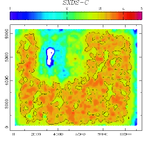
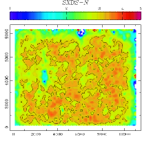
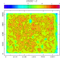
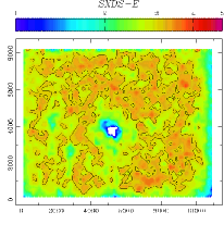
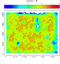
To examine the homogeneity of S/Ns of the SXDS data across the entire field, we investigate the S/N distribution map in the -band images. First, we calculate the sky fluctuation per -diameter aperture within a mesh with a size of pixels at each position in the same manner as in estimation of the limiting magnitudes. The mesh is shifted with a step of 175 pixels to cover the entire field of view. Then, the fluctuations for the 2”-diameter aperture are converted to S/Ns for objects with an magnitude of 27.5 at each position.
Figure 7 shows the S/N distribution maps for 27.5-mag objects thus obtained for each pointing. The contour lines superimposed on the figures represent S/N=3 positions. First, we see that the brightest sources on the images significantly affect the S/Ns around the sources. These areas are flagged in the catalogs. Second, each image shows almost an axisymmetric pattern of the S/N distribution when we ignore the low S/N areas due to the brightest sources. This pattern reflects the vignetting of the prime focus. Third, the pattern is slightly distorted for each image, probably due to bright sources, vignetting by the auto-guider probe, difference in the quantum efficiency among CCDs, and so on. However, the difference in S/Ns between in such distorted areas and in clean areas with higher S/Ns is on the order of 20% at the maximum. This difference is negligible in most studies even for faint sources. Thus, we can securely utilize the data with quite homogeneous S/Ns across the field of view.
6.4 Completeness and False Detection Rate
Completeness of the object detection as a function of magnitude for each band and for each pointing is estimated. The detection completeness is determined based on a Monte Carlo simulation by adding artificial objects which have Gaussian profiles with their Poisson photon noise into a stacked image used to create the catalogs and then detect them again in the same manner as in creating catalogs. The detection rate thus obtained is regarded as the detection completeness. Here the artificial objects are added to random positions in the effective area of the image. The FWHMs of the Gaussian profiles are set to be the same as the PSF sizes representative of the images which are derived from Table 3. The artificial objects contaminated by any neighbor sources listed in the catalogs are removed in calculation of the detection rate. If such blended objects are not removed from the sample, the detection rate should slightly decrease. However, since the contamination by neighbor objects leads to misidentification of the artificial objects in the object detection process, we adopt the approach which excludes the blended artificial objects, which was also employed in Kashikawa et al. (2004).
The completeness determined by this procedure is shown in Figure 8 for all of the five bands. For the five pointings, the curves of the detection completeness drop similarly with increasing magnitude. We can summarize that the detection completeness in each image is at approximately for objects with the 5- magnitude and for objects with the 3- magnitude, with a slight difference depending on the band.
On the other hand, rates of the false object detection are also estimated as a function of magnitude. We generate negative images of each pointing and in each band by multiplying all the counts of the stacked images by , and then perform object detection for the negative images in the same manner as in creating the catalogs. In this process, detected objects are considered to be spurious objects. Thus we define the false detection rate as the number of the spurious objects divided by the total number of objects in the catalogs in each magnitude bin, i.e., (Figure 9). It is seen that a contribution of the false detection is negligible, which does not exceed 0.5% if any, in the magnitude range brighter than the 3- limiting magnitude.
6.5 Magnitude Differences among the Catalogs
In the areas where two images overlap with each other, a large fraction of objects are detected and their magnitudes are measured in both of the pointings. We can check systematic difference in magnitude of those objects between the two catalogs. Since photometric zeropoints of the catalogs are determined so that MAG_AUTO of objects in the overlapping areas should coincide between any two catalogs (see Section 5.1), the magnitude difference in MAG_AUTO is negligible. MAG_BEST should be identical to MAG_AUTO for isolated objects. Therefore magnitude differences only for the - and -diameter aperture magnitudes are investigated in the following manner.
First, we choose only compact objects with FWHMs arcsec which are listed in both the -selected catalog for SXDS-C and that for another pointing which overlap with each other, then measure the difference in magnitude of the objects by subtracting magnitude in the SXDS-C catalog by that in the other. Then, we determine the offset in the magnitude difference, i.e., systematic magnitude difference, by fitting the magnitude difference for a range of 21.0 to 23.5 mag by a least square method. Table 8 lists the systematic magnitude difference thus obtained for the - and - diameter aperture magnitudes in each band for each pair of catalogs. We note that - and -diameter aperture magnitudes indicate small systematic differences of mag between the catalogs. We think that this difference is probably due to difference in the PSF shape of the stacked images among the pointings.
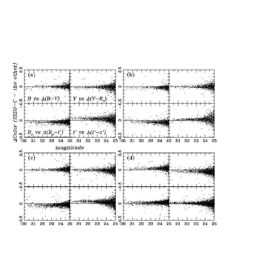
In order to see the effects of the systematic difference in the aperture magnitudes, we plot differences in colors of objects between the catalogs measured with the -diameter aperture magnitude (Figure 10). In this figure, for each of the four pairs of catalogs, the differences in colors () are plotted. We see the systematic difference in the -diameter aperture colors of objects, which is no larger than mag, due to the difference in the aperture magnitude between the catalogs. Since the magnitudes in the catalogs are not adjusted for this difference, the magnitude difference between the catalogs should be taken into account in the case that the - or -diameter aperture magnitude is used. For MAG_AUTO and MAG_BEST, which are considered as asymptotic total magnitude, the magnitude difference is negligible.
In the same manner as mentioned above, the r.m.s. of the magnitude differences for each band are calculated as a function of MAG_AUTO, which shows no systematic difference. Here the detection band for catalogs are chosen to be the same as the band for which the magnitude difference is investigated. For instance, to obtain the magnitude difference in the band, the -selected catalogs are used. Again, only the objects with FWHMs arcsec are used for measurement of the magnitude difference. The r.m.s. of magnitude differences measured in the above way are shown in Figure 11 for each band. It is seen that the r.m.s. steadily increases with increasing magnitude. The r.m.s. of the magnitude difference can be converted into random magnitude error by dividing it by . We find that the magnitude errors thus estimated are entirely consistent with those expected from our calculation of the limiting magnitude discussed in Section 6.2. Note that the magnitude errors listed in our catalogs are computed by SExtractor assuming the simple Poisson statistics for the sky background fluctuations. The sky background noises measured in photometry apertures for the stacked images are likely to be larger than those estimated by SExtractor. Therefore the magnitude errors in the catalogs are underestimates and are not suitable for immediate analysis such as SED fitting and photo- estimation.
6.6 Number Counts of Galaxies
To examine the characteristics of the catalogs we compare the number counts of galaxies with data from previous surveys.
We calculate the number counts of galaxies by correcting our raw counts of detected objects against the detection completeness estimated in Section 6.4. The detailed studies of density fluctuations of galaxies based on the number counts or luminosity functions of galaxies can be found in elsewhere (e.g., Yamada et al. 2005). Star/galaxy separation is conducted based on FWHM and -diameter fixed aperture magnitude of the objects, for which the effect of the Galactic extinction (Table 7) is corrected. The criteria for the separation is determined so that both objects which have sizes as same as PSF of the images and saturated objects are effectively removed. For fainter magnitudes ( mag), no separation is performed since a large fraction of galaxies have small sizes similar to those of stars, and contribution to the number count by stars is small at the faint magnitudes. The criteria for the separation adopted is summarized in Table 9.
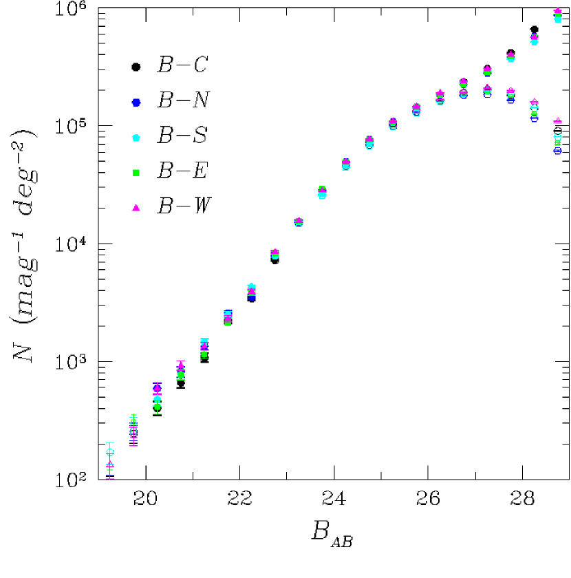
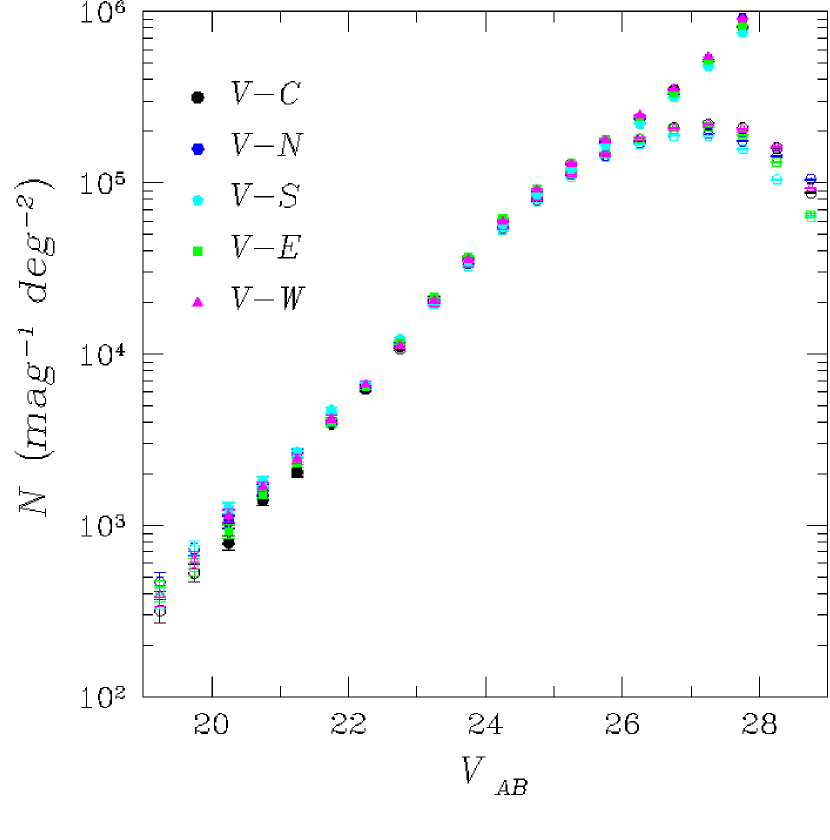
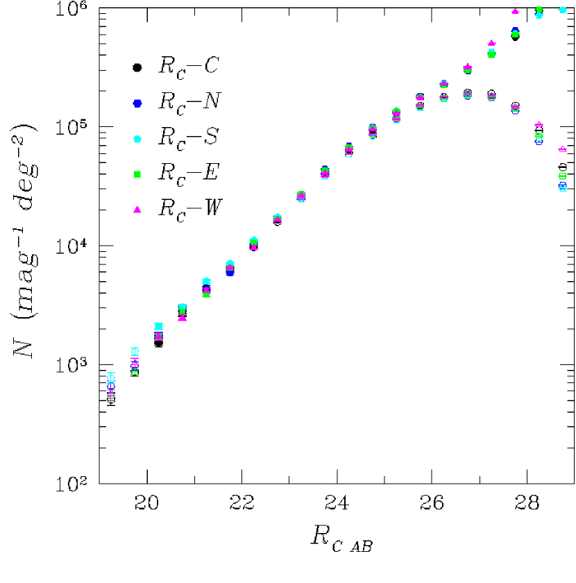
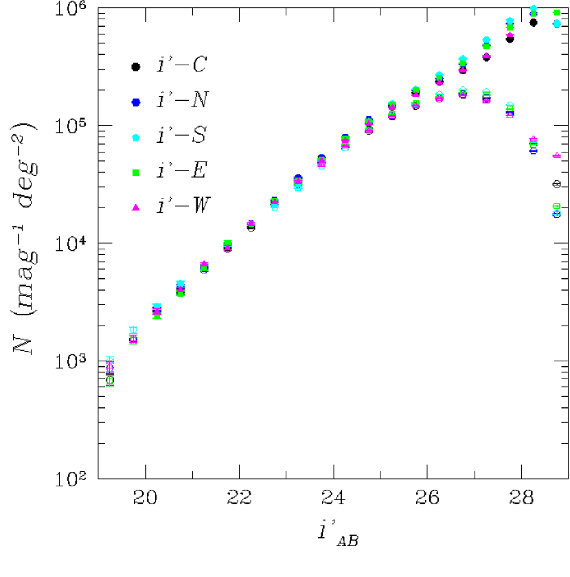
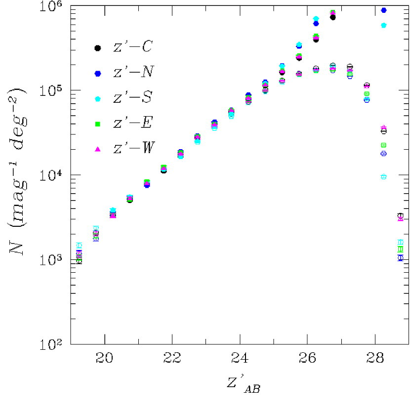
The results of the number counts of galaxies are as follows: First, internal comparison of the number counts among the five pointings of the SXDS are shown for each band in Figure 12 to Figure 16. In each figure, raw number counts of the galaxy samples extracted by the star/galaxy separation process above are plotted with open symbols. Effective areas used to calculate the number counts per unit area are given in Table 3. The number counts of galaxies which are corrected for the detection completeness are also superimposed with filled symbols. Here, the correction is performed by using the detection completeness as a function of magnitude which has been estimated for the Gaussian profiles, i.e., . Error bars are calculated on the assumption of simple Poisson noise. We can say that no large systematic difference is seen in the superposition of the number counts of galaxies among the five pointings in , and bands down to the 3- magnitudes. Similarly, in the other two bands, the number counts are consistent with one another among the five pointings within the Poisson errors at magnitudes brighter than mag. However, differences in the number counts at fainter magnitudes are found by a factor of 1.4 in the band and 1.7 in the band. This might be partly due to the field-to-field variation in the number counts of galaxies. However, since we have used only the Gaussian profiles with FWHM arcsec in the simulation of the detection completeness, the completeness is likely to be overestimated at a faint magnitude range where most objects have extended profiles. So, we cannot conclude that the differences in the number counts at the faint end seen in the and bands indicates the field-to-field variation.
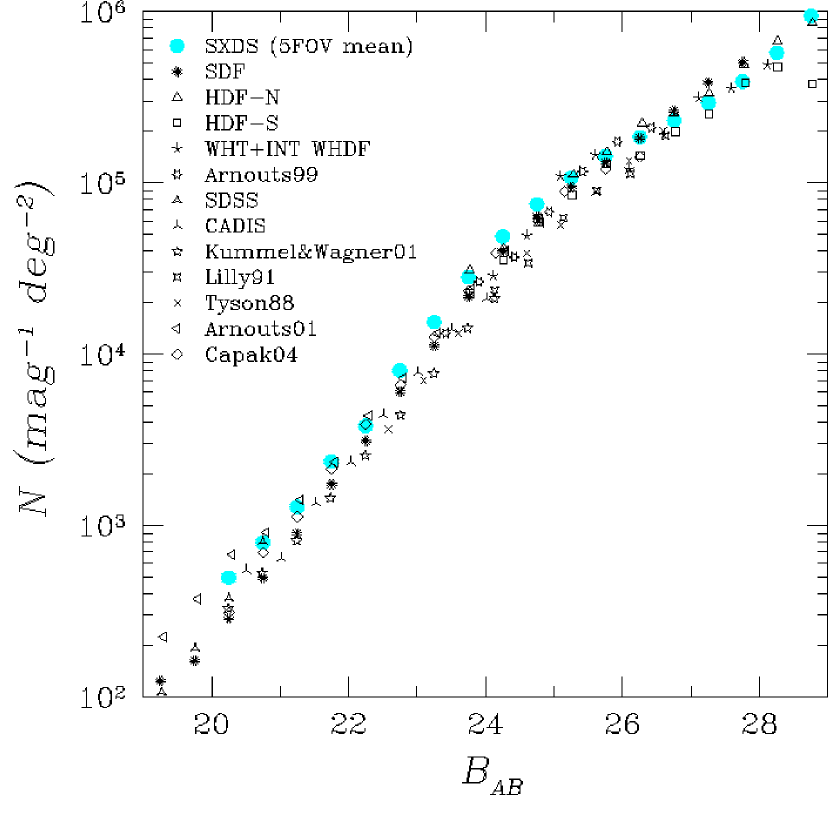
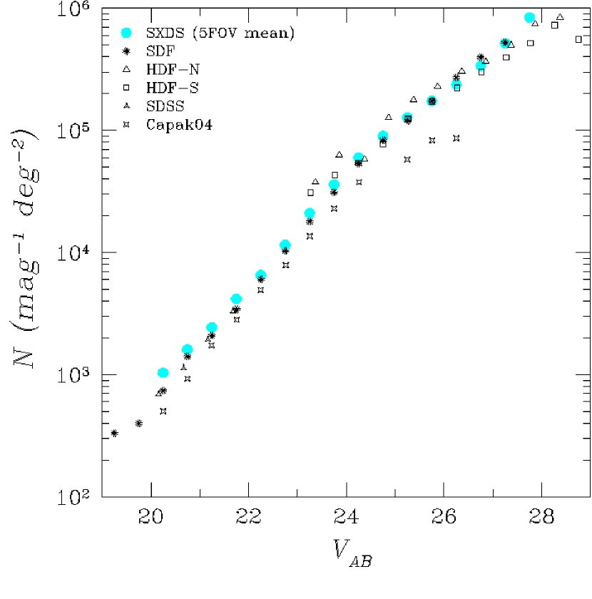
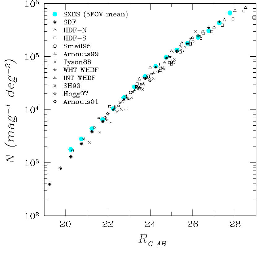
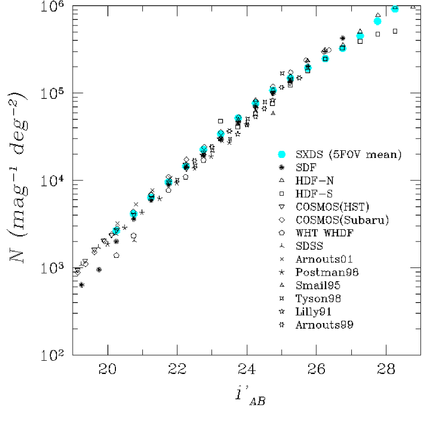
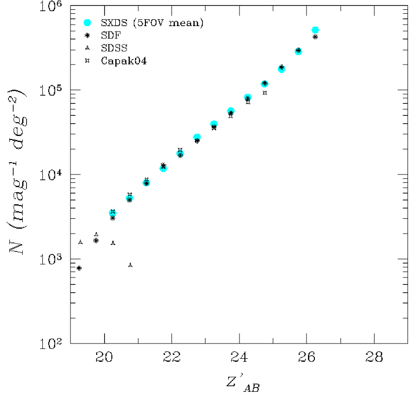
Next, the number counts in the SXDF are compared with results by previous surveys (Figure 17 to Figure 21). Here, we calculate mean number counts of galaxies corrected for the detection completeness for the entire SXDF using the above sample for the five pointings, and plot them with filled circles with error bars. The error bars are again based on the Poisson noise. The results in other surveys are derived from Kashikawa et al. (2004), Capak et al. (2007), and Metcalfe (2007)222http://star-www.dur.ac.uk/~nm/pubhtml/counts/counts.html and the references cited therein. A complete list of references compared in the figures is as follows: SDF – Kashikawa et al. 2004, HDFs/WHDFs – Metcalfe et al. 2001, Arnouts99 – Arnouts et al. 1999, SDSS – Yasuda et al. 2001, CADIS – Huang et al. 2001, Kummel&Wagner01 – Kümmel & Wagner 2001, Tyson88 – Tyson 1988, Arnouts01 – Arnouts et al. 2001, Capak04 – Capak et al. 2004, Smail95 – Smail et al. 1995, SH93 – Steidel & Hamilton 1993, Hogg97 – Hogg et al. 1997, COSMOS – Capak et al. 2007, Postman98 – Postman et al. 1998, Lilly91 – Lilly, Cowie, & Gardner 1991.
From the comparison of the number counts among various surveys, we understand that our sample is consistent with results in other surveys for blank fields for the following reasons. First, the mean number counts of the SXDS show a good agreement with those from previous surveys down to magnitude where the number counts start to turn off. Second, it reproduces the faint-end data points derived from Hubble Deep Field (HDF). Again, the detection completeness simulated with the Gaussian profiles might cause a slightly large uncertainty of the corrected number counts at the faint end in each band. Thus, we conclude that the SXDS catalogs in the present study have characteristics similar to those in previous surveys and can be applied to general statistical studies on faint objects ranging from Galactic objects to high-redshift galaxies.
We would like to mention how the Poisson error on the number counts is decreased by increase of the survey area. Figure 22 shows a comparison of the Poisson error associated with the number counts of galaxies among three surveys which are based on different survey areas, namely the HDF-North (5.3 arcmin2), GOODS-North (170 arcmin2) and Suprime-Cam 1 FOV (918 arcmin2). The uncertainty in the number counts due to the Poisson error is shown with a pair of lines for each of the surveys. For reference, the number count of SXDS is superimposed with a thick solid line. From the figure, we clearly see that the Poisson error decreases with increasing survey area. In particular, at the bright magnitudes of mag, a large uncertainty by a factor of in the number count is found for the HDF-North area (dotted lines). For the same magnitude range, the uncertainty for a field of view of Suprime-Cam (dot-and-dash lines) is times as small as that for the HDF-North area and times as small as that for the GOODS-North area. Even at the faintest magnitudes of mag, a significant difference in the uncertainty from one to another survey area is seen. Thus it is emphasized that the SXDS data, which consists of five pointings of Suprime-Cam field of view, is a useful data set for studies on celestial objects which dominate a large fraction of the number counts without suffering from the Poisson error and the field-to-field variation as well, e.g., a study of evolution of the LSSs.
7 SUMMARY
The optical imaging observations of the SXDS project are carried out using the Suprime-Cam on Subaru Telescope in and bands. The SXDF has a contiguous area coverage of 1.2 deg2, which consists of five Suprime-Cam pointings.
The photometric zeropoints are determined with an absolute accuracy of no larger than 0.05 mag r.m.s. in the photometry. The r.m.s. of the astrometric accuracies across the field is on the order of 0.2 arcsec in both RA and Dec. The systematic differences in the adopted world coordinates between different pointings are within about 1 arcsec at the outer edge of the field of view. Thus, our SXDS catalogs have a good enough positional accuracies to perform follow-up spectroscopy.
Multi-waveband photometric catalogs of detected objects are created for each band and for each pointing. Each of the catalogs contains more than a hundred sixty thousand of objects. The catalogs have quite homogeneous S/Ns across the field. The achieved limiting magnitudes in each band are and ().
The detection completeness as a function of magnitude is estimated by a Monte-Carlo simulation assuming a Gaussian profile. The number counts of galaxies in the SXDF in each band are computed by correcting the detection completeness, which are consistent with each other among the five pointings with a slight difference at faint magnitudes. The mean number counts of galaxies averaged over the five pointings show a good agreement with results from previous surveys down to the faint-end magnitude.
With the aid of the wide coverage area of SXDS data, the uncertainty of the number counts of galaxies due to the Poisson error is greatly decreased. It is emphasized that the SXDS data is extremely useful for pursuing studies on celestial objects spreading in a wide field without suffering from the Poisson error and the field-to-field variation. The SXDS catalogs can be applied to studies, scientific objectives of which range from the Galactic objects to the large scale structures of the universe.
The optical data, the compiled photometric catalogs, and configuration files used to create the catalogs have been released to the public and can be retrieved from the public data archives server of National Astronomical Observatory of Japan, http://www.naoj.org/Science/SubaruProject/SXDS/index.html.
Acknowledgments
We thank Dr. Masafumi Yagi for his kind suggestions in analyzing the data based on the software package developed by himself. We thank Dr. Nobunari Kashikawa for fruitful discussions. The anonymous referee would also be appreciated for his/her constructive suggestions. We would like to convey our gratitude to the Subaru Telescope builders and staff for their invaluable help to complete the observing run with Suprime-Cam. Data reduction/analysis in this work was in part carried out on ”sb” computer system operated by the Astronomical Data Center (ADC) and Subaru Telescope of the National Astronomical Observatory of Japan. Use of the UH 2.2-m telescope for the observations is supported by NAOJ.
References
- Arnouts et al. (1999) Arnouts, S., D’Odorico, S., Cristiani, S., Zaggia, S., Fontana, A., & Giallongo, E. 1999, A&A, 341, 641
- Arnouts et al. (2001) Arnouts, S. et al. 2001, A&A, 379, 740
- Bertin & Arnouts (1996) Bertin, E. & Arnouts, S. 1996, A&AS, 117, 393
- Bolzonella et al. (2000) Bolzonella, M., Miralles, J.-M., Pelló, R. 2000, A&A, 363, 476
- Capak et al. (2004) Capak, P. et al. 2004, AJ, 127, 180
- Capak et al. (2007) Capak, P. et al. 2007, ApJS, 172, 99
- Coppin et al. (2006) Coppin, K. et al. 2006, MNRAS, 372, 1621
- Cutri et al. (2003) Cutri, R. M. et al. 2003, VizieR On-line Data Catalog: II/246 (Originally published in University of Massachusetts and Infrared Processing and Analysis Center (IPAC/California Institute of Technology))
- Dye et al. (2006) Dye, S. et al. 2006, MNRAS, 372, 1227
- Doi (2003) Doi, M. et al. 2003, IAU Circ., 8119, 1
- Feldmann et al. (2006) Feldmann, R. et al. 2006, MNRAS, 372, 565
- Foucaud et al. (2007) Foucaud, S. et al. 2007, MNRAS, 376, L20
- Furusawa et al. (2000) Furusawa, H., Shimasaku, K., Doi, M., & Okamura, S. 2000, ApJ, 534, 624
- Giavalisco et al. (2004) Giavalisco, M. et al. 2004, ApJ, 600, L93
- Gunn & Stryker (1983) Gunn, J. E. & Stryker, L. L. 1983, ApJS, 52, 121
- Hogg et al. (1997) Hogg, D. W., Pahre, M. A., McCarthy, J. K., Cohen, J. G., Blandford, R., Smail, I., Soifer, B. T. 1997, MNRAS, 288, 404
- Huan et al. (2001) Huang, J.-S. et al. 2001, A&A, 368, 787
- Kashikawa et al. (2004) Kashikawa, N. et al. 2004, PASJ, 56, 1011
- Kodama et al. (2004) Kodama, T. et al. 2004, MNRAS, 350, 1005
- Kron (1980) Kron, R. G. 1980, ApJS, 43, 305
- Kummel & Wagner (2001) Kümmel, M. W. & Wagner, S. J. 2001, A&A, 370, 384
- Lawrence et al. (2007) Lawrence, A. et al. 2007, MNRAS, 379, 1599
- Lidman et al. (2005) Lidman, C. et al. 2005, A&A, 430, 843
- Lilly et al. (1991) Lilly, S. J., Cowie, L. L., & Gardner, J. P. 1991, ApJ, 369, 79
- Lonsdale et al. (2003) Lonsdale, C. J. et al. 2003, PASP, 115, 897
- Metcalfe et al. (2001) Metcalfe, N., Shanks, T., Campos, A., McCracken, H. J., & Fong, R. 2001, MNRAS, 323, 795
- Miyazaki et al. (2002) Miyazaki, S. et al. 2002, PASJ, 54, 833
- Mortier et al. (2005) Mortier, A. M. J. et al. 2005, MNRAS, 363, 563
- Ouchi et al. (2001) Ouchi, M. et al. 2001, ApJ, 558, L83
- Ouchi (2003) Ouchi, M. 2003, PhD thesis, University of Tokyo
- Ouchi et al. (2004) Ouchi, M. et al. 2004, ApJ, 611, 660
- Ouchi et al. (2005) Ouchi, M. et al. 2005, ApJ, 620, L1
- Ouchi et al. (2007) Ouchi, M. et al. 2007, ArXiv e-prints, 707, arXiv:0707.3161
- Postman et al. (1998) Postman, M., Lauer, T. R., Szapudi, I., & Oegerle, W. 1998, ApJ, 506, 33
- Schlegel et al. (1998) Schlegel, D. J., Finkbeiner, D. P., & Davis, M. 1998, ApJ, 500, 525
- Scoville et al. (2007) Scoville, N. et al. 2007, ApJS, 172, 38
- Simpson et al. (2006) Simpson, C. et al. 2006, MNRAS, 372, 741
- Smail et al. (1995) Smail, I, Hogg, D. W., Yan, L., & Cohen, J. G. 1995, ApJ, 449, L105
- Steidel & Hamilton (1993) Steidel, C. C. & Hamilton, D. 1993, AJ, 105, 2017
- Tyson (1988) Tyson, J. A. 1988, AJ, 96, 1
- Ueda et al. (2007) Ueda, Y. et al. 2007, ApJS, submitted
- Yagi et al. (2002) Yagi, M., Kashikawa, N., Sekiguchi, M., Doi, M., Yasuda, N., Shimasaku, K., & Okamura, S. 2002, AJ, 123, 66
- Yamada et al. (2005) Yamada, T. et al. 2005, ApJ, 634, 861
- Yasuda et al. (2001) Yasuda, N. et al. 2001, AJ, 122, 1104


| Pointing | RA (J2000) | Dec (J2000) | Position Angle of FOV |
|---|---|---|---|
| Center | North is up | ||
| North | North is up | ||
| South | North is up | ||
| East | East is up | ||
| West | West is up |
Note. — Field names for each pointing and their positional coordinates. PA, the orientation of the FOV on the sky are chosen so that the overhead time to rotate the position angle are minimized and effective area with high signal-to-ratios are is maximized.
| Exp. Time | PSF Size | Zeropts for Images | ||||
|---|---|---|---|---|---|---|
| Band-Pointing | (min) | (arcsec) | (magABADU-1) | (magAB) | Date of Observations | |
| -C | 345 | 0.80 | 34.723 | 28.09 | 197,317 | 2002, Sep. 29/30, Oct. 01 |
| 2003, Nov. 17 | ||||||
| -N | 330 | 0.84 | 34.701 | 28.39 | 176,372 | 2002, Nov. 02/05/27, Dec. 01/07 |
| 2003, Nov. 17 | ||||||
| -S | 330 | 0.82 | 34.706 | 28.33 | 189,916 | 2002, Nov. 02/04/05/27, Dec. 01/07 |
| 2003, Nov. 17 | ||||||
| -E | 330 | 0.82 | 34.698 | 28.06 | 179,478 | 2002, Nov. 04/05, Dec. 01/07 |
| 2003, Nov. 17 | ||||||
| -W | 330 | 0.78 | 34.716 | 28.21 | 197,770 | 2002, Nov. 04/05/27, Dec. 01/07 |
| 2003, Nov. 17 | ||||||
| -C | 319 | 0.72 | 33.639 | 27.78 | 213,851 | 2003, Oct. 02/24/26 |
| 2004, Jan. 16, Oct. 09, Dec. 10/14/15 | ||||||
| 2005, Jan. 05 | ||||||
| -N | 313 | 0.80 | 33.648 | 27.65 | 203,299 | 2003, Oct. 02/26, Nov. 17 |
| 2004, Jan. 16, Dec. 10/14/15 | ||||||
| 2005, Jan. 05, Sep. 28 | ||||||
| -S | 321 | 0.82 | 33.643 | 27.75 | 186,545 | 2003, Oct. 02/24/26 |
| 2004, Jan. 16, Dec. 10/14/15 | ||||||
| 2005, Jan. 05, Sep. 28 | ||||||
| -E | 291 | 0.76 | 33.639 | 27.77 | 192,951 | 2003, Oct. 02/26 |
| 2004, Jan. 16, Dec. 10/14/15 | ||||||
| 2005, Jan. 05, Sep. 28 | ||||||
| -W | 293 | 0.72 | 33.649 | 27.72 | 205,915 | 2003, Oct. 02/26, Nov. 17 |
| 2004, Jan. 16, Dec. 10/14/15 | ||||||
| 2005, Jan. 05, Sep. 28 | ||||||
| -C | 248 | 0.76 | 34.315 | 27.57 | 188,079 | 2002, Sep. 30, Oct. 01/07 |
| 2003, Nov. 17 | ||||||
| -N | 232 | 0.78 | 34.276 | 27.74 | 174,365 | 2002, Nov. 01/09/30, Dec. 06 |
| 2003, Nov. 17 | ||||||
| -S | 232 | 0.74 | 34.219 | 27.67 | 178,416 | 2002, Nov. 01/09/30, Dec. 06 |
| 2003, Nov. 17 | ||||||
| -E | 232 | 0.76 | 34.259 | 27.51 | 173,586 | 2002, Nov. 02/09/30, Dec. 06 |
| 2003, Nov. 17 | ||||||
| -W | 232 | 0.82 | 34.247 | 27.53 | 186,648 | 2002, Nov. 02/09/30, Dec. 06 |
| 2003, Nov. 17 | ||||||
| -C | 647 | 0.78 | 34.055 | 27.62 | 181,352 | 2002, Sep. 29/30, Nov. 01/02/05/09/27/29, Dec. 06/07 |
| 2003, Oct. 20/21 | ||||||
| -N | 440 | 0.76 | 34.042 | 27.66 | 176,394 | 2002, Sep. 29/30, Nov. 01/02/09/29, Dec. 07 |
| 2003, Sep. 22, Oct. 02/21 | ||||||
| -S | 309 | 0.68 | 34.046 | 27.47 | 187,791 | 2002, Sep. 29/30, Nov. 01/02/09/29 |
| 2003, Sep. 22, Oct. 02 | ||||||
| -E | 368 | 0.74 | 33.986 | 27.49 | 175,404 | 2002, Sep. 29/30, Nov. 01/02/09/29, Dec. 07 |
| 2003, Sep. 22, Oct. 02/21 | ||||||
| -W | 598 | 0.82 | 34.087 | 27.58 | 178,543 | 2002, Sep. 29/30, Nov. 01/02/05/09/27/29, Dec. 06/07 |
| 2003, Oct. 20/21 | ||||||
| -C | 217 | 0.70 | 33.076 | 26.57 | 183,324 | 2002, Sep. 29/30, Oct. 01, Nov. 04/05 |
| -N | 252 | 0.74 | 32.278 | 26.64 | 163,324 | 2002, Nov. 04/05/10 |
| 2003, Sep. 21/22, Oct. 01/02 | ||||||
| -S | 184 | 0.76 | 32.258 | 26.39 | 167,779 | 2002, Nov. 04/05/10 |
| 2003, Sep. 21/22, Oct. 01 | ||||||
| -E | 267 | 0.74 | 32.743 | 26.49 | 160,415 | 2002, Nov. 04/05/10 |
| 2003, Sep. 21/22, Oct. 01/02 | ||||||
| -W | 311 | 0.74 | 32.776 | 26.60 | 167,748 | 2002, Nov. 04/05/10 |
| 2003, Sep. 21/22, Oct. 01/02 |
Note. — Explanations of columns: (column 1) Filter pass-band (, or ) and the pointed field (center = C, north = N, south =S, east = E, and west =W). (2) Total exposure time in minutes. (3) The PSF size of the stacked image. (4) Photometric zeropoint. (5) A 3-sigma limiting magnitude in AB magnitude, measured by random sampling with -diameter aperture. (6) Number of objects detected in the image. (7) Date of observations.
| PSF Size | Area Covered | Effective Area | |
|---|---|---|---|
| Pointing | (arcsec) | (arcmin2) | (arcmin2) |
| Center (C) | 0.80 | 1041.9 | 968.4 |
| North (N) | 0.84 | 1011.7 | 951.8 |
| South (S) | 0.82 | 1008.4 | 967.3 |
| East (E) | 0.82 | 986.4 | 917.3 |
| West (W) | 0.82 | 1017.7 | 913.9 |
| Total | … | 4404.4 | 4057.0 |
Note. — Properties of stacked images of the SXDS. The table lists pointing field names, final PSF sizes, total areas covered by the stacked images, and effective usable areas after excluding the masked regions in each pointing. Five images in different bands in each pointing have the same PSF size. The total and effective areas covered by the 5 pointings taking account of overlapping areas between each pointing are 4404.4 arcmin2 and 4057.0 arcmin2, respectively.
| Parameter Name | Unit | Description |
|---|---|---|
| ID | sequential unique ID of the object in the catalog | |
| X | pixels | X coordinate of detection |
| Y | pixels | Y coordinate of detection |
| RA | h:m:s | right ascension of detection |
| Dec | d:m:s | declination of detection |
| KRON_RADIUS | pixels | Kron radius defined in Bertin & Arnouts 1996 |
| A_IMAGE | pixels | 2nd order moment along the major axis |
| B_IMAGE | pixels | 2nd order moment along the minor axis |
| ELLIPTICITY | isophotal weighted ellipticity of the object (=A_IMAGE/B_IMAGE) | |
| THETA_IMAGE | degree | position angle of the major axis, counter-clockwised, 0.0=X axis |
| ISOAREA_IMAGE | pixels | area of the lowest isophote |
| IsophotalMag(B) | mag | isophotal magnitude in B |
| IsophotalMag(V) | mag | isophotal magnitude in V |
| IsophotalMag(R) | mag | isophotal magnitude in Rc |
| IsophotalMag(i) | mag | isophotal magnitude in i’ |
| IsophotalMag(z) | mag | isophotal magnitude in z’ |
| IsophotCorMag(B) | mag | corrected isophotal magnitude in B defined by Bertin & Arnouts 1996 |
| IsophotCorMag(V) | mag | corrected isophotal magnitude in V defined by Bertin & Arnouts 1996 |
| IsophotCorMag(R) | mag | corrected isophotal magnitude in Rc defined by Bertin & Arnouts 1996 |
| IsophotCorMag(i) | mag | corrected isophotal magnitude in i’ defined by Bertin & Arnouts 1996 |
| IsophotCorMag(z) | mag | corrected isophotal magnitude in z’ defined by Bertin & Arnouts 1996 |
| 2.0ApertureMag(B) | mag | fixed-aperture magnitude in B |
| 2.0ApertureMag(V) | mag | fixed-aperture magnitude in V |
| 2.0ApertureMag(R) | mag | fixed-aperture magnitude in Rc |
| 2.0ApertureMag(i) | mag | fixed-aperture magnitude in i’ |
| 2.0ApertureMag(z) | mag | fixed-aperture magnitude in z’ |
| 3.0ApertureMag(B) | mag | fixed-aperture magnitude in B |
| 3.0ApertureMag(V) | mag | fixed-aperture magnitude in V |
| 3.0ApertureMag(R) | mag | fixed-aperture magnitude in Rc |
| 3.0ApertureMag(i) | mag | fixed-aperture magnitude in i’ |
| 3.0ApertureMag(z) | mag | fixed-aperture magnitude in z’ |
| MAG_AUTO(B) | mag | automatic-aperture magnitude in B |
| MAG_AUTO(V) | mag | automatic-aperture magnitude in V |
| MAG_AUTO(R) | mag | automatic-aperture magnitude in Rc |
| MAG_AUTO(i) | mag | automatic-aperture magnitude in i’ |
| MAG_AUTO(z) | mag | automatic-aperture magnitude in z’ |
| MAG_BEST(B) | mag | MAG_AUTO(B) if there are no neighbors, or IsophotCorMag(B) otherwise |
| MAG_BEST(V) | mag | MAG_AUTO(V) if there are no neighbors, or IsophotCorMag(V) otherwise |
| MAG_BEST(R) | mag | MAG_AUTO(Rc) if there are no neighbors, or IsophotCorMag(R) otherwise |
| MAG_BEST(i) | mag | MAG_AUTO(i’) if there are no neighbors, or IsophotCorMag(i) otherwise |
| MAG_BEST(z) | mag | MAG_AUTO(z’) if there are no neighbors, or IsophotCorMag(z) otherwise |
| Err(IsophotalMag)(B) | mag | isophotal magnitude rms error in B |
| Err(IsophotalMag)(V) | mag | isophotal magnitude rms error in V |
| Err(IsophotalMag)(R) | mag | isophotal magnitude rms error in Rc |
| Err(IsophotalMag)(i) | mag | isophotal magnitude rms error in i’ |
| Err(IsophotalMag)(z) | mag | isophotal magnitude rms error in z’ |
| Err(IsophotCorMag)(B) | mag | corrected isophotal magnitude rms error in B |
| Err(IsophotCorMag)(V) | mag | corrected isophotal magnitude rms error in V |
| Err(IsophotCorMag)(R) | mag | corrected isophotal magnitude rms error in Rc |
| Err(IsophotCorMag)(i) | mag | corrected isophotal magnitude rms error in i’ |
| Err(IsophotCorMag)(z) | mag | corrected isophotal magnitude rms error in z’ |
| Err(2.0ApertureMag)(B) | mag | fixed-aperture magnitude rms error in B |
| Err(2.0ApertureMag)(V) | mag | fixed-aperture magnitude rms error in V |
| Err(2.0ApertureMag)(R) | mag | fixed-aperture magnitude rms error in Rc |
| Err(2.0ApertureMag)(i) | mag | fixed-aperture magnitude rms error in i’ |
| Err(2.0ApertureMag)(z) | mag | fixed-aperture magnitude rms error in z’ |
| Err(3.0ApertureMag)(B) | mag | fixed-aperture magnitude rms error in B |
| Err(3.0ApertureMag)(V) | mag | fixed-aperture magnitude rms error in V |
| Err(3.0ApertureMag)(R) | mag | fixed-aperture magnitude rms error in Rc |
| Err(3.0ApertureMag)(i) | mag | fixed-aperture magnitude rms error in i’ |
| Err(3.0ApertureMag)(z) | mag | fixed-aperture magnitude rms error in z’ |
| Err(MAG_AUTO)(B) | mag | automatic-aperture magnitude rms error in B |
| Err(MAG_AUTO)(V) | mag | automatic-aperture magnitude rms error in V |
| Err(MAG_AUTO)(R) | mag | automatic-aperture magnitude rms error in Rc |
| Err(MAG_AUTO)(i) | mag | automatic-aperture magnitude rms error in i’ |
| Err(MAG_AUTO)(z) | mag | automatic-aperture magnitude rms error in z’ |
| Err(MAG_BEST)(B) | mag | MAG_BEST magnitude rms error in B |
| Err(MAG_BEST)(V) | mag | MAG_BEST magnitude rms error in V |
| Err(MAG_BEST)(R) | mag | MAG_BEST magnitude rms error in Rc |
| Err(MAG_BEST)(i) | mag | MAG_BEST magnitude rms error in i’ |
| Err(MAG_BEST)(z) | mag | MAG_BEST magnitude rms error in z’ |
| FLUX_MAX(B) | ADU | peak surface brightness in B |
| FLUX_MAX(V) | ADU | peak surface brightness in V |
| FLUX_MAX(R) | ADU | peak surface brightness in Rc |
| FLUX_MAX(i) | ADU | peak surface brightness in i’ |
| FLUX_MAX(z) | ADU | peak surface brightness in z’ |
| FWHM_IMAGE(B) | pixels | FWHM of profile from a gaussian fit in B |
| FWHM_IMAGE(V) | pixels | FWHM of profile from a gaussian fit in V |
| FWHM_IMAGE(R) | pixels | FWHM of profile from a gaussian fit in Rc |
| FWHM_IMAGE(i) | pixels | FWHM of profile from a gaussian fit in i’ |
| FWHM_IMAGE(z) | pixels | FWHM of profile from a gaussian fit in z’ |
| CLASS_STAR(B) | stellarity index in B: 0.0=Galaxy and 1.0=Star | |
| CLASS_STAR(V) | stellarity index in V: 0.0=Galaxy and 1.0=Star | |
| CLASS_STAR(R) | stellarity index in R: 0.0=Galaxy and 1.0=Star | |
| CLASS_STAR(i) | stellarity index in i’: 0.0=Galaxy and 1.0=Star | |
| CLASS_STAR(z) | stellarity index in z’: 0.0=Galaxy and 1.0=Star | |
| FLAGS(B) | extraction flags in B defined by SExtractor | |
| FLAGS(V) | extraction flags in V defined by SExtractor | |
| FLAGS(R) | extraction flags in Rc defined by SExtractor | |
| FLAGS(i) | extraction flags in i’ defined by SExtractor | |
| FLAGS(z) | extraction flags in z’ defined by SExtractor | |
| FLAG_AREA | index for affected area: 0=Clean, 1=STRONG_HALO, 2=WEAK_HALO |
Note. — The list of fields listed in the optical multi-waveband catalogs. All the fields are commonly included in all the catalogs created for each detection and each pointing.
| Parameter | Value |
|---|---|
| DETECT_MINAREA | 5 |
| DETECT_THRESH | 2.0 |
| ANALYSIS_THRESH | 2.0 |
| FILTER | N |
| DEBLEND_NTHRESH | 32 |
| DEBLEND_MINCONT | 0.005 |
| BACK_SIZE | 32 |
| BACK_FILTERSIZE | 3 |
| BACKPHOTO_TYPE | GLOBAL |
| BACKPHOTO_THICK | 24 |
| SATUR_LEVEL | 50000.0 |
| GAIN | 2.6 |
Note. — Parameters for SExtractor used to create catalogs. The above values are common to all the SExtractor runs regardless of detection bandpasses.
| rms (RA) | rms (Dec) | ||
|---|---|---|---|
| Pointing | (arcsec) | (arcsec) | Number of Stars |
| Center | 0.160 | 0.151 | 233 |
| North | 0.220 | 0.218 | 208 |
| South | 0.251 | 0.207 | 194 |
| East | 0.261 | 0.225 | 199 |
| West | 0.217 | 0.201 | 218 |
Note. — The resultant r.m.s. of astrometric calibration. The number of stars used for calculation of the world coordinates is shown in the far right column.
| Pointing | ||||||
|---|---|---|---|---|---|---|
| SXDS-C | 0.021 | 0.091 | 0.070 | 0.056 | 0.044 | 0.031 |
| SXDS-N | 0.019 | 0.083 | 0.064 | 0.052 | 0.040 | 0.029 |
| SXDS-S | 0.023 | 0.100 | 0.077 | 0.062 | 0.048 | 0.034 |
| SXDS-E | 0.021 | 0.091 | 0.070 | 0.056 | 0.044 | 0.031 |
| SXDS-W | 0.021 | 0.091 | 0.070 | 0.057 | 0.044 | 0.031 |
Note. — The magnitude attenuation due to the Galactic extinction in each band calculated for the central coordinates of each pointing based on Schlegel et al. (1998). Since magnitudes in the released catalogs are not corrected for the Galactic extinction, the above values must be taken into account when studying extragalactic objects.
| Pointing | ||||||||||
|---|---|---|---|---|---|---|---|---|---|---|
| C-N | -0.04 | -0.02 | -0.04 | -0.01 | -0.03 | -0.01 | +0.03 | +0.02 | -0.02 | -0.01 |
| C-S | -0.05 | -0.02 | -0.02 | -0.00 | -0.03 | 0.00 | +0.03 | +0.00 | +0.00 | +0.01 |
| C-E | -0.02 | -0.01 | -0.02 | -0.01 | -0.01 | -0.00 | +0.05 | +0.01 | -0.01 | -0.00 |
| C-W | +0.01 | +0.01 | -0.03 | -0.01 | +0.01 | +0.00 | -0.01 | -0.00 | -0.01 | -0.01 |
Note. — The systematic differences in aperture magnitudes of objects between the catalog of SXDS-C and that of another surrounding pointing. For each band, the magnitude differences in - and -diameter aperture magnitude are listed. The column of pointing denotes the pair of pointings compared. For instance, the line for C-N indicates magnitude differences calculated by magnitudes in SXDS-C minus those in SXDS-N.
| Band | Criteria |
|---|---|
| or | |
| or | |
| or | |
| or | |
| or |
Note. — The criteria used in star/galaxy separation procedure. Objects satisfying these criteria are recognized as galaxies. In the criteria list, denotes 2”-diameter fixed aperture magnitude and is FWHM of objects in the corresponding band.