Decoherence due to contacts in ballistic nanostructures

Abstract

The active region of a ballistic nanostructure is an open quantum-mechanical system, whose nonunitary evolution (decoherence) towards a nonequilibrium steady state is determined by carrier injection from the contacts. The purpose of this paper is to provide a simple theoretical description of the contact-induced decoherence in ballistic nanostructures, which is established within the framework of the open systems theory. The active region’s evolution in the presence of contacts is generally non-Markovian. However, if the contacts’ energy relaxation due to electron-electron scattering is sufficiently fast, then the contacts can be considered memoryless on timescales coarsened over their energy relaxation time, and the evolution of the current-limiting active region can be considered Markovian. Therefore, we first derive a general Markovian map in the presence of a memoryless environment, by coarse-graining the exact short-time non-Markovian dynamics of an abstract open system over the environment memory-loss time, and we give the requirements for the validity of this map. We then introduce a model contact-active region interaction that describes carrier injection from the contacts for a generic two-terminal ballistic nanostructure. Starting from this model interaction and using the Markovian dynamics derived by coarse-graining over the effective memory-loss time of the contacts, we derive the formulas for the nonequilibrium steady-state distribution functions of the forward and backward propagating states in the nanostructure’s active region. On the example of a double-barrier tunneling structure, the present approach yields an I-V curve that shows all the prominent resonant features. We address the relationship between the present approach and the Landauer-Büttiker formalism, and also briefly discuss the inclusion of scattering.

I Introduction

In a nanoscale, quasiballistic electronic structure under bias, relaxation towards a steady state cannot be described by the semiclassical Boltzmann transport equation Jacoboni and Reggiani (1983), because the structure’s active region is typically smaller than the carrier mean free path and efficient scattering no longer governs relaxation. Rather, the nanostructure’s active region behaves as an open quantum-mechanical system, Pötz (1989); Frensley (1990) exchanging particles with the reservoirs of charge (usually referred to as leads or contacts). In the absence of scattering within the active region, the coupling of the active region to the contacts is the cause of its nonunitary evolution (decoherence) towards a nonequilibrium steady state, and the importance of this coupling has become well-recognized in quantum transport studies. The description and manipulation of the contact-induced decoherence are presently of great importance not only in quantum transport studies, Bird et al. (2003); Elhassan et al. (2005); Grubin and Ferry (1998); Ferry et al. (2003); Svizhenko and Anantram (2003); Knezevic and Ferry (2003); Ferrari et al. (2004); Gebauer and Car (2004); Bushong et al. (2005) but also in the theory of measurement Zurek (2003) and quantum information. Wu et al. (2004)

The purpose of this paper is to provide a simple description of the nonunitary evolution of a ballistic nanostructure’s active region due to the injection of carriers from the contacts. Carrier injection from the contacts into the active region is traditionally described by either an explicit source term, such as in the single-particle density matrix, Jacoboni (1992); Rossi and Jacoboni (1992); Brunetti et al. (1989); Hohenester and Pötz (1997); Ciancio et al. (2004); Platero and Aguado (2004) Wigner function Kluksdahl et al. (1989); Pötz (1989); Frensley (1990); Bordone et al. (1999); Biegel and Plummer (1997); Jensen and Buot (1989); Grubin and Buggeln (2002); Shifren et al. (2003); Jacoboni et al. (2003); Nedjalkov et al. (2004, 2006) and Pauli equation Fischetti (1998, 1999) transport formalisms, or via a special self-energy term in the ubiquitous nonequilibrium Green’s function formalism. Lake and Datta (1992); Lake et al. (1997); Datta and Anantram (1992); Datta (1992); Mamaluy et al. (2005); Svizhenko (2002) In this work, the problem of contact-induced decoherence is treated using the open systems formalism: Breuer and Petruccione (2002) we start with a model interaction Hamiltonian that describes the injection of carriers from the contacts, and then deduce the resulting nonunitary evolution of the active region’s many-body reduced statistical operator in the Markovian approximation. The following two features distinguish this paper from other recent works, Gurvitz and Prager (1996); Gurvitz (1997); Li et al. (2005); Pedersen and Wacker (2005) in which Markovian rate equations have also been derived for tunneling nanostructures:

(1) Derivation of the Markovian evolution is achieved by coarse graining of the exact short-time dynamics in the presence of memoryless contacts, rather than utilizing the weak-coupling and van Hove limit, Li et al. (2005); Pedersen and Wacker (2005) or the high-bias limit. Gurvitz and Prager (1996) Namely, electron-electron interaction is typically the leading inelastic scattering mechanism in the contacts. If the contacts’ energy-relaxation time $\tau$ due to electron-electron scattering is sufficiently short, then on the timescales coarsened over $\tau$, the contacts appear memoryless and the evolution of the current-limiting active region can be considered Markovian. Rossi and Kuhn (2002); Wingreen (1990) The approximation of a memoryless environment, as applied to nanostructures, will be discussed in detail in Sections III and IV.

(2) A model contact-active region interaction is introduced to describe the injection of carriers through the open boundaries and supplant the resonant level model. Namely, for tunneling nanostructures, like a resonant-tunneling diode, it is common to adopt the resonant-level model Jauho and Wilkins (1984) when trying to separate the active region from the contacts: the active region is treated as a system with one or several discrete resonances. But the resonant-level model for the active region is inapplicable away from the resonances, and cannot, for instance, capture the current increase in a resonant-tunneling diode at high biases (larger than the valley bias) that is due to the continuum states. Also, it is not a good model for simple structures without resonances, such as an $nin$ diode or the channel of a MOSFET. So we introduce an alternative model Hamiltonian that does not assume resonances a priori exist and that works both near and far from resonances. It captures the open boundaries and naturally continuous spectrum of a nanostructure’s active region, and describes carrier injection in a manner conceptually similar to the explicit source terms in the single-particle density matrix or Wigner function techniques.

The paper is organized as follows: in Sec. II, we overview the basics of the partial-trace-free formalism Knezevic and Ferry (2002) for the treatment of open systems (II.1) and present the main steps in the derivation of the non-Markovian equations with memory dressing (II.2). Knezevic and Ferry (2004) In Sec. III, we discuss how the fast memory loss due to electron-electron scattering in the contacts can be used to justify a Markovian approximation to the exact evolution of the active region in a small semiconductor device or a ballistic nanostructure. In Sec. III.1, we then perform coarse-graining of the exact non-Markovian short-time dynamics of an abstract open system (details of the derivation of the exact short-time dynamics are given in Appendix A) over the memory loss time of the environment in order to obtain a Markovian map, and we discuss the necessary conditions for this procedure to hold. In Sec. IV, we introduce a model contact-active region interaction applicable to a generic two-terminal nanostructure, which describes carrier injection from the contacts. This model interaction does not require that the structure a priori possesses resonances. In Sec. IV.1, we formalize the requirements for the current-carrying contacts to be considered a memoryless environment. Starting from the model interaction and using the Markovian dynamics derived, we then proceed to derive the Markovian evolution and steady-state values for the distribution functions of the forward and backward propagating states in the active region of a nanostructure, and we also give the result for the steady-state current (Sec. IV.2). We discuss the relationship of the presented approach to the Landauer-Büttiker formalism Landauer (1957, 1970); Büttiker et al. (1985); Büttiker (1986a) in Sec. IV.3. In Sec. IV.4, we work out the example of a one-dimensional double-barrier tunneling structure. The nonequilibrium steady states obtained as a result of the Markovian evolution at different biases produce an I-V curve that shows all the prominent resonant features, and we compare the results to those predicted by the Landauer-Büttiker formalism. The manuscript is concluded in Sec. V, with a brief summary and some final remarks on the inclusion of scattering and lifting the Markovian approximation.

II The Formalism

II.1 Decomposition of the Liouville space

Let us consider an open system $S$, coupled with the environment $E$, so that the composite $SE$ is closed. For a ballistic nanostructure, $S$ would represent the active region, while $E$ would be the contacts; more generally, if scattering due to phonons occurs within the active region, phonons should also be included as part of $E$. Fischetti (1999) $S$, $E$, and $SE$ are assumed to have finite-dimensional Hilbert spaces, of dimensions $d_{S}$, $d_{E}$, and $d_{S}d_{E}$, respectively. Consequently, their Liouville spaces – the spaces of operators acting on the above Hilbert spaces – are of dimensions $d_{S}^{2}$, $d_{E}^{2}$, and $d_{S}^{2}d_{E}^{2}$, respectively. The total $SE$ Hamiltonian $\mathcal{H}$ is generally a sum of a system part $1_{E}\otimes\mathcal{H}_{S}$, an environment part ${{\mathcal{H}}}_{E}\otimes 1_{S}$, and an interaction part ${\mathcal{H}}_{\mathrm{int}}$. The total Hamiltonian $\mathcal{H}$ (acting on the $SE$ Hilbert space) induces the total $SE$ Liouvillian $\mathcal{L}$ (acting on the $SE$ Liouville space) through the commutator, which governs the evolution of the $SE$ statistical operator $\rho$ according to the Liouville equation

$$\frac{d\rho}{dt}=-i\left[\mathcal{H},\rho\right]=-i\mathcal{L}\rho.$$ (1)

$\mathcal{H}$ and $\mathcal{L}$ are given in the units of frequency. Dynamics of the open system $S$ is described by its reduced statistical operator $\rho_{S}$, obtained from $\rho$ by tracing out the environment states

$$\rho_{S}=\mathrm{Tr}_{E}\rho.$$ (2)

In general, the dynamics of $\rho_{S}$ is not unitary. A common approach to calculating the evolution of $\rho_{S}$ is by using projection operators Breuer and Petruccione (2002); Nakajima (1958); Zwanzig (1960) that act on the $SE$ Liouville space. Typically, an environmental statistical operator $\rho_{E}$ is chosen to induce a projection operator $P$ by $P\mu=\rho_{E}\otimes\mathrm{Tr}_{E}\mu$, where $\mu$ is any vector from the $SE$ Liouville space. Coupled equations of motion for $P\rho$ and $(1-P)\rho$ are then solved, often in the weak-coupling limit, and the reduced dynamics is obtained from $\rho_{S}=\mathrm{Tr}_{E}\rho=\mathrm{Tr}_{E}(P\rho)$.

Most often, the projection operator utilized is induced by the initial environmental statistical operator $\rho_{E}(0)$ Breuer and Petruccione (2002). The reason is that, in the most common approximation of initially decoupled $S$ and $E$, described by $\rho(0)=\rho_{E}(0)\otimes\rho_{S}(0)$, the projection operator induced by $\rho_{E}(0)$ will eliminate a certain memory term occurring in the evolution of $\rho_{S}$. However, the result for the final dynamics must not depend on the projection operator used, as projection operators are, after all, only auxiliary quantities. In this paper, we will follow the work on the partial-trace-free approach of Ref. Knezevic and Ferry, 2002, that uses the projection operator $\overline{P}$ induced by the uniform environment statistical operator $\overline{\rho}_{E}=d_{E}^{-1}\mathrm{diag}(1\dots 1)$. $\overline{P}$ has a unique property: it is the only projection operator that has an orthonormal eigenbasis in which it is represented by a diagonal form. Its unit eigenspace, of dimension $d_{S}^{2}$, is a mirror-image of the Liouville space of the open system $S$. Projecting onto the unit eigenspace of $\overline{P}$ is equivalent to taking the partial trace with respect to environmental states Knezevic and Ferry (2002), because for any element of the $SE$ Liouville space it holds

$$\left(\overline{P}\mu\right)^{\overline{\alpha\beta}}=d_{E}^{-1/2}\left(\mathrm{Tr}_{E}\mu\right)^{\mathrm{{\alpha\beta}}}.$$ (3)

Here, the unit-eigenspace of $\overline{P}$ is spanned by a basis $|\overline{\alpha\beta}\rangle$, while the Liouville space of $S$ is spanned by $|{\alpha\beta}\rangle$, where the two bases are isomorphic through the following simple relationship

$$\left|\overline{\alpha\beta}\right\rangle=d_{E}^{-1/2}\sum_{j=1}^{d_{E}}\left|{j\alpha,j\beta}\right\rangle.$$ (4)

$\left|{i\alpha,j\beta}\right\rangle$ is a basis in the $SE$ Liouville space, induced by the bases $\left|i\,j\right\rangle$ and $\left|\alpha\beta\right\rangle$ in the environment and system Liouville spaces, respectively.

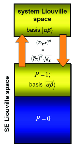
Figure 1: (Color online) Decomposition of the total $SE$ Liouville space into the eigenspaces of the projection operator $\overline{P}$, induced by the uniform statistical operator $\overline{\rho}_{E}$. The unit eigenspace is equivalent to the system Liouville space, where the equivalence is given by the isomorphism (3). Working within the eigenspaces of $\overline{P}$ removes the need for performing the partial trace over the environmental states.

Decomposition of the $SE$ Liouville space into the two eigenspaces of $\overline{P}$ (depicted in Fig. 1) is the essence of the PTF approach: every vector $\mu$ from the $SE$ Liouville space can be written as a column $\mu=[\mu_{1}\;\mu_{2}]^{\mathrm{T}}$, where $\mu_{1}$ belongs to the unit eigenspace of $\overline{P}$ and represents (up to a multiplicative constant $\sqrt{d_{E}}$) the system’s reduced component of $\mu$, i.e., $\mu_{S}\equiv\mathrm{Tr}_{E}\mu=\sqrt{d_{E}}\mu_{1}$. The other component, $\mu_{2}$, belongs to subspace 2 (the zero-eigenspace of $\overline{P}$), where the correlations between $S$ and $E$ reside. It is important to note that the elements of subspace 2 (blue subspace in Fig. 1) have zero trace over environmental states.

In a similar fashion, an operator $A$ acting on the $SE$ Liouville space has a block-form with submatrices $A_{pq}$, $p,q=1,2$, where $A_{11}$ would be the system’s reduced component of this operator. For instance, the block form of the $SE$ Liouvillian $L$ is given by

$$\mathcal{L}=\left[\begin{array}[]{cc}{\mathcal{L}}_{11}&{\mathcal{L}}_{12}\\ {\mathcal{L}}_{21}&{\mathcal{L}}_{22}\end{array}\right],$$ (5)

where ${\mathcal{L}}_{11}$ is commutator-generated, and corresponds to an effective system Hamiltonian ${\mathcal{H}}_{S}+\mathrm{Tr}_{E}({{\mathcal{H}}}_{\mathrm{int}})/d_{E}$. Off-diagonal, non-square Liouvillian submatrices, ${\mathcal{L}}_{12}$ and ${\mathcal{L}}_{21}={\mathcal{L}}_{12}^{\dagger}$, represent the $S$–$E$ interaction as seen in the composite Liouville space – when ${\mathcal{H}}_{\mathrm{int}}$ vanishes, so do ${\mathcal{L}}_{12}$ and ${\mathcal{L}}_{21}$. ${\mathcal{L}}_{22}$ can be perceived as governing the evolution of entangled $SE$ states, and tends to a form fixed by ${{\mathcal{H}}}_{S}$ and ${\mathcal{H}}_{E}$ when the interaction is turned off.

II.2 Equations with memory dressing

Using the notation introduced above, the evolution of the reduced statistical operator $\rho_{S}$ can be represented by

$$\rho_{S}(t)=\mathcal{U}_{11}(t,0)\rho_{S}(0)+\sqrt{d_{E}}\,\mathcal{U}_{12}(t,0)\rho_{2}(0),$$ (6)

where $\mathcal{U}_{11}$ and $\mathcal{U}_{12}$ are the submatrices od the $SE$ evolution operator $\mathcal{U}$, given by

$$\mathcal{U}(t,0) = \mathrm{T^{c}}\exp\left(-i\int_{0}^{t}\left[\begin{array}[]{cc}{\mathcal{L}}_{11}&{\mathcal{L}}_{12}\\ {\mathcal{L}}_{21}&{\mathcal{L}}_{22}\end{array}\right]\,dt\right)$$ (9)

$$= \left[\begin{array}[]{cc}\mathcal{U}_{11}(t,0)&\mathcal{U}_{12}(t,0)\\ \mathcal{U}_{21}(t,0)&\mathcal{U}_{22}(t,0)\end{array}\right].$$ (12)

In Ref. Knezevic and Ferry, 2004, equations of motion for $\mathcal{U}_{11}$ and $\mathcal{U}_{12}$ were derived as

$$\frac{d{\mathcal{U}}_{11}}{dt} = -i\left({\mathcal{L}}_{11}-{\mathcal{L}}_{12}\mathcal{R}\right)\mathcal{U}_{11},\hfill$$ (13a)

$$\frac{d{\mathcal{U}}_{12}}{dt} = -i\left({\mathcal{L}}_{11}-{\mathcal{L}}_{12}\mathcal{R}\right)\mathcal{U}_{12}-i{\mathcal{L}}_{12}\mathcal{V},\hfill$$ (13b)

accompanied by the initial conditions $\mathcal{U}_{11}(0,0)=1$ and $\mathcal{U}_{12}(0,0)=0$. Quantity $\mathcal{R}$ is the so-called memory dressing, as it appears to ”dress” the real physical interaction ${\mathcal{L}}_{12}$ and yield an effective (generally complex) interaction term, $-{\mathcal{L}}_{12}\mathcal{R}$, that accompanies the hermitian term ${\mathcal{L}}_{11}$, responsible for unitary evolution. Memory dressing describes the cumulative effect of the $S-E$ interaction, as witnessed by a quadratic feedback term in its self-contained matrix Riccati Reid (1972); Bittanti et al. (1991) equation of motion (below). The other new quantity occurring in (13), $\mathcal{V}(t,0)$, can be perceived as the evolution operator for the states from subspace 2, and is important for the description of the influx of information from $E$ to $S$. $\mathcal{R}$ and $\mathcal{V}$ obey

$$\frac{d\mathcal{R}}{dt} = -i{\mathcal{L}}_{22}\mathcal{R}-i\mathcal{R}{\mathcal{L}}_{12}\mathcal{R}+i\mathcal{R}{\mathcal{L}}_{11}+i{\mathcal{L}}_{21},\hfill$$ (14a)

$$\frac{d\mathcal{V}}{dt} = -i\left({\mathcal{L}}_{22}+\mathcal{R}{\mathcal{L}}_{12}\right)\mathcal{V},$$ (14b)

accompanied by $\mathcal{R}(0)=0$ and $\mathcal{V}(0,0)=1$.

Equations (13) and (14) are exact:Knezevic and Ferry (2004) they are an alternative form of the $SE$ Liouville equation (1). The resulting exact evolution of the reduced statistical operator can be expressed through the following differential equation of motion

$$\frac{d\rho_{S}(t)}{dt}= - i\left[{\mathcal{L}}_{11}-{\mathcal{L}}_{12}\mathcal{R}(t)\right]\rho_{S}(t)$$ (15)

$$- i{\mathcal{L}}_{12}\sqrt{d_{E}}\mathcal{V}(t,0)\mathcal{\rho}_{2}(0).$$

which is a partial-trace-free form of $\frac{d\rho_{S}}{dt}=\mathrm{Tr}_{E}(-iL\rho)$.

If we restrict our attention to the evolution starting from an initially uncorrelated state of the form

$$\rho(0)=\rho_{E}(0)\otimes\rho_{S}(0),$$ (16)

it is possible to completely reduce the problem to subspace $1$. Namely, it is possible to write

$$\rho_{2}(0)=\mathcal{M}\rho_{1}(0)=d_{E}^{-1/2}\mathcal{M}\rho_{S}(0),$$ (17)

where the mapping $\mathcal{M}$ is completely determined by the components of $\rho_{E}(0)$, the initial environment statistical operator (see Appendix A). Equation (17) embodies the argument made by Lindblad Lindblad (1996) that a subdynamics exists only for an uncorrelated initial state, because, as a consequence of (6) and (17), it is possible to write

$$\rho_{S}(t)=\underbrace{[\mathcal{U}_{11}(t,0)+\mathcal{U}_{12}(t,0)\mathcal{M}]}_{\mathcal{W}(t,0)}\rho_{S}(0),$$ (18)

so the evolution is completely described on the Liouville space of the open system. When (17) is substituted into (15), we obtain the differential form of (18) as

$$\frac{d\rho_{S}(t)}{dt}=-i\left[{\mathcal{L}}_{11}-{\mathcal{L}}_{12}\mathcal{R}(t)\right]\rho_{S}(t)-i{\mathcal{L}}_{12}\mathcal{V}(t)\mathcal{M}\rho_{S}(0).$$ (19)

It is well known that a subdynamics can also be obtained for the case of an initially decoupled $SE$ state by simply choosing the initial environmental statistical operator $\rho_{E}$ as the one to induce the projection operator $P$ (see, for instance, Ref. Breuer and Petruccione, 2002). However, the result for the final dynamics must not depend on the projection operator used, as projection operators are, after all, only auxiliary quantities. While the physics must be the same regardless of the projection operator used, the opacity of the equations obtained certainly varies. Equation (19) shows explicitly how the subdynamics looks for $\overline{P}$; by generalizing the proof in Appendix A, one can write the subdynamics for any other projection operator instead of $\overline{P}$. The reason we are using $\overline{P}$ instead of the projection operator $P$ induced by the initial environmental statistical operator is that, as stated previously, $\overline{P}$ is the only projection operator that has an orthonormal eigenbasis in which it is represented by a diagonal form (4). While any other projection operator $P$ still projects onto its own $d_{S}^{2}$-dimensional image space (see Appendix A), $P$ and $1-P$ never assume simple diagonal forms, so after projecting one still needs to explicitly take the partial trace, which leaves the equations less transparent.

III Decoherence in the presence of a ”memoryless” environment

The non-Markovian map $\mathcal{W}(t,0)=\mathcal{U}_{11}(t,0)+\mathcal{U}_{12}(t,0)\mathcal{M}$ that defines the subdynamics (18) can quite generally be written as

$$\mathcal{W}(t,0)=\mathrm{T^{c}}\exp{\left(\int_{0}^{t}\mathcal{K}(t^{\prime})\,dt^{\prime}\right)}.$$ (20)

Here, $\mathcal{K}(t)$ is the generator of $\mathcal{W}(t,0)$. In general, $\mathcal{K}(t)=-i\mathcal{L}_{\mathrm{eff}}-\mathcal{G}(t)$, i.e., it contains an effective system Liouvillian $\mathcal{L}_{\mathrm{eff}}$ and a correction $\mathcal{G}$ due to the system-environment interaction, which describes decoherence. In case of Markovian evolution, $\mathcal{K}=-i\mathcal{L}_{\mathrm{eff}}-\mathcal{G}=\mathrm{const.}$, and $\mathcal{G}$ must have the well-known Lindblad dissipator form Lindblad (1976); Alicki and Lendi (1987) in order for the map (20) to remain completely positive. Alicki and Lendi (1987); Breuer and Petruccione (2002)

In general, it is impossible to obtain $\mathcal{W}(t,0)$ exactly. If one is interested in retaining the non-Markovian nature of (20), typically an expansion up to the second or fourth order in the interaction is undertaken. Breuer and Petruccione (2002) On the other hand, a Markovian approximation to the exact dynamics can be obtained in the weak-coupling and van Hove limit, as first shown by Davies. Davies (1974) Although the weak coupling limit has been used previously by several authors Li et al. (2005); Pedersen and Wacker (2005) to derive Markovian rate equations for tunneling structures in the resonant-level model, this approximation is not generally applicable for nanostructures. Li et al. (2005)

The point we wish to make here is that the Markovian approximation to the long-time evolution of nanostructures can be justified more broadly, by employing the approximation of a memoryless environment for the contacts. Consider first the active region of a small semiconductor device; a good example is the state-of-the art MOSFET with 45 nm lithographic gate length (physical gate length is estimated to be around 20 nm), found in Intel’s 2008 Penryn processors. Int Semiconductor devices are generally required to operate at (or at least near) room temperature, where phonons are abundant. However, due to the active region’s minuscule dimensions, scattering happens infrequently, so the active region does feature quasiballistic transport, where scattering can be added as a perturbation to the ballistic solution. The bulk-like contacts of semiconductor devices are typically heavily doped (e.g., $\sim 10^{19}-10^{20}\;\mathrm{cm}^{-3}$ in silicon), and at room temperature all the dopants are ionized; at such high doping densities, electron-electron scattering dominates over phonon scattering as the leading energy-relaxation mechanism (e.g., relaxation time for electron-electron scattering in bulk GaAs at $10^{19}\;\mathrm{cm}^{-3}$ and room temperature is $10$ fs, Kriman et al. (1990) whereas it is about $150$ fs for polar optical phonon scattering Lundstrom (2000)). Basically, electron-electron scattering in the highly doped contacts of semiconductor devices ensures that the carrier distribution snaps into a distribution that can be considered a displaced (also known as drifted) Fermi-Dirac distribution Lugli and Ferry (1985) (see also Sec. IV.1) within the energy-relaxation time $\tau\approx 10^{1}-10^{2}$ femtoseconds Osman and Ferry (1987); Kriman et al. (1990) (the actual value depends on the doping density and temperature). This time is very short with respect to the typical response times of these devices, which is on the timescales of $\tau_{AR}\approx 1-10$ ps (”AR” stands for the active region). Therefore, for small semiconductor devices, on timescales coarsened over the energy relaxation time $\tau$ of the contacts, the contact distribution function responds virtually instantaneously, and the contacts can be considered memoryless, while the relaxation of the whole structure happens on timescales a few orders of magnitude longer. (A memoryless approximation must be applied with care to current-carrying contacts, as we will discuss in detail in IV.1 and IV.3.)

For low-dimensional nanostructures, fabricated on a high-mobility two-dimensional electron gas (2DEG) and operating at low temperatures, the energy relaxation in the contacts is also governed by the inelastic electron-electron scattering, Altshuler and Aronov (1979, 1981) because the phonons are frozen (although there are indications that acoustic phonon scattering may be important down to about 4 K Lutz et al. (1993)). The near-equilibrium energy relaxation times in these contacts are much longer than in devices, falling in the wide range of $10^{0}-10^{3}$ ps, Giuliani and Quinn (1982); Fasol (1991); Noguchi et al. (1996); Kabir et al. (2006) depending on the contact dimensionality (1DAltshuler et al. (1982); Wind et al. (1986); Linke et al. (1997); Le Hur (2006) or 2D Giuliani and Quinn (1982); Fasol (1991)), carrier density, and temperature. Excitations with energies higher than $k_{B}T$, such as when bias $V>k_{B}T/q$ is applied across the nanostructure ($q$ is the electron charge), relax more rapidly, Fasol (1991); Linke et al. (1997) which is of particular importance in the collector contact. In low-dimensional nanostructures, there are also experimental indications that coupling of the active region to the contacts governs its evolution. Pivin et al. (1999) As for the typical response times of nanostructures, recent experiment by Naser et al. Naser et al. (2006) demonstrated Markovian relaxation in quantum point contacts on $\tau_{AR}\approx 50$ ns timescales at 4 K, so the ratio $\tau/\tau_{AR}$ is still less than unity, but not as small as in devices.

Still, there is enough rationale to further explore a nanostructure’s dynamics within the approximation of memoryless contacts, with the understanding that this approximation must generally be qualified, especially for nanostructures at very low temperatures. We will therefore proceed with deriving the Markovian approximation to the exact non-Markovian equation (19) in the presence of an environment that loses memory on a timescale $\tau$, presumed much shorter that the response time of the open system, and we will derive the relationships that the coarse graining time $\tau$ must satisfy for the approximation to be consistent. Then, in Sec. IV, we will see what type of constraint that puts on our energy relaxation time in the contacts.

Before proceeding with the formal development, it is worth stressing that the importance of a Markovian approximation to the exact evolution is great, because with both nanoscale semiconductor devices used for digital applications and with DC experiments on nanostructures, one is primarily interested in the steady state that the structure reaches upon the application of a DC bias. In these situations, it is sufficient to employ the Markovian approximation to the evolution (if warranted), as it is correct on long timescales and will result in the correct steady state.

III.1 Markovian evolution by coarse graining

To practically obtain the Markovian approximation due to an environment that loses memory after a time $\tau$, we use the coarse-graining procedure: we can partition the time axis into intervals of length $\tau$, $t_{n}=n\tau$, so the environment interacts with the system in exactly the same way during each interval $[t_{n},t_{n+1}]$, Lidar et al. (2001) so

$$\frac{\rho_{S,n+1}-\rho_{S,n}}{\tau}=\mathcal{\overline{K}}_{\tau}\rho_{S,n},$$ (21)

where $\mathcal{\overline{K}}_{\tau}=\frac{\int_{0}^{\tau}\mathcal{K}(t^{\prime})dt^{\prime}}{\tau}=\frac{\int_{t_{n}}^{t_{n+1}}\mathcal{K}(t^{\prime})dt^{\prime}}{\tau}$ is the averaged value of the map’s generator over any interval $[t_{n},t_{n+1}]$ ($\mathcal{K}$ is reset at each $t_{n}$). If the timescales are coarsened over $\tau$, then the term on the left of (21) approximates the first derivative at $t_{n}$, so the system’s evolution can be described by

$$\frac{d\rho_{S}}{dt}=\mathcal{\overline{K}}_{\tau}\rho_{S}(t).$$ (22)

The above map is completely positive and Markovian (coarse graining preserves complete positivity Lidar et al. (2001)), but still has little practical value, because extracting $\mathcal{K}$ explicitly from first principles is difficult. However, if the coarse-graining time $\tau$ is short enough, then the short-time expansion of $\mathcal{K}$ can be used to perform the coarse-graining. Up to the second order in time (details of the short-time expansion can be found in Appendix B),

$$\mathcal{K}(t)=-i\mathcal{L}_{\mathrm{eff}}-2\Lambda t+o(t^{2}),$$ (23)

where ${\mathcal{L}}_{\mathrm{eff}}=[{\mathcal{H}}_{S}+\langle{{\mathcal{H}}_{\mathrm{{int}}}}\rangle,\dots]=\mathcal{L}_{S}+[\langle{{\mathcal{H}}_{\mathrm{{int}}}}\rangle,\dots]$ is an effective system Liouvillian, containing the noninteracting-system Liouvillian $\mathcal{L}_{S}$ and a correction due to the interaction [$\langle\dots\rangle=\mathrm{Tr}_{E}[\rho_{E}(0)\dots]$ denotes the partial average with respect to the initial environmental state $\rho_{E}(0)$]. The matrix elements of superoperator $\Lambda$, in a basis $\alpha\beta$ in the system’s Liouville space (Liouville space is basically a tensor square of the Hilbert space), are determined from the matrix elements of the interaction Hamiltonian:

$${\Lambda}^{\alpha\beta}_{\alpha^{\prime}\beta^{\prime}}=\frac{1}{2}\left\{\left\langle{{\mathcal{H}}}_{\mathrm{int}}^{2}\right\rangle^{\alpha}_{\alpha^{\prime}}\delta^{\beta^{\prime}}_{\beta}+\left\langle{{\mathcal{H}}}_{\mathrm{int}}^{2}\right\rangle^{\beta^{\prime}}_{\beta^{\prime}}\delta^{\alpha}_{\alpha^{\prime}}\right.\quad\hfill$$

$$-2\sum_{j,j^{\prime}}\left({{\mathcal{H}}}_{\mathrm{int}}\right)^{j^{\prime}\alpha}_{j\alpha^{\prime}}\rho_{E}^{j}\left({{\mathcal{H}}}_{\mathrm{int}}\right)^{j\beta^{\prime}}_{j^{\prime}\beta}\quad\quad\hfill$$ (24)

$$-\left.\left(\langle{\mathcal{H}}_{\mathrm{int}}\rangle^{2}\right)^{\alpha}_{\alpha^{\prime}}\delta^{\beta^{\prime}}_{\beta}+2\langle{\mathcal{H}}_{\mathrm{int}}\rangle^{\alpha}_{\alpha^{\prime}}\langle{\mathcal{H}}_{\mathrm{int}}\rangle^{\beta^{\prime}}_{\beta}-\left(\langle{\mathcal{H}}_{\mathrm{int}}\rangle^{2}\right)^{\beta^{\prime}}_{\beta}\delta^{\alpha}_{\alpha^{\prime}}\right\},$$

where $\rho_{E}^{j}$ are the eigenvalues of the initial environment statistical operator $\rho_{E}(0)$. $\Lambda$ has implicitly been defined previously Alicki (1989) in the interaction picture and with the assumption of $\langle{\mathcal{H}}_{\mathrm{int}}\rangle=0$. Here, we work in the Schrödinger picture and generally need to retain $\langle{\mathcal{H}}_{\mathrm{int}}\rangle\neq 0$, which is important for the inclusion of carrier-carrier interaction in nanostructures. ${\Lambda}$ contains essential information on the directions of coherence loss.

If the coarse-graining time $\tau$ is short enough that it holds

$$\left\|\Lambda\right\|\tau\ll\left\|\mathcal{L}_{\mathrm{eff}}\right\|,$$ (25)

then the short-time expansion of $\mathcal{K}$ can be used for coarse-graining, and we obtain

$$\mathcal{\overline{K}}_{\tau}=-i\mathcal{L}_{\mathrm{eff}}-\Lambda\tau,$$ (26)

leading to the Markovian equation

$$\frac{d\rho_{S}(t)}{dt}=\left(-i\mathcal{L}_{\mathrm{eff}}-\Lambda\tau\right)\rho_{S}(t),$$ (27)

which is the central equation of this paper. For the Markovian approximation to be consistent, Breuer and Petruccione (2002) the system’s relaxation (occurring on timescales no shorter than $1/\|\Lambda\|\tau$) must be much slower than the environment’s relaxation (occurring over $\tau$), therefore we must have

$$\left\|\Lambda\right\|{\tau}^{2}\ll 1.$$ (28)

Conditions (25) and (28) can compactly be written as

$$\left\|\Lambda\right\|{\tau}^{2}\ll\min{\{1,\left\|\mathcal{L}_{\mathrm{eff}}\right\|\tau\}}.$$ (29)

III.2 Some general considerations regarding the use of Eq. (27)

Before we proceed to treating a concrete nanostructure as an example, there are several general features regarding the use of Eq. (27) that can be used more broadly than in the treatment of nanostructures. (The reader interested exclusively in decoherence in nanostructures can skip the rest of this section and go directly to Sec. IV.)

III.2.1 Decoherence-free evolution in the zero-eigenspace of ${\Lambda}$

Let us assume for a moment that $\mathcal{L}_{\mathrm{eff}}$ and ${\Lambda}$ commute (we will see two cases of this situation in Appendix C). If so, the components of $\rho_{S}$ belonging to the null-space of ${\Lambda}$ will not decohere – they will continue to evolve unitarily, as the null-space of ${\Lambda}$ will be invariant under $\mathcal{L}_{\mathrm{eff}}$. Components of $\rho_{S}$ corresponding to the nonzero eigenvalues of ${\Lambda}$ will decohere until they drop to zero. So in the case of commuting $\mathcal{L}_{\mathrm{eff}}$ and ${\Lambda}$, null-space of ${\Lambda}$ is decoherence-free. For non-commuting $\mathcal{L}_{\mathrm{eff}}$ and ${\Lambda}$, this statement can be generalized to

Theorem 1. If a subspace of $\mathcal{N}({\Lambda})$, the null-space of operator ${\Lambda}$, is also an invariant subspace of $\mathcal{L}_{\mathrm{eff}}$, then it supports decoherence-free (unitary) evolution according to the map (27).

Proof. Let $\mathcal{N}^{\prime}({\Lambda})$ be a subspace of $\mathcal{N}({\Lambda})$. If $\mathcal{N}^{\prime}({\Lambda})$ is an invariant subspace of $\mathcal{L}_{\mathrm{eff}}$, then it is an invariant subspace of the full generator of the Markovian semigroup (27), and consequently an invariant subspace of the semigroup. A statistical operator $\rho^{0}$, initially prepared in $\mathcal{N}^{\prime}({\Lambda})$, would remain in $\mathcal{N}^{\prime}({\Lambda})$ at all times, and evolve unitarily according to $\frac{d\rho^{0}}{dt}=-i\mathcal{L}_{\mathrm{eff}}^{0}\rho^{0}(t)$, where $\mathcal{L}_{\mathrm{eff}}^{0}$ is the reduced form of $\mathcal{L}_{\mathrm{eff}}$ onto $\mathcal{N}^{\prime}({\Lambda})$. $\blacksquare$

This theorem is equivalent to the statements made in the original works on decoherence-free subspaces Lidar et al. (1998), where a decoherence-free statistical operator was defined through annulment by the Lindblad dissipator. Note, however, that here we identify the decoherence-free subspaces in the system Liouville space, rather than in its Hilbert space. This allows for the possibility that some entangled system states ($\mathrm{Tr}\rho_{S}^{2}\neq\mathrm{Tr}\rho_{S}$) could be resilient against decoherence, which is a potentially useful feature that cannot be captured in the Hilbert space alone.

Theorem 1 gives us a straightforward, general recipe for the classification of the decoherence-free subspaces in the case of Markovian dynamics (27). What one needs to do is to construct the operator ${\Lambda}$ according to Eq. (III.1), from the microscopic interaction Hamiltonian and the environmental preparation, solve its eigenproblem (in general numerically), and investigate whether any of its null-spaces is invariant under $\mathcal{L}_{\mathrm{eff}}.$ This is a simple, efficient way to approximately determine where the information should be stored, and should work well as long as the system is small enough to allow for a full solution to the eigenproblem of $\Lambda$.

Moreover, the structure of the eigenspaces of ${\Lambda}$ enables us to determine the directions of decoherence. For instance, regardless of the value of $\tau$, we can still tell which states do and which do not decohere, and calculate the relative values of the decoherence rates for two given states. For fast switching in nanoscale semiconductor devices, for example, we need rapid coherence loss between the active region and leads, and we may therefore opt to prepare the system in the subspace of $\Lambda$ corresponding to one of its largest eigenvalues.

III.2.2 Identification of the steady state

An important special case of a decoherence-free subspace is that of a vector belonging to the intersection of $\mathcal{N}(\mathcal{L}_{\mathrm{eff}})$ and $\mathcal{N}(\Lambda)$.

Theorem 2. A statistical operator belonging to $\mathcal{N}({\mathcal{L}_{\mathrm{eff}}})\cap\mathcal{N}({\Lambda})$, the intersection of the null-spaces $\mathcal{N}(\mathcal{L}_{\mathrm{eff}})$ and $\mathcal{N}(\Lambda)$, is a steady state for the evolution according to the map (27).

Proof. $\mathcal{N}({\mathcal{L}_{\mathrm{eff}}})\cap\mathcal{N}({\Lambda})$ is the null space of the Markovian semigroup generator. Consequently, any statistical operator prepared in $\mathcal{N}({\mathcal{L}_{\mathrm{eff}}})\cap\mathcal{N}({\Lambda})$ remains unchanged at all times, satisfying the definition of a steady state. $\blacksquare$

By looking into the common null-subspace of both $\mathcal{L}_{\mathrm{eff}}$ and $\Lambda$, one can narrow down the set of potential steady states, which is important in many-body transport calculations. In the case of a many-particle open system, a full solution to the eigenproblem of $\Lambda$ may not be tractable; however, identification of the common null-space of $\mathcal{L}_{\mathrm{eff}}$ and $\Lambda$ may be.

III.2.3 A comment on the validity of Eq. (27)

In general, whenever an efficient resetting mechanism can be defined for the environment, so that Eq. (29) is satisfied, (27) should be applicable. However, it also appears that the simple equation (27) may be used more broadly than specified by (29). Namely, on one of the few exactly solvable systems, the spin boson model with pure dephasing, which experiences Markovian evolution in the long time limit regardless of the coupling strength, it can be shown (see Appendix C.1) that one can define a mathematical coarse graining time $\tau$ that is shorter than any other timescale in the coupled system and environment, so that coarse-grained evolution over $\tau$ (27) and the exact Markovian evolution coincide. So, it appears that not only does coarse graining result in Markovian maps, but the converse might also be true: it is possible that a given Markovian evolution can be obtained by coarse graining of the short-time dynamics if a suitable (ultrashort) mathematical coarse graining time is chosen. This statement would, of course, be very difficult to prove in general terms, but is interesting because it would mean that all one needs to deduce the steady state for the evolution of an open system is the information on its short-time dynamics (23), which can in principle be done relatively straightforwardly and from first principles (the microscopic interaction and the preparation of the environment). Indeed, on an additional example of the Jaynes-Cummings Hamiltonian in the rotating wave approximation, which has been worked out in Appendix C.2, it has been shown that by using map (27) and the resulting criterion for the steady state (Theorem 2), relaxation towards the proper equilibrium state has been obtained. So it appears that the applicability of Eq. (27) may extend beyond the formal range of its validity (29).

IV A Two-Terminal Ballistic Nanostructure

In this Section, we consider a generic two-terminal nanostructure under bias, and introduce a model interaction between the ballistic active region and the contacts. This model should hold regardless of whether the structure has resonances or not, as it is constructed to mimic the source term in the single-particle density matrix Jacoboni (1992); Rossi and Jacoboni (1992); Brunetti et al. (1989); Hohenester and Pötz (1997); Ciancio et al. (2004); Platero and Aguado (2004) and Wigner function Kluksdahl et al. (1989); Pötz (1989); Frensley (1990); Bordone et al. (1999); Biegel and Plummer (1997); Jensen and Buot (1989); Grubin and Buggeln (2002); Shifren et al. (2003); Jacoboni et al. (2003); Nedjalkov et al. (2004, 2006) formalisms, and preserve the continuity of current, state-by-state. In Sec. IV.4, the results are illustrated on a one-dimensional two-barrier tunneling structure.

The left contact is the injector (source), biased negatively, while the right contact is the collector (drain). The contact-active region boundaries are at $x_{L}$ (left) and $x_{R}$ (right), with $W=x_{R}-x_{L}$ being the active region width. We will assume that the active region includes a large enough portion of the contacts (i.e., exceeding several Debye lengths) so that there is no doubt about the flat-band condition in the contacts. Also, $W$ should be large enough to reasonably ensure a quasicontinuum of wavevectors ($\Delta k=2\pi/W$) following the periodic boundary conditions. While sweeping the negative bias on the injector contact, we will assume that it is done slowly (so that between two bias points the system is allowed to relax) and in small increments (so that the potential profile inside the active region does not change much between two bias points, and can be regarded constant during each transient).

For every energy $\mathcal{E}_{k}$ above the bottom of the left contact, the active region’s single particle Hamiltonian has two eigenfunctions, a forward ($\Psi_{k}$) and a backward ($\Psi_{-k}$) propagating state, that can be found by (in general numerically) solving the single-particle Schrödinger equation for a given potential profile in the active region. To keep the discussion as general as possible, we will not specify the details of how the active region actually looks (Fig. 2) – e.g., it can be a heterostructure, a pn homojunction, or a MOSFET channel – but we will require that the contact-active region open boundaries (at $x_{L}$ and $x_{R}$) are far enough from any junctions in the active region, so that the behavior of $\Psi_{\pm k}$ near the junctions is already plane-wave like, i.e., that their general form near the injector is $\Psi_{k}(x_{L}^{+})=e^{ik{x_{L}^{+}}}+r_{-k,L}e^{-ik{x_{L}^{+}}},\;\Psi_{-k}({x_{L}^{+}})=t_{-k,L}e^{-ik{x_{L}^{+}}},$ while near the collector $\Psi_{k}({x_{R}^{-}})=t_{k^{\prime},R}e^{ik^{\prime}{x_{R}^{-}}},\;\Psi_{-k}({x_{R}^{-}})=e^{-ik^{\prime}{x_{R}^{-}}}+r_{k^{\prime},R}e^{ik^{\prime}{x_{R}^{-}}}$. Here, where $t$’s and $r$’s are the transmission and reflection amplitudes, while $k$ and $k^{\prime}$ are the wavevectors that correspond to the same energy $\mathcal{E}_{k}$, measured with respect to the conduction band bottoms in the left and right contacts, respectively ($k^{2}=k^{\prime 2}-2mqV/\hbar^{2}=2m\mathcal{E}_{k}/\hbar^{2}$, where $-V$ has been applied to the left contact, and $q$ is the electron charge).

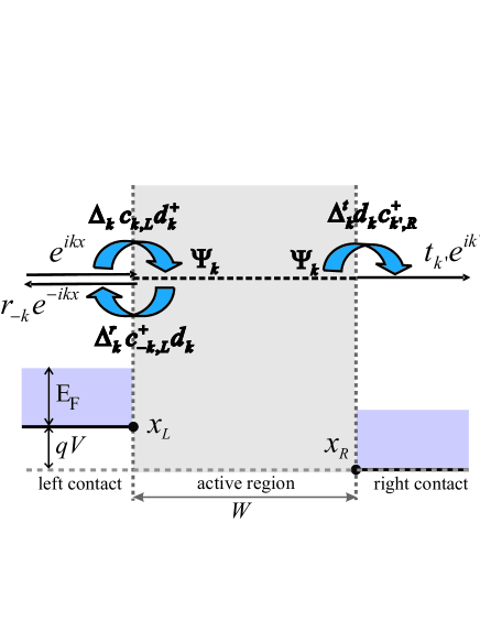
Figure 2: (Color online) Schematic of the coupling between the active region of a generic two-terminal nanostructure and the contacts. In case of ballistic injection through the open boundaries, a forward-propagating state $\Psi_{k}$ is coupled with the states $\exp(\pm ikx)$ in the left contact (injected and reflected wave) and the state $\exp(ik^{\prime}x)$ in the right contact (transmitted wave) via a hopping model interaction (IV).

Associated with $\Psi_{k}$ ($\Psi_{-k}$) in the active region are the creation and destruction operators $d_{k}^{\dagger}$ and $d_{k}$ ($d_{-k}^{\dagger}$ and $d_{-k}$), so the active region many-body Hamiltonian is

$$\mathcal{H}_{S}=\sum_{k>0}\mathcal{\omega}_{k}(d_{k}^{\dagger}d_{k}+d_{-k}^{\dagger}d_{-k}).$$ (30)

Spin is disregarded, and $\omega_{k}=\mathcal{E}_{k}/\hbar$. In case of ballistic injection through the open boundaries, each state $\Psi_{k}$ is naturally coupled with the states $\exp(\pm ikx)$ in the left contact (injected and reflected wave) and the state $\exp(ik^{\prime}x)$ in the right contact (transmitted wave). For $\Psi_{-k}$, the coupling is between $\exp(\pm ik^{\prime}x)$ in the right and $\exp(-ikx)$ in the left contact. To model this coupling via a hopping-type interaction, we can write quite generally (see Fig. 2)

$$\mathcal{H}_{\mathrm{int}}^{+} = \sum_{k>0}\left(\Delta_{k}d_{k}^{\dagger}c_{k,L}+\Delta_{k}^{r}c_{-k,L}^{\dagger}d_{k}+\Delta_{k}^{t}c_{k^{\prime},R}^{\dagger}d_{k}\right)+h.c.$$

$c^{\dagger}_{\pm k,L}$ ($c_{\pm k,L}$) and $c^{\dagger}_{k^{\prime},R}$ ($c_{k^{\prime},R}$) create (destroy) an electron with a wavevector $\pm k$ in the left and $k^{\prime}$ in the right contact, respectively. The hopping coefficients $\Delta_{k}$, $\Delta_{k}^{r}$ and $\Delta_{k}^{t}$ are the rates of injection, reflection, and transmission, respectively. Therefore, they are proportional to the injected, reflected, and transmitted current for the state $\Psi_{k}$, i.e.,

$$\frac{\Delta_{k}^{r}}{\Delta_{k}}=\mathcal{R}_{k},\;\;\frac{\Delta_{k}^{t}}{\Delta_{k}}=\mathcal{T}_{k},$$ (32)

where $\mathcal{R}_{k}$ and $\mathcal{T}_{k}$ are the reflection and transmission coefficient at a given energy. The actual magnitude of $\Delta_{k}$ can be determined by requiring that $\Delta^{t}_{k}=\mathcal{T}_{k}\Delta_{k}$, the hopping rate from the active region into the right contact, be the same as the current (per unit charge) carried through the active region by $\Psi_{k}$. This just means there is no more reflection once the wave exits the active region and gets into the outgoing contact, and is usually referred to as the assumption of reflectionless leads. Datta (1995)) The current carried by $\Psi_{k}$ is given by the well-known quantum-mechanical relationship

$$I_{k} = \frac{q\hbar}{m\|\Psi_{k}\|^{2}}\mathrm{Im}\left(\Psi_{k}^{*}\nabla\Psi_{k}\right)$$ (33)

$$= \frac{q\hbar}{m}\frac{|t_{k^{\prime},R}|^{2}k^{\prime}}{\left\|\Psi_{k}\right\|^{2}}=\frac{q\hbar k}{m}\frac{\mathcal{T}_{k}}{\left\|\Psi_{k}\right\|^{2}},$$

where we have used the form of $\Psi_{k}$ near the right contact $t_{k^{\prime},R}e^{ik^{\prime}x}$, and ${\left\|\Psi_{k}\right\|^{2}}=\int_{0}^{W}dx|\Psi_{k}(x)|^{2}$ is the norm squared of $\Psi_{k}$ over the active region of width $W$. Since we require that $I_{k}/q=\Delta^{t}_{k}=\mathcal{T}_{k}\Delta_{k}$, we find

$$\Delta_{k}=\frac{\hbar k}{m\left\|\Psi_{k}\right\|^{2}}.$$ (34)

Finally,

$$\mathcal{H}_{\mathrm{int}}^{+} = \sum_{k>0}\Delta_{k}\left(d_{k}^{\dagger}c_{k,L}+\mathcal{R}_{k}c_{-k,L}^{\dagger}d_{k}+\mathcal{T}_{k}c_{k^{\prime},R}^{\dagger}d_{k}\right)+h.c.,$$

while the Hamiltonian for the backward propagating states can be written in an analogous fashion, as

$$\mathcal{H}_{\mathrm{int}}^{\mathrm{-}} = \sum_{k>0}\Delta_{-k}\left(d_{k}^{\dagger}c_{-k^{\prime},R}+\mathcal{R}_{-k}c_{k^{\prime},R}^{\dagger}d_{k}+\mathcal{T}_{-k}c_{k^{\prime},R}^{\dagger}d_{k}\right)+h.c.$$

with $\Delta_{-k}=\frac{\hbar k^{\prime}}{m\|\Psi_{-k}\|^{2}}$, and $\mathcal{T}_{k}=\mathcal{T}_{-k}$, $\mathcal{R}_{k}=\mathcal{R}_{-k}$.

When we put it all together, we have for the interaction Hamiltonian of the active region with the left/right contact:

$$\mathcal{H}_{\mathrm{int}}^{L} = \sum_{k>0}\Delta_{k}\left\{\left(c_{k,L}^{\dagger}+\mathcal{R}_{k}c_{-k,L}^{\dagger}\right)d_{k}\right.$$

$$+ \left.d_{k}^{\dagger}\left(c_{k,L}+\mathcal{R}_{k}c_{-k,L}\right)\right\}$$

$$+ \Delta_{-k}\left\{\mathcal{T}_{k}c_{-k,L}^{\dagger}d_{-k}+\mathcal{T}_{k}d_{-k}^{\dagger}c_{-k,L}\right\},$$

$$\mathcal{H}_{\mathrm{int}}^{R} = \sum_{k>0}\Delta_{-k}\left\{\left(c_{-k^{\prime},R}^{\dagger}+\mathcal{R}_{k}c_{k^{\prime},R}^{\dagger}\right)d_{-k}\right.$$

$$+ \left.d_{-k}^{\dagger}\left(c_{-k^{\prime},R}+\mathcal{R}_{k}c_{k^{\prime},R}\right)\right\}$$

$$+ \Delta_{k}\left\{\mathcal{T}_{k}c_{k^{\prime},R}^{\dagger}d_{k}+\mathcal{T}_{k}d_{k}^{\dagger}c_{k^{\prime},R}\right\}.$$

IV.1 Current-Carrying Contacts and the Approximation of a Memoryless Environment

Now that we have the interaction Hamiltonians in place, we should evaluate the matrix elements of the superoperator $\Lambda$, which leads us to the questions how the approximation of a memoryless environment is actually applied to contacts carrying current, and how the expectation values of the interaction Hamiltonian are to be calculated.

In general, as the current flows through the structure, we must allow for different distributions of the forward and backward propagating waves in the left and right contacts to ensure current continuity. A simple and often employed approximation for the steady-state distribution in the contacts carrying current $I$ is a single-parameter drifted (or displaced) Fermi-Dirac distribution Fischetti (1998, 1999)

$${f}^{L}_{\pm k}=\langle n_{\pm k,L}\rangle=\frac{1}{\exp\left\{\frac{\hbar^{2}[(\pm k-k_{d})^{2}-k_{F}^{2}]}{2mk_{B}T}\right\}+1}.$$ (38)

Here, $k_{F}$ is the Fermi wavevector and $k_{d}$ is the drift wavevector, determined from the total current $I$ as $k_{d}=mI/n_{1D}q\hbar$, where $n_{1D}$ is the 1D carrier density in each contact (contacts are assumed identical). A drifted Fermi-Dirac distribution, with the temperature equal to that of the lattice, is often employed when we are interested in just the first two moments of the distribution function (i.e., maintaining charge neutrality and ensuring current continuity). Additionally, if needed, information on the electron heating can be incorporated in this distribution by allowing for a discrepancy between the electronic and lattice temperatures (we will neglect electron heating here). Detailed ensemble Monte Carlo - molecular dynamics simulations of carrier transport in highly doped ($>10^{17}\;\mathrm{cm}^{3}$) bulk semiconductors, in which electron-electron scattering is the most efficient energy relaxation mechanism, have shown to produce distributions very close to the drifted Fermi-Dirac distribution (38), Lugli and Ferry (1985, 1986); Kriman et al. (1990) which is generally accepted as a decent approximation for these systems. Here, we will also adopt (38) for the distribution of carriers in the current-carrying contacts, and it is reasonable if the (one-dimensional) contacts are longer than $\sqrt{D\tau}$, where $D$ is the diffusion constant (otherwise, the distribution function in them may not be thermalized Pothier et al. (1997); Pierre et al. (2001)).

Now, the question arises what happens if we try to sweep the voltage. We have mentioned before that the voltage is to be swept slowly (enough time between two bias points for the system to relax) and in small increments (so that we can consider the barrier as having a constant profile during each transient). The latter is crucial for the implementation of the approximation of a memoryless environment. Suppose that, at a bias $V$, a steady-state current $I$ is flowing through the structure. If we increase the bias to $\Delta V$ at $t=0$, where $\Delta V$ is very small, within the first $t=\tau$, the current is virtually unchanged – it takes the current a much longer time $\tau_{AR}\gg\tau$ to change significantly (AR stands for ”active region”; once we have had a chance to complete the calculation, we will see that $\tau_{AR}$ will be equal to $1/\lambda\tau$, where $\lambda$ is a relevant eigenvalue of $\Lambda$). Therefore, after $\tau$, the contact carriers have redistributed themselves to the old distribution function that they had at $V$. Basically, the contact carriers as redistributing themselves to Eq. (38) determined by the (virtually) instantaneous current level at each $\tau$; the current, however, changes very little during each $\tau$. By the time the current has saturated ($\sim\tau_{AR}$), the contact carriers have had a chance to get redistributed many times; however, if the total voltage increase $\Delta V$ is very small, the total current increase during the full transient will also be small, so we can say that during the whole transient the distribution functions of the forward and backward propagating states have been resetting to nearly the same distribution, approximately the average of $f_{\pm k}^{L,R}$ over the interval $[V,V+\Delta V]$. Clearly, as the voltage sweep increment $\Delta V\rightarrow 0$, we can say that during a transient the contacts redistribute to $f_{\pm k}^{L,R}$ (38) at $V$.

Evaluation of $k_{d}$ that enters the contact distribution functions at a given voltage must be done self-consistently: starting with a guess for $k_{d}$ at a given voltage, steady-state distributions and current are evaluated (as detailed in the next section). The obtained current is then used to recalculate $k_{d}$, and the process is repeated until a satisfactory level of convergence is achieved. (Of course, the initial guess for $k_{d}$ at any voltage can be $k_{d}=0$, but for faster convergence it is better to start with the $k_{d}$ found for the preceding voltage.)

IV.2 Markovian Relaxation for a Two-Terminal Nanostructure. Steady-State Distributions and Current

Since the interaction Hamiltonians (37) are linear in the contact creation and destruction operators, and we can approximate that each contact snaps back to a ”drifted” grand-canonical statistical operator, we have $\langle\mathcal{H}_{\mathrm{int}}^{L/R}\rangle=0$. This means that ${\mathcal{L}}_{S}=\mathcal{L}_{\mathrm{eff}}$, and also leaves us with only the first three terms in Eq. (III.1) for $\Lambda$ to calculate. One can show that $\Lambda=\Lambda^{L}+\Lambda^{R}$, where

$$(\Lambda^{L/R})^{\alpha,\beta}_{\alpha^{\prime},\beta^{\prime}} = \frac{1}{2}\left(\langle\left({\mathcal{H}}_{\mathrm{int}}^{L/R}\right)^{2}\rangle^{\alpha}_{\alpha^{\prime}}\delta^{\beta^{\prime}}_{\beta}+\langle\left({\mathcal{H}}_{\mathrm{int}}^{L/R}\right)^{2}\rangle^{\beta^{\prime}}_{\beta}\delta^{\alpha}_{\alpha^{\prime}}\right)$$ (39)

$$- \sum_{i,j}\rho_{L,R}^{i}({\mathcal{H}}_{\mathrm{int}}^{L/R})^{j\alpha}_{i\alpha^{\prime}}({\mathcal{H}}_{\mathrm{int}}^{L/R})^{i\beta^{\prime}}_{j\beta}.$$

The first and the second term in Equation (39) give a general contribution of the form $\Lambda^{\alpha\beta}_{\alpha\beta}$, since

$$\langle\left({\mathcal{H}}_{\mathrm{int}}^{L}\right)^{2}\rangle = \sum_{k>0}\Delta^{2}_{k}\left\{\left(\langle n_{k,L}\rangle+\mathcal{R}_{k}^{2}\langle n_{-k,L}\rangle\right)d_{k}d_{k}^{\dagger}\right.$$

$$+ \left.\left[(1-\langle n_{k,L}\rangle)+\mathcal{R}_{k}^{2}(1-\langle n_{k,L}\rangle)\right]d_{k}^{\dagger}d_{k}\right\}$$

$$+ \Delta^{2}_{-k}\left\{\mathcal{T}_{k}^{2}\langle n_{-k,L}\rangle d_{-k}d_{-k}^{\dagger}\right.$$

$$+ \left.\mathcal{T}_{k}^{2}\left(1-\langle n_{-k,L}\rangle\right)d_{-k}^{\dagger}d_{-k}\right\}$$

$$= \sum_{k>0}\Delta^{2}_{k}\left\{\left(f^{L}_{k}+\mathcal{R}_{k}^{2}f^{L}_{-k}\right)d_{k}d_{k}^{\dagger}\right.$$

$$+ \left.\left[(1-f^{L}_{k})+\mathcal{R}_{k}^{2}(1-f^{L}_{-k})\right]d_{k}^{\dagger}d_{k}\right\}$$

$$+ \Delta^{2}_{-k}\left\{\mathcal{T}_{k}^{2}f^{L}_{-k}d_{-k}d_{-k}^{\dagger}\right.$$

$$+ \left.\mathcal{T}_{k}^{2}\left(1-f^{L}_{-k}\right)d_{-k}^{\dagger}d_{-k}\right\}$$

preserves the filling of states. We have used $\langle n_{\pm k,L}\rangle=f^{L}_{\pm k}$, where $f^{L}_{\pm k}$ is the drifted Fermi-Dirac distribution function in the left contact (38).

In contrast, the third term in (39)

$$\sum_{i,j}\rho_{L}^{i}({\mathcal{H}}_{\mathrm{int}}^{L})^{j\alpha}_{i\alpha^{\prime}}({\mathcal{H}}_{\mathrm{int}}^{L})^{i\beta^{\prime}}_{j\beta}=$$

$$= \sum_{k>0}\Delta^{2}_{k}\left\{\left[(1-f^{L}_{k})+\mathcal{R}_{k}^{2}(1-f^{L}_{-k})\right](d_{k})^{\alpha}_{\alpha^{\prime}}(d_{k}^{\dagger})^{\beta^{\prime}}_{\beta}\right.$$

$$+ \left.\left(f^{L}_{k}+\mathcal{R}_{k}^{2}f^{L}_{-k}\right)(d_{k}^{\dagger})^{\alpha}_{\alpha^{\prime}}(d_{k})^{\beta^{\prime}}_{\beta}\right\}$$

$$+ \Delta^{2}_{-k}\left\{{\mathcal{T}_{k}^{2}}(1-f^{L}_{-k})(d_{-k})^{\alpha}_{\alpha^{\prime}}(d_{-k}^{\dagger})^{\beta^{\prime}}_{\beta}\right.$$

$$+ \left.{\mathcal{T}_{k}^{2}}f^{L}_{-k}(d_{-k}^{\dagger})^{\alpha}_{\alpha^{\prime}}(d_{-k})^{\beta^{\prime}}_{\beta}\right\}$$

gives a contribution of the form $\Lambda^{\alpha\alpha}_{\beta\beta}$.

Each term in $\Lambda$ is a sum of independent contributions over individual modes [$\Lambda=\sum_{k}\Lambda_{k}$] that attack only single-particle states with a given $k$. The same holds for $\mathcal{\mathcal{L}}_{S}$. Consequently, in reality we have a multitude of two-level problems (see Appendices C.1 and C.2), one for each state $\Psi_{k}$, where the two levels are a particle being in $\Psi_{k}$ (”+”) and a particle being absent from $\Psi_{k}$ (”-”). Each such 2-level problem is cast on its own 4-dimensional Liouville space, with $\rho_{k}=\left(\rho^{++}_{k},\rho^{+-}_{k},\rho^{-+}_{k},\rho^{--}_{k}\right)^{\mathrm{T}}$ being the reduced statistical operator that describes the occupation of $\Psi_{k}$. According to (27),

$$\frac{d\rho_{k}}{dt}=[-i\mathcal{\mathcal{L}}_{S,k}-\Lambda_{k}\tau]\rho_{k},$$ (42)

where

$${\mathcal{L}}_{S,k} = \left[\begin{array}[]{cccc}0&0&0&0\\ 0&2\omega_{k}&0&0\\ 0&0&-2\omega_{k}&0\\ 0&0&0&0\end{array}\right],$$ (43e)

$${\Lambda}_{k} = \left[\begin{array}[]{cccc}A_{k}&0&0&-B_{k}\\ 0&C_{k}&0&0\\ 0&0&C_{k}&0\\ -A_{k}&0&0&B_{k}\end{array}\right],$$ (43j)

and $A_{k}=\Delta^{2}_{k}\{(1-f^{L}_{k})+{\mathcal{R}_{k}^{2}}(1-f^{L}_{-k})+{\mathcal{T}_{k}^{2}}(1-f^{R}_{k^{\prime}})\}$, $B_{k}=\Delta^{2}_{k}\{f^{L}_{k}+{\mathcal{R}_{k}^{2}}f^{L}_{-k}+{\mathcal{T}_{k}^{2}}f^{R}_{k^{\prime}}\}$, and $C_{k}=(A_{k}+B_{k})/2=\Delta^{2}_{k}\left(1+{\mathcal{R}_{k}^{2}}+{\mathcal{T}_{k}^{2}}\right)/2$. The rows/columns are ordered as $1=\left|+\right\rangle\left<+\right|,2=\left|+\right\rangle\left<-\right|,3=\left|-\right\rangle\left<+\right|,4=\left|-\right\rangle\left<-\right|$. The diagonal elements in $\Lambda_{k}$ originate from the terms of the form $\Lambda^{\alpha\beta}_{\alpha\beta}$, calculated using Eq. (IV.2), while the off-diagonal ones originate from $\Lambda^{\alpha\alpha}_{\beta\beta}$ (IV.2). Strictly speaking, the time evolution above is valid if (29) is satisfied, which in this case implies $\Delta^{2}_{\pm k}\tau^{2}\ll\min\{1,\omega_{k}\tau\}$. After approximating $\|\Psi_{k}\|^{2}\approx W$, we obtain the condition $(v\tau/W)^{2}\ll\min\{1,\omega_{k}\tau\}$, where $v=\hbar k/m$. For typical values of $W=100$nm, $v\leq v_{F}=10^{5}$ m/s, and $m=0.067m_{0}$ appropriate for GaAs, both equations will be satisfied for $\tau\ll 1$ ps.

Clearly, off-diagonal elements $\rho_{k}^{+-}$ and $\rho_{k}^{-+}$ decay as $\exp{(\mp i2\omega_{k}-\tau C_{k})t}$ and are zero in the steady state. The two equations for $\rho_{k}^{++}=f_{k}(t)$ and $\rho_{k}^{--}=1-f_{k}(t)$ are actually one and the same, and either one yields

$$\frac{df_{k}(t)}{dt} = -\tau A_{k}f_{k}(t)+\tau B_{k}[1-f_{k}(t)]$$ (44)

$$= -\tau(A_{k}+B_{k})f_{k}(t)+\tau B_{k},$$

where $f_{k}$ is the distribution function for the active region. In the steady state, we have $f_{k}^{\infty}=\frac{B_{k}}{A_{k}+B_{k}}$ (for $-k$, by analogy), so finally

$$f_{k}^{\infty} = \frac{f^{L}_{k}+{\mathcal{R}_{k}^{2}}f^{L}_{-k}+{\mathcal{T}_{k}^{2}}f^{R}_{k^{\prime}}}{1+{\mathcal{R}_{k}^{2}}+{\mathcal{T}_{k}^{2}}^{2}},\quad$$ (45a)

$$f_{-k}^{\infty} = \frac{f^{R}_{-k^{\prime}}+{\mathcal{R}_{k}^{2}}f^{R}_{k^{\prime}}+{\mathcal{T}_{k}^{2}}f^{L}_{-k}}{1+{\mathcal{R}_{k}^{2}}+{\mathcal{T}_{k}^{2}}}.$$ (45b)

Note that there is no dependence of the steady-state distributions on $\Delta_{k}$, the hopping interaction strength, or the coarse-graining time $\tau$. $f_{\pm k}^{\infty}$ obviously differ from the contact distributions (see discussion in the next section). The discontinuity of the distribution functions across each open boundary is a price to pay to conserve the flux across it, the same as in the heuristic treatment of carrier injection in the density matrix, Wigner function, and Pauli equation formalisms (see the discussion on p. 4907 of Ref. Fischetti, 1999).

The steady-state current (per spin orientation) can be calculated as

$$I^{\infty}=\sum_{k>0}f^{\infty}_{k}I_{k}+f^{\infty}_{-k}I_{-k},$$ (46)

where $I_{k}=q\hbar k\mathcal{T}_{k}/m\|\Psi_{k}\|^{2}$ and $I_{-k}=q\hbar k^{\prime}\mathcal{T}_{k}/m\|\Psi_{-k}\|^{2}$ (33). $I_{\pm k}$ are each constant across the active region and given by . The total current carried by the forward propagating states (per spin orientation) is

$$I_{+}^{\infty} = \frac{q\hbar}{m}\sum_{k>0}f^{\infty}_{k}\frac{k\mathcal{T}_{k}}{\left\|\Psi_{k}\right\|^{2}}$$

$$= \frac{q\hbar}{m}\frac{W}{2\pi}\int_{0}^{\infty}k\;dk\;f^{\infty}_{k}\frac{\mathcal{T}_{k}}{\left\|\Psi_{k}\right\|^{2}}$$

$$= \frac{qW}{h}\int_{0}^{\infty}\,d\mathcal{E}_{k}\;f^{\infty}_{k}\frac{\mathcal{T}_{k}}{\left\|\Psi_{k}\right\|^{2}},$$

where we have used $$k\,dk=m\,d\mathcal{E}_{k}/\hbar^{2} \Delta k\approx W/2\pi$$ and . Similarly, the current component (per spin) carried by the backward propagating states is

$$I_{-}^{\infty} = -\frac{qW}{h}\int_{0}^{\infty}\,d\mathcal{E}_{k}\;f^{\infty}_{-k}\frac{\mathcal{T}_{k}}{\left\|\Psi_{-k}\right\|^{2}},$$ (47b)

so the total current (per spin orientation) can be found as

$$I^{\infty}=\frac{qW}{h}\int_{0}^{\infty}\,d\mathcal{E}_{k}\;\left(\frac{f^{\infty}_{k}}{\left\|\Psi_{k}\right\|^{2}}-\frac{f^{\infty}_{-k}}{\left\|\Psi_{-k}\right\|^{2}}\right)\mathcal{T}_{k}.$$ (48)

This expression is parameter-free, because $\left\|\Psi_{\pm k}\right\|^{2}$ in the denominator scale with $W$.

IV.3 Relationship to the Landauer-Büttiker formalism

A natural question emerging at this point is how the current (48) relates to that predicted by the Landauer-Büttiker (LB) formalism Landauer (1957, 1970); Büttiker et al. (1985); Büttiker (1986a) (comprehensive reviews of the LB formalism can be found, for instance, in Refs. Stone and Szafer, 1988 and Blatner and Büttiker, 2000, as well as in many textbooks Ferry and Goodnick (1997); Datta (1995)). The one-channel variant of the current formula is referred to as the Landauer formula,

$$I^{\infty}_{\mathrm{Lan}}=\frac{q}{h}\int_{0}^{\infty}\,d\mathcal{E}_{k}\;\left[\bar{f}^{L}(\mathcal{E}_{k})-\bar{f}^{R}(\mathcal{E}_{k})\right]\mathcal{T}_{k},$$ (49)

where $\bar{f}^{L}(\mathcal{E}_{k})$ and $\bar{f}^{R}(\mathcal{E}_{k})$ are the equilibrium distributions in the left and right reservoirs. Blatner and Büttiker (2000) Generalization to multiple channels is due to Büttiker. Büttiker et al. (1985); Büttiker (1986a, b, 1988)

Both the LB approach and the approach presented here focus on maintaining the carrier flux through the open boundaries between the active region and the contacts. There is one major difference, however. In the LB approach, what is known are the distributions of the states entering the active region (in our notation, $f^{L}_{k}$ and $f^{R}_{-k^{\prime}}$); nothing is specified about the distributions of the states going out of the structure ($f^{L}_{-k}$ and $f^{R}_{k^{\prime}}$), as they can be calculated by using the transfer matrix (a nice exposition of this issue can be found in Refs. Büttiker, 1992 and Blatner and Büttiker, 2000). In contrast, in the approach presented here, we need the information on both the incoming ($f^{L}_{k}$ and $f^{R}_{-k^{\prime}}$) and the outgoing states ($f^{L}_{-k}$ and $f^{R}_{k^{\prime}}$) in the contacts in order to calculate the distributions of the forward and backward propagating states ($f^{\infty}_{k}$ and $f^{\infty}_{-k}$) in the active region. The reason is that the information about the outgoing distributions, supplied by the transfer matrix, is destroyed in the contacts, where the inelastic scattering very rapidly redistributes carriers.

Our model for the inelastic current-carrying contacts can actually be considered as complementary to the well-known model of voltage probes. Büttiker (1986b); Beenakker and Büttiker (1992); Texier and Büttiker (2000); Förster et al. (2007) On average, a voltage probe carries no current. Due to inelastic scattering, the distribution function in a voltage probe is reset to the equilibrium one on timescales much shorter than the response time limited by the active region ($\tau_{AR}$). In contrast, there is no voltage drop over a current-carrying contact (conduction band bottom is flat), while the average current carried by it is generally nonzero. Due to inelastic electron-electron scattering, the distribution function in the current-carrying contact is reset to a displaced Fermi-Dirac distribution on timescales much shorter than $\tau_{AR}$.

IV.4 Example: A Double-Barrier Tunneling Structure

We illustrate the results of Sec. IV.2 on a one-dimensional, double-barrier tunneling structure, formed on a quantum wire in which only one subband is populated. The Fermi level is at 5 meV with respect to the subband bottom. The well width is 15 nm, the barrier thickness is 25 nm, and the barrier height is 15 meV. These result in one bound state at about 6.84 meV when no bias is applied. The goal is to calculate the nonequilibrium steady-state distribution functions specified by Eq. (45) under any given bias $V$, and use this information to construct the I–V curve. For simplicity, in this calculation the voltage is assumed to drop linearly across the well and barriers, but in general, Eqs. (45) need to be coupled with a Poisson and a Schrödinger solver to obtain a realistic potential profile and charge distribution.

Figure 4 shows the I-V curve of the double-barrier tunneling structure, as calculated according to the expression (48) and the Landauer formula (49). In the voltage range depicted, the current flowing through the structure is so low that the equilibrium distribution functions in the contacts ($\bar{f}^{L}(\mathcal{E}_{k})$ and $\bar{f}^{R}(\mathcal{E}_{k})$) and the drifted Fermi-Dirac distributions (38), with $k_{d}$ determined self-consistently, are extremely close to one another, and give almost identical $f^{\infty}_{\pm k}$ (45) and the values for the current (48). The difference between the curves obtained by using the equilibrium contact distributions and the drifted Fermi-Dirac is barely visible within the voltage range presented (the maximal difference between the currents obtained these two ways is $\approx 10^{-11}A$).

Both (48) and (49) describe ballistic transport, so no crossing of the curves typical for the inclusion of inelastic scattering should be expected (inelastic scattering causes the peak to lower and the valley to rise, so the curves cross Nedjalkov et al. (2004)). Both curves in Fig. 4 properly display the resonant features, but the Landauer formula (49) predicts a higher peak current than (48). The reason is that $f^{\infty}_{\pm k}$, used in (48), coincide with the contact (nearly equilibrium) distribution functions only if the transmission is not high. Near a transmission peak, significant deviations of $f^{\infty}_{\pm k}$ (45) from the contact distribution functions occur, as shown in Fig. 4 for the peak voltage from Fig. 4, and lead to the lowering of the current observed in Fig. 4.

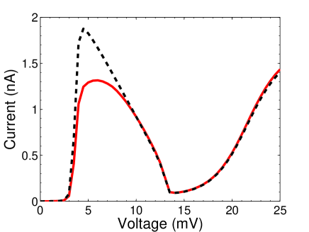
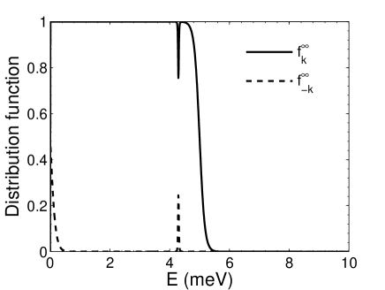
Figure 3: (Color online) I–V curve for the double-barrier tunneling structure, according to the expression (48) (solid curve) and the Landauer formula (49) (dashed curve) at 1 K.

Figure 4: Steady-state distribution functions (45) of the forward ($f^{\infty}_{k}$) and backward ($f^{\infty}_{-k}$) propagating states, at the peak voltage from Fig. 4 (5 meV) and 1 K. Energy is measured with respect to the bottom of the injector contact (Fig. 2). Significant deviations from the Fermi-Dirac equilibrium distributions in the contacts coincide with the peak in transmission.

V Summary and Concluding Remarks

In this paper, a simple theoretical description of the contact-induced decoherence in two-terminal nanostructures was provided within the framework of the open systems theory. The model active region – contact interaction was introduced to ensure proper carrier injection from the contacts. The steady-state statistical operator of the active region was calculated by relying on the Markovian map derived through coarse graining of the exact short time dynamics over the energy relaxation time of the bulk-like contacts. The ballistic-limit, steady state distribution functions of the forward and backward propagating states for a generic two-terminal nanostructure have been derived. The approach was illustrated on the example of a double-barrier tunneling structure, where an I-V curve that shows all the prominent resonant features was obtained. The relationship between the present approach and the Landauer-Büttiker formalism was addressed.

The inclusion of scattering within the active region would alter the form of $\mathcal{L}_{\mathrm{eff}}$, while scattering between the active region and the contacts (e.g. phonon-assisted tunneling) would essentially alter $\Lambda$. Equations (45) are the ballistic limit of the active region’s nonequilibrium steady-state distributions, and are a better starting point for transport calculations with scattering than the equilibrium distributions: for instance, the single-particle density matrix $\rho^{(1)}(k_{1},k_{2})=\mathrm{Tr}_{S}(d^{\dagger}_{k_{2}}d_{k_{1}}\rho_{S})$ in the ballistic limit is obviously diagonal, so to include scattering within the active region, one simple way would be to follow the single-particle density matrix formalism, Jacoboni (1992); Rossi and Jacoboni (1992); Brunetti et al. (1989); Hohenester and Pötz (1997); Ciancio et al. (2004); Platero and Aguado (2004) with the diagonal $\rho^{(1)}(k,k)$ specified by (45) as the ballistic limit. [Clearly, $\rho^{(1)}$ would no longer be diagonal in $k$ once scattering is included.] Scattering due to phonons within the active region is generally amenable to a weak-coupling approximation, so it can be treated as a perturbation within the Born approximation. To treat phonon-assisted injection from the contacts, the contact many-body Hilbert space can be augmented to formally include a tensor product of the contact and the phonon Hilbert spaces, Fischetti (1998, 1999) but again a simpler perturbative treatment may be enough. As for the treatment of electron-electron scattering, $\Lambda$ is in the form that allows for its inclusion between the active region and the contacts, but this is likely to be a difficult technical issue.

Finally, an important feature of the present approach is that it can be, at least in principle, extended to arbitrarily short timescales by forgoing the coarse-graining procedure, so non-Markovian effects can be observed. However, since the coarse-graining procedure phenomenologically accounts for the efficient electron-electron interaction in the contacts, without it we would be required to explicitly include this interaction in the contact Hamiltonian, which will require certain modifications to the present approach.

VI Acknowledgement

The author thanks D. K. Ferry, J. P. Bird, W. Pötz, and J. R. Barker for helpful discussions. This work has been supported by the NSF, award ECCS-0547415.

Appendix A Uncorrelated initial state and the existence of a subdynamics

In this Appendix, for an uncorrelated initial state of the form $\rho(0)=\rho_{E}\otimes\rho_{S}(0)$, we will explicitly show that $\rho_{2}(0)$, the component of $\rho(0)$ belonging to the zero eigenspace of $\overline{P}$, can be written in terms of $\rho_{S}(0)$ via equation (17), repeated here

$$\rho_{2}(0)=\mathcal{M}\rho_{1}(0)=d_{E}^{-\frac{1}{2}}\mathcal{M}\rho_{S}(0).$$ (50)

Together with (6), this equation proves that a subdynamics exists. We will explicitly derive the mapping $\mathcal{M}$ that is uniquely fixed by $\rho_{E}$.

A.1 Eigenbasis of $\overline{P}$

Let us first remind ourselves of the structure of the eigenspaces of $\overline{P}$. Its unit eigenspace is $d_{S}^{2}$-dimensional, spanned by vectors of the form

$$\left|\overline{\alpha\beta}\right\rangle=d_{E}^{-\frac{1}{2}}\sum_{i=1}^{d_{E}}\left|{i\alpha,i\beta}\right\rangle.$$ (51)

This form holds regardless of the environmental basis chosen, which is in agreement with the fact that the uniform environmental statistical operator $\overline{\rho}_{E}$ (the one that induces $\overline{P}$) is a scalar matrix, i.e., diagonal in any environmental basis. In the zero eigenspace of $\overline{P}$, for any choice of the environmental basis, we can identify two subspaces:

1) A subspace spanned by vectors of the form $\left|i\alpha,j\beta\right\rangle$, with $i\neq j$. This subspace is $d_{S}^{2}d_{E}(d_{E}-1)$-dimensional.

2) A subspace spanned by linear combinations of $\left|{i\alpha,i\beta}\right\rangle$, which are orthogonal to all $\left|\overline{\alpha\beta}\right\rangle$. These are given by

$$\left|b_{i,\alpha\beta}\right\rangle=\sqrt{\frac{d_{E}+1-i}{d_{E}-i}}\left(\left|{i\alpha,i\beta}\right\rangle-\frac{\sum_{j=i}^{d_{E}}\left|{j\alpha,j\beta}\right\rangle}{d_{E}+1-i}\right)$$ (52)

for every pair $\alpha,\beta$ and for $i=1,\dots,d_{E}-1$. This subspace is $d_{S}^{2}(d_{E}-1)$-dimensional. Note how the coefficients in the linear combinations do not depend on $\alpha,\beta$.

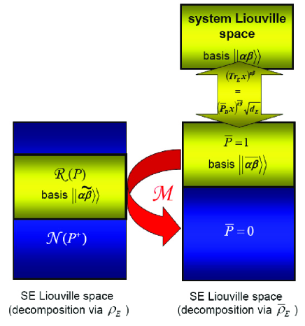
Figure 5: (Color online) Two decompositions of the total $SE$ Liouville space: the first one (right) is into the eigenspaces of $\overline{P}$, induced by the uniform statistical operator $\overline{\rho}_{E}$. (System Liouville space and $\overline{P}$’s unit eigenspace are equivalent.) The other decomposition is into $\mathcal{R}(P)$, the range of the projector $P$ induced by the initial environmental statistical operator $\rho_{E}$, and $\mathcal{N}(P^{\dagger})$, the null space of $P^{\dagger}$ and orthocomplement to $\mathcal{R}(P)$. These two decompositions enable us to construct the mapping $\mathcal{M}$ used in the reduced dynamics (19).

A.2 Range (Image Space) of $P$ and Null Space of $P^{\dagger}$

Now let us get back to the initially uncorrelated state of the form $\rho(0)=\rho_{E}\otimes\rho_{S}(0)$, and choose the eigenbasis of $\rho_{E}$ as the environmental basis $|j\rangle,j=1,\dots d_{E}$. $\rho_{E}$, the initial environmental statistical operator from $\rho(0)=\rho_{E}\otimes\rho_{S}(0)$ induces its own projection operator $P$, so that for any vector $\mu$ from the $SE$ Liouville space we can write

$$P\mu = \rho_{E}\otimes\left(\mathrm{Tr}_{E}\mu\right)$$ (53)

$$= \sum_{i,\alpha^{\prime},\beta^{\prime}}\rho_{E}^{i}\left(\sum_{k}\mu^{k\alpha^{\prime},k\beta^{\prime}}\right)\left|i\alpha,i\beta\right\rangle$$

The Latin indices $i,k=1,\dots d_{E}$ count environmental states, while the Greek ones $\alpha,\beta=1,\dots d_{S}$ count the system states. The essence of the following proof is to write any $P\mu$ in terms of the eigenvectors of $\overline{P}$, and then, since $P\rho(0)=\rho(0)$, draw important conclusions about its components $\rho_{2}(0)$ and $\rho_{S}(0)$.

$P$ is not Hermitian or diagonalizable. We can, however, still speak of its range (space of images) $\mathcal{R}(P)$, to which $\rho(0)$ belongs becaue $P\rho(0)=\rho(0)$. The orthocomplement to $\mathcal{R}(P)$ is $\mathcal{N}(P^{\dagger})$, the null space of the adjoint operator $P^{\dagger}$. It is easily noted that all vectors of the form $\left|i\alpha,j\beta\right\rangle$, with $i\neq j$, are in the null spaces of $\overline{P}$, $P$ and $P^{\dagger}$. Therefore, $\mathcal{N}(P^{\dagger})$ is at least $d_{S}^{2}d_{E}(d_{E}-1)$-dimensional. Where is the rest of $\mathcal{N}(P^{\dagger})$, i.e., what is a general form of a vector

$$\left|c_{q,\alpha\beta}\right\rangle=\sum_{i=1}^{d_{E}}\xi^{i}_{q}\left|i\alpha,i\beta\right\rangle,\quad(\forall\mu)\;\left\langle c_{q,\alpha\beta}|P\mu\right\rangle=0?$$ (54)

$$\left\langle c_{q,\alpha\beta}|P\mu\right\rangle = \sum_{i,j=1}^{d_{E}}(\xi^{i}_{q})^{*}\rho_{E}^{j}\left\langle i\alpha,i\beta|j\alpha^{\prime},j\beta^{\prime}\right\rangle(\mathrm{Tr}_{E}\mu)^{\alpha^{\prime}\beta^{\prime}},$$ (55)

$$= (\mathrm{Tr}_{E}\mu)^{\alpha^{\prime}\beta^{\prime}}\sum_{i=1}^{d_{E}}(\xi^{i})^{*}\rho_{E}^{j}$$

Therefore,

$$\left\langle c_{q,\alpha\beta}|P\mu\right\rangle=0\Longleftrightarrow\sum_{i=1}^{d_{E}}(\xi^{i}_{q})^{*}\rho_{E}^{i}=0$$ (56)

Columns $(\xi^{1}_{q},\dots\xi^{d_{E}}_{q})^{\mathrm{T}}$ satisfying (56) constitute a $d_{E}-1$-dimensional space, so we conclude that $\mathcal{N}(P^{\dagger})$ is of dimension $d_{S}^{2}d_{E}(d_{E}-1)+d_{S}^{2}(d_{E}-1)=d_{S}^{2}(d_{E}^{2}-1)$. Therefore, the rank of $P$ [dimension of $\mathcal{R}(P)$] is $d_{S}^{2}$, so it is isomorphic to the unit eigenspace of $\overline{P}$ and to the system Liouville space. One can show that the choice

$$\left|\widetilde{\alpha\beta}\right\rangle=\frac{1}{\sqrt{\mathrm{Tr}\rho_{E}^{2}}}\sum_{i=1}^{d_{E}}\rho_{E}^{i}\left|i\alpha,i\beta\right\rangle$$ (57)

indeed constitutes an orthonormal basis in $\mathcal{R}(P)$, and that

$$\left\langle\widetilde{\alpha\beta}|P\mu\right\rangle=0\quad{\mathrm{iff}}\quad\mathrm{Tr}_{E}\mu=0$$ (58a)

$$\left\langle\widetilde{\alpha\beta}|c_{q,\alpha^{\prime}\beta^{\prime}}\right\rangle=0,\quad\forall\alpha,\beta,q,\alpha^{\prime}\beta^{\prime}.$$ (58b)

Why was this analysis necessary? Because an uncorrelated initial state satisfies $P\rho(0)=\rho(0)$, which means the initial statistical operator belongs completely to $\mathcal{R}(P)$. Therefore, it can be written in terms of the basis $\left|\widetilde{\alpha\beta}\right\rangle$ as

$$\left\langle\widetilde{\alpha\beta}|\rho(0)\right\rangle=\mathrm{Tr}_{E}[\rho(0)]^{\alpha\beta}\sqrt{\mathrm{Tr}\rho_{E}^{2}}=\rho_{S}(0)^{\alpha\beta}\sqrt{\mathrm{Tr}\rho_{E}^{2}}.$$ (59)

In Fig. 5, mutual relationships among the eigenspaces of $\overline{P}$ and the null and image subspaces of $P$ are depicted. We obtain

$$\left\langle\overline{\alpha\beta}|\rho(0)\right\rangle=\left\langle\overline{\alpha\beta}|\widetilde{\alpha\beta}\right\rangle\left\langle\widetilde{\alpha\beta}|\rho(0)\right\rangle+\sum_{q}\left\langle\overline{\alpha\beta}|c_{q,\alpha\beta}\right\rangle\underbrace{\left\langle c_{q,\alpha\beta}|\rho(0)\right\rangle}_{=0}=\underbrace{\left\langle\overline{\alpha\beta}|\widetilde{\alpha\beta}\right\rangle}_{\frac{1}{\sqrt{d_{E}\mathrm{Tr}\rho_{E}^{2}}}}\underbrace{\left\langle\widetilde{\alpha\beta}|\rho(0)\right\rangle}_{\rho_{S}(0)^{\alpha\beta}\sqrt{\mathrm{Tr}\rho_{E}^{2}}}.$$ (60)

The important point to note is that $\left\langle\overline{\alpha\beta}|\rho(0)\right\rangle$ and $\left\langle\overline{\alpha\beta}|\rho(0)\right\rangle$ are equivalent up to the multiplicative constant $\left\langle\overline{\alpha\beta}|\widetilde{\alpha\beta}\right\rangle=\frac{1}{\sqrt{d_{E}\mathrm{Tr}\rho_{E}^{2}}}$.

We can now obtain the projection of $\rho_{2}(0)$ onto the zero-eigenspace of $\overline{P}$ as

$$\left\langle b_{j,\alpha\beta}|\rho(0)\right\rangle=\left\langle b_{j,\alpha\beta}|\widetilde{\alpha\beta}\right\rangle\left\langle\widetilde{\alpha\beta}|\rho(0)\right\rangle+\sum_{q}\left\langle b_{j\alpha\beta}|c_{q,\alpha\beta}\right\rangle\underbrace{\left\langle c_{q,\alpha\beta}|\rho(0)\right\rangle}_{=0}=\frac{\left\langle b_{j,\alpha\beta}|\widetilde{\alpha\beta}\right\rangle}{\left\langle\overline{\alpha\beta}|\widetilde{\alpha\beta}\right\rangle}\left\langle\overline{\alpha\beta}|\rho(0)\right\rangle\qquad$$ (61)

Since $\left\langle b_{i,\alpha\beta}|\widetilde{\alpha\beta}\right\rangle=\sqrt{\frac{d_{E}+1-i}{(d_{E}-i)Tr\rho_{E}^{2}}}\left(\rho_{E}^{i}-\frac{1}{d_{E}+1-i}\sum_{j=i}^{d_{E}}\rho_{E}^{j}\right)$, and $\left\langle\overline{\alpha\beta}|\widetilde{\alpha\beta}\right\rangle=\frac{1}{\sqrt{d_{E}\mathrm{Tr}\rho_{E}^{2}}}$, we arrive at

$$\left\langle b_{i,\alpha\beta}|\rho(0)\right\rangle=\mathcal{M}^{i}\left\langle\overline{\alpha\beta}|\rho(0)\right\rangle,\qquad\mathcal{M}^{i}=\sqrt{\frac{d_{E}(d_{E}+1-i)}{d_{E}-i}}\left(\rho_{E}^{i}-\frac{1}{d_{E}+1-i}\sum_{j=i}^{d_{E}}\rho_{E}^{j}\right).$$

Equations above fix the mapping $\rho_{2}(0)=\mathcal{M}\rho_{1}(0)$ from (50), and explicitly embody Lindblad’s argument on the existence of a subdynamics Lindblad (1996).

Appendix B Short-time decoherence in non-Markovian systems

In this Appendix, we formally show how to obtain the short-time limit to the exact completely positive non-Markovian dynamical map governing the evolution of $\rho_{S}$, in the form

$$\rho_{S}(t) = \mathrm{T^{c}}\exp\left[\int_{0}^{t}{\mathcal{K}}(t^{\prime})dt^{\prime}\right]\rho_{S}(0)$$

$$= \mathrm{T^{c}}\exp\left\{\int_{0}^{t}dt^{\prime}[-i{\mathcal{L}}_{\mathrm{{eff}}}(t^{\prime})-\mathcal{G}(t^{\prime})]\right\}\rho_{S}(0),$$

where ${\mathcal{L}}_{\mathrm{\mathrm{eff}}}(t)$ is a still undetermined effective Liouvillian, and $\mathcal{G}(t)$ is the dissipator term. It is well known that the form above holds for the dynamical semigroup in the Markov approximation, where the time-independent semigroup generator $-i\mathcal{L}_{\mathrm{eff}}-\mathcal{G}=\mathrm{const.}$ is of the well-known Lindblad form Lindblad (1976); Alicki and Lendi (1987) that ensures the map’s complete positivity.

Here, we will perform the short-time Taylor expansion of the exact equation (19) up to the second order in time

$$\rho_{S}(t)=\rho_{S}(0)+t\left(\frac{d\rho_{S}}{dt}\right)_{0}+\frac{t^{2}}{2}\left(\frac{d^{2}\rho_{S}}{dt^{2}}\right)_{0}+o(t^{3}),$$ (63)

and we will identify the terms in the first and second derivatives from the desired equation (B)

$$\left(\frac{d\rho_{S}}{dt}\right)_{0} = \left[-i{\mathcal{L}}_{\mathrm{{eff}}}(0)-\mathcal{G}(0)\right]\rho_{S}(0),$$ (64a)

$$\left(\frac{d^{2}\rho_{S}}{dt^{2}}\right)_{0} = \left[-i\left(\frac{d\mathcal{L}_{\mathrm{eff}}}{dt}\right)_{0}-\left(\frac{d\mathcal{G}}{dt}\right)_{0}\right]\rho_{S}(0)$$ (64b)

$$+ \left[-i{\mathcal{L}}_{\mathrm{{eff}}}(0)-\mathcal{G}(0)\right]^{2}\rho_{S}(0).$$

with those obtained from the exact evolution described by Eq. (19).

Indeed, by using the initial conditions $R(0)=0$ and $\mathcal{V}(0,0)=1$ given in Eq. (14), from Eq. (19) we directly obtain

$$\left(\frac{d\rho_{S}}{dt}\right)_{0} = -i\left({\mathcal{L}}_{11}+{\mathcal{L}}_{12}\mathcal{M}\right)\rho_{S}(0)$$ (65)

$$= -i\left[{\mathcal{H}}_{S}+\langle{{\mathcal{H}}_{\mathrm{{int}}}}\rangle,\rho_{S}(0)\right].$$

Here, we have used the facts that ${\mathcal{L}}_{11}$ is generated by the Hamiltonian ${\mathcal{H}}_{S}+\overline{\mathcal{H}}_{\mathrm{{int}}}$, where $\overline{\mathcal{H}}_{\mathrm{{int}}}=\mathrm{Tr}_{E}({\mathcal{H}}_{\mathrm{{int}}})/d_{E}$, while ${\mathcal{L}}_{12}\mathcal{M}$ is generated by the Hamiltonian $\langle{\mathcal{H}}_{\mathrm{{int}}}\rangle-\overline{\mathcal{H}}_{\mathrm{{int}}}$, where $\langle{\mathcal{H}}_{\mathrm{{int}}}\rangle=\mathrm{Tr}_{E}\left(\rho_{E}{\mathcal{H}}_{\mathrm{{int}}}\right)$ is the averaged interaction Hamiltonian (see Appendix B.1). Consequently,

$$\mathcal{L}_{\mathrm{eff}}(0)={\mathcal{L}}_{11}+{\mathcal{L}}_{12}\mathcal{M} = \left[{\mathcal{H}}_{S}+\langle{{\mathcal{H}}_{\mathrm{{int}}}}\rangle,\dots\right],$$ (66a)

$$\mathcal{G}(0) = 0.\hfill$$ (66b)

Taking the first derivative of Eq. (19) and employing $R(0)=0$, $\left(\frac{dR}{dt}\right)_{0}=i{\mathcal{L}}_{21}$, $\mathcal{V}(0,0)=1$, and $\left[\frac{d\mathcal{V}(t,0)}{dt}\right]_{0}=i{\mathcal{L}}_{22}$ [Eq. (14)], we directly obtain

$$\left(\frac{d^{2}\rho_{S}}{dt^{2}}\right)_{0}= - \left({\mathcal{L}}_{12}{\mathcal{L}}_{21}+{\mathcal{L}}_{12}{\mathcal{L}}_{22}\mathcal{M}\right)\rho_{S}(0)$$ (67)

$$- {\mathcal{L}}_{11}\left({\mathcal{L}}_{11}+{\mathcal{L}}_{12}\mathcal{M}\right)\rho_{S}(0).$$

After subtracting $[-i\mathcal{L}_{\mathrm{eff}}(0)]^{2}\rho_{S}(0)$ from $\left(\frac{d^{2}\rho_{S}}{dt^{2}}\right)_{0}$, what we obtain is action of the operator $-i\left(\frac{d{\mathcal{L}}_{\mathrm{{eff}}}}{dt}\right)_{0}-\left(\frac{d\mathcal{G}}{dt}\right)_{0}$ on $\rho_{S}(0)$. Therefore, we will introduce operator $\Lambda$ as

$$2\Lambda \equiv i\left(\frac{d{\mathcal{L}}_{\mathrm{{eff}}}}{dt}\right)_{0}+\left(\frac{d\mathcal{G}}{dt}\right)_{0},$$ (68)

where

$$2{\Lambda} = ({\mathcal{L}}_{12}{\mathcal{L}}_{21}+{\mathcal{L}}_{12}{\mathcal{L}}_{22}\mathcal{M})-{\mathcal{L}}_{12}\mathcal{M}\left({\mathcal{L}}_{11}+{\mathcal{L}}_{12}\mathcal{M}\right).$$

Operator ${\Lambda}$ contains essential information on the directions of coherence loss in both non-Markovian and Markovian systems. After a straightforward calculation, documented in Appendix B.1, one can obtain the matrix elements of $\Lambda$ in the tensor-product basis of the system Liouville space

$${\Lambda}^{\alpha\beta}_{\alpha^{\prime}\beta^{\prime}} = \frac{1}{2}\sum_{k}\rho_{E}^{k}\left\{\left({\mathcal{H}}_{\mathrm{int}}^{2}\right)^{k\alpha}_{k\alpha^{\prime}}\delta^{\beta^{\prime}}_{\beta}-2\sum_{k^{\prime}}\left({\mathcal{H}}_{\mathrm{int}}\right)^{k^{\prime}\alpha}_{k\alpha^{\prime}}\left({\mathcal{H}}_{\mathrm{int}}\right)^{k\beta^{\prime}}_{k\beta}+\left({\mathcal{H}}_{\mathrm{int}}^{2}\right)^{k\beta^{\prime}}_{k\beta^{\prime}}\delta^{\alpha}_{\alpha^{\prime}}\right\}$$ (69)

$$- \frac{1}{2}\left\{\left(\langle{\mathcal{H}}_{\mathrm{int}}\rangle^{2}\right)^{\alpha}_{\alpha^{\prime}}\delta^{\beta^{\prime}}_{\beta}-2\langle{\mathcal{H}}_{\mathrm{int}}\rangle^{\alpha}_{\alpha^{\prime}}\langle{\mathcal{H}}_{\mathrm{int}}\rangle^{\beta^{\prime}}_{\beta}+\left(\langle{\mathcal{H}}_{\mathrm{int}}\rangle^{2}\right)^{\beta^{\prime}}_{\beta}\delta^{\alpha}_{\alpha^{\prime}}\right\},$$

where, for simplicity, the environmental basis is assumed to be the eigenbasis of the environment initial statistical operator $\rho_{E}$. In a more compact form, the action of ${\Lambda}$ on any vector $\mu_{S}$ from the system Liouville space can be given as

$${\Lambda}\mu_{S} = \frac{1}{2}\mathrm{Tr_{E}}\left\{\left(\rho_{E}\otimes\mu_{S}\right){\mathcal{H}}_{\mathrm{{int}}}{\mathcal{H}}_{\mathrm{{int}}}-2{\mathcal{H}}_{\mathrm{{int}}}\left(\rho_{E}\otimes\mu_{S}\right){\mathcal{H}}_{\mathrm{{int}}}+{\mathcal{H}}_{\mathrm{{int}}}{\mathcal{H}}_{\mathrm{{int}}}\left(\rho_{E}\otimes\mu_{S}\right)\right\}$$ (70)

$$- \frac{1}{2}\left\{\mu_{S}\langle{\mathcal{H}}_{\mathrm{int}}\rangle\langle{\mathcal{H}}_{\mathrm{int}}\rangle-2\langle{\mathcal{H}}_{\mathrm{int}}\rangle\mu_{S}\langle{\mathcal{H}}_{\mathrm{int}}\rangle+\langle{\mathcal{H}}_{\mathrm{int}}\rangle\langle{\mathcal{H}}_{\mathrm{int}}\rangle\mu_{S}\right\}$$

An interaction Hamiltonian can always be written as

$${\mathcal{H}}_{\mathrm{int}}=\sum_{i}^{i_{\mathrm{max}}}f_{i}\otimes\varphi_{i},$$

where $f_{i}$ are Hermitian operators on the environment Hilbert space, while $\varphi_{i}$ are Hermitian operators on the system Hilbert space. With this form of the interaction in mind, one can write compactly

$${\Lambda}\mu_{S} = \frac{1}{2}\sum_{i,j}\left(\langle f_{i}f_{j}^{\dagger}\rangle-\langle f_{i}\rangle\langle f_{j}^{\dagger}\rangle\right)\left\{\varphi_{i}\varphi_{j}^{\dagger}\mu_{S}-2\varphi_{j}^{\dagger}\mu_{S}\varphi_{i}+\mu_{S}\varphi_{i}\varphi_{j}^{\dagger}\right\}$$ (71)

$$= -\frac{1}{2}\sum_{i,j}\left(\langle f_{i}f_{j}^{\dagger}\rangle-\langle f_{i}\rangle\langle f_{j}^{\dagger}\rangle\right)\left\{\left[\varphi_{i},\mu_{S}\varphi_{j}^{\dagger}\right]+\left[\varphi_{i}\mu_{S},\varphi_{j}^{\dagger}\right]\right\}$$

where, as before, $\langle\dots\rangle=\mathrm{Tr}_{E}(\rho_{E}\dots)$.

¿From its definition (68), operator $\Lambda$ satisfies $2\Lambda=i\left(\frac{d{\mathcal{L}}_{\mathrm{{eff}}}}{dt}\right)_{0}+\left(\frac{d\mathcal{G}}{dt}\right)_{0}.$ If we look at the matrix elements of the matrix [Eq. (71)]

$$m_{ij}=\langle f_{i}f_{j}^{\dagger}\rangle-\langle f_{i}\rangle\langle f_{j}^{\dagger}\rangle,$$

we immediately note that $m_{ij}=m_{ji}^{*}$ due to the hermiticity of $f^{\prime}s$. As a result,

$$\frac{d{\mathcal{L}}_{\mathrm{{eff}}}}{dt}=0,\quad\Lambda=\frac{1}{2}\left(\frac{d\mathcal{G}}{dt}\right)_{0}.$$ (72)

Furthermore, $m$ is a positive-definite matrix, since for any complex $i_{max}$ column $c=(c_{1},\dots,c_{i_{max}})^{\mathrm{T}}$ it holds

$$\langle c|m|c\rangle = \sum_{i,j}c^{i*}m_{ij}c^{j}=\sum_{i,j}c^{i*}\left\{\langle f_{i}f_{j}^{\dagger}\rangle-\langle f_{i}\rangle\langle f_{j}^{\dagger}\rangle\right\}c^{j}$$

$$= \sum_{i,j}\mathrm{Tr}_{E}\left\{\rho_{E}\left(c^{i*}f_{i}\right)\left(c^{j*}f_{j}\right)^{\dagger}\right\}-\mathrm{Tr}_{E}\left(\rho_{E}c^{i*}f_{i}\right)\mathrm{Tr}_{E}\left(\rho_{E}c^{j*}f_{j}\right)^{*}$$

$$= \mathrm{Tr}_{E}\left\{\rho_{E}\left(\sum_{i}c^{i*}f_{i}\right)\left(\sum_{i}c^{i*}f_{i}\right)^{\dagger}\right\}-\left|\mathrm{Tr}_{E}\left\{\rho_{E}\left(\sum_{i}c^{i*}f_{i}\right)\right\}\right|^{2}\geq 0.$$

The last inequality can be obtained by noting that, for any matrix $a$,

$$\mathrm{Tr}_{E}\left(\rho_{E}aa^{\dagger}\right) = \sum_{k,k^{\prime}}\rho_{E}^{k}\left|a^{k^{\prime}}_{k}\right|^{2}\geq\sum_{k}\rho_{E}^{k}\left|a^{k}_{k}\right|^{2}$$

$$\geq \sum_{k}(\rho_{E}^{k})^{2}\left|a^{k}_{k}\right|^{2}\geq\left|\sum_{k}\rho_{E}^{k}a^{k}_{k}\right|^{2}$$

$$= \left|\mathrm{Tr}_{E}\left(\rho_{E}a\right)\right|^{2}.$$

As a result, we conclude that $-\Lambda$ has the form expected from the Lindblad dissipator (it has the units of $t^{-2}$, though, unlike the Lindblad dissipator that has the units of $t^{-1}$).

Up to the second order in time, the generator $\mathcal{K}$ of the non-Markovian map (18) can now be approximated as

$$\mathcal{K}(t)\approx-i\mathcal{L}_{\mathrm{eff}}-2\Lambda t+o(t^{2}),$$ (75)

where $\mathcal{L}_{\mathrm{eff}}\equiv\mathcal{L}_{\mathrm{eff}}(0)$ from Eq. (66a), and $\Lambda$ is given in Eq. (69).

B.1 How to calculate ${\mathcal{L}}_{12}\mathcal{M}$ and ${\Lambda}$

${\mathcal{L}}_{12}\mathcal{M}$ can be found as

$$\left({\mathcal{L}}_{12}\mathcal{M}\right)^{\overline{\alpha\beta}}_{\overline{\alpha^{\prime}\beta^{\prime}}}=\sum_{j=1}^{d_{E}-1}\left\langle\overline{\alpha\beta}|L|b_{j,\alpha^{\prime}\beta^{\prime}}\right\rangle\mathcal{M}^{j}=\sum_{j=1}^{d_{E}-1}\left\langle\overline{\alpha\beta}|L|b_{j,\alpha^{\prime}\beta^{\prime}}\right\rangle\frac{\left\langle b_{j,\alpha^{\prime}\beta^{\prime}}|\widetilde{\alpha^{\prime}\beta^{\prime}}\right\rangle}{\left\langle\overline{\alpha^{\prime}\beta^{\prime}}|\widetilde{\alpha^{\prime}\beta^{\prime}}\right\rangle}$$ (76)

For a fixed $\alpha,\beta$, there is a $d_{E}$-dimensional space spanned by all $|i\alpha,i\beta\rangle$. A unit operator in this space can be written as $\sum_{i=1}^{d_{E}-1}\left|b_{i,\alpha\beta}\right\rangle\left\langle b_{i,\alpha\beta}\right|+\left|\overline{\alpha\beta}\right\rangle\left\langle\overline{\alpha\beta}\right|=1_{\alpha\beta}$

$$\left({\mathcal{L}}_{12}\mathcal{M}\right)^{\overline{\alpha\beta}}_{\overline{\alpha^{\prime}\beta^{\prime}}} = \sum_{j=1}^{d_{E}-1}\left\langle\overline{\alpha\beta}|L|b_{j,\alpha^{\prime}\beta^{\prime}}\right\rangle\mathcal{M}^{j}=\left\langle\overline{\alpha\beta}|L\left(1_{\alpha^{\prime}\beta^{\prime}}-\left|\overline{\alpha^{\prime}\beta^{\prime}}\right\rangle\left\langle\overline{\alpha^{\prime}\beta^{\prime}}\right|\right)|\widetilde{\alpha^{\prime}\beta^{\prime}}\right\rangle\frac{1}{\left\langle\overline{\alpha^{\prime}\beta^{\prime}}|\widetilde{\alpha^{\prime}\beta^{\prime}}\right\rangle}$$

$$= \frac{\left\langle\overline{\alpha\beta}|L|\widetilde{\alpha^{\prime}\beta^{\prime}}\right\rangle}{\left\langle\overline{\alpha^{\prime}\beta^{\prime}}|\widetilde{\alpha^{\prime}\beta^{\prime}}\right\rangle}-\left\langle\overline{\alpha\beta}|L|\overline{\alpha^{\prime}\beta^{\prime}}\right\rangle=\sum_{i,j=1}^{d_{E}}\langle{i\alpha,i\beta}|L|{j\alpha^{\prime},j\beta^{\prime}}\rangle\left(\rho_{E}^{j}-\frac{1}{d_{E}}\right)$$

$$= \sum_{i=1}^{d_{E}}\left(h^{i\alpha}_{i\alpha^{\prime}}\delta^{\beta}_{\beta^{\prime}}-h^{i\beta^{\prime}}_{i\beta}\delta^{\alpha}_{\alpha^{\prime}}\right)\left(\rho_{E}^{i}-\frac{1}{d_{E}}\right)$$

$$= \sum_{i=1}^{d_{E}}\left[({\mathcal{H}}_{\mathrm{int}})^{i\alpha}_{i\alpha^{\prime}}\delta^{\beta}_{\beta^{\prime}}-({\mathcal{H}}_{\mathrm{int}})^{i\beta^{\prime}}_{i\beta}\delta^{\alpha}_{\alpha^{\prime}}\right]\left(\rho_{E}^{i}-\frac{1}{d_{E}}\right).$$

The last line is easily obtained by showing that the contributions from the environment Hamiltonian [$({\mathcal{H}}_{\mathrm{{env}}})^{i\alpha}_{i\beta}=({\mathcal{H}}_{E})^{i}_{i}\delta^{\alpha}_{\beta}$] and from the system Hamiltonian [$({\mathcal{H}}_{\mathrm{{sys}}})^{i\alpha}_{i\beta}=({\mathcal{H}}_{S})^{\alpha}_{\beta}$] vanish.

When one deals with interaction Hamiltonians of the hopping type, i.e., those that contain an odd number of environmental creation/annihilation operators and therefore necessarily alter the environmental state, all $({\mathcal{H}}_{\mathrm{int}})^{i\alpha}_{i\alpha^{\prime}}=0$, and clearly ${\mathcal{L}}_{12}\mathcal{M}=0$, which we used in Sec. C. Also, when the statistical operator is uniform ($\rho_{E}=\overline{\rho}_{E}$), ${\mathcal{L}}_{12}\mathcal{M}=0$. Note how this term accounts for the information influx from the environment, because it captures the deviation of the environment statistical operator from the uniform statistical operator (the uniform statistical operator carries the maximum information entropy, i.e., environment has no information to transmit).

In order to calculate $\Lambda$, which was defined as $2\Lambda={\mathcal{L}}_{12}{\mathcal{L}}_{21}+{\mathcal{L}}_{12}{\mathcal{L}}_{22}\mathcal{M}-{\mathcal{L}}_{12}\mathcal{M}\left({\mathcal{L}}_{11}+{\mathcal{L}}_{12}\mathcal{M}\right)$ in Eq. (68), we should first note that ${\mathcal{L}}_{12}\mathcal{M}\left({\mathcal{L}}_{11}+{\mathcal{L}}_{12}\mathcal{M}\right)$ is commutator generated, i.e.,

$${\mathcal{L}}_{12}\mathcal{M}\left({\mathcal{L}}_{11}+{\mathcal{L}}_{12}\mathcal{M}\right)=\left[\langle{\mathcal{H}}_{\mathrm{int}}\rangle-\overline{\mathcal{H}}_{\mathrm{int}},\left[{\mathcal{H}}_{S}+\langle{\mathcal{H}}_{\mathrm{int}}\rangle,\dots\right]\right].$$

The term ${\mathcal{L}}_{12}{\mathcal{L}}_{21}+{\mathcal{L}}_{12}{\mathcal{L}}_{22}\mathcal{M}$ can be rewritten as

$$\left({\mathcal{L}}_{12}{\mathcal{L}}_{21}+{\mathcal{L}}_{12}{\mathcal{L}}_{22}\mathcal{M}\right)^{\alpha\beta}_{\alpha^{\prime}\beta^{\prime}} = \langle\overline{\alpha\beta}|L^{2}-L\overline{P}L|\widetilde{\alpha^{\prime}\beta^{\prime}}\rangle\frac{1}{\langle\overline{\alpha^{\prime}\beta^{\prime}}|\widetilde{\alpha^{\prime}\beta^{\prime}}\rangle}$$

$$= \langle\overline{\alpha\beta}|L^{2}|\widetilde{\alpha^{\prime}\beta^{\prime}}\rangle\frac{1}{\langle\overline{\alpha^{\prime}\beta^{\prime}}|\widetilde{\alpha^{\prime}\beta^{\prime}}\rangle}-\sum_{\gamma,\sigma=1}^{d_{S}}\langle\overline{\alpha\beta}|L|\overline{\gamma\sigma}\rangle\langle\overline{\gamma\sigma}|L|\widetilde{\alpha^{\prime}\beta^{\prime}}\rangle\frac{1}{\langle\overline{\alpha^{\prime}\beta^{\prime}}|\widetilde{\alpha^{\prime}\beta^{\prime}}\rangle}$$

$$= \sum_{i,j=1}^{d_{E}}\langle i\alpha,i\beta|L^{2}|j\alpha^{\prime},j\beta^{\prime}\rangle\rho_{E}^{j}$$

$$- \frac{1}{d_{E}}\sum_{i,j,k=1}^{d_{E}}\sum_{\gamma,\sigma=1}^{d_{S}}\rho_{E}^{j}\langle i\alpha,i\beta|L|k\gamma,k\sigma\rangle\langle k\gamma,k\sigma|L|j\alpha^{\prime},j\beta^{\prime}\rangle,$$

where the eigenbasis of the environment initial statistical operator $\rho_{E}$ is chosen to be the environmental basis. Upon a straightforward (and somewhat lengthy) calculation, with the only constraint being that $[\rho_{E},{\mathcal{H}}_{E}]=0$, which is typically satisfied, we obtain Eq. (69).

Appendix C Two Additional Examples

The following two examples serve to illustrate that the usefulness of the coarse-grained map (27) may extend beyond the strict validity specified by (29), and may offer a particularly simple way to identify the steady state alone from first principles.

The first example (C.1) is analytically solvable and possesses the long-time Markovian evolution regardless of the interaction strength. We show here that there exists a mathematical coarse-graining time $\tau$, shorter than any other timescale in the system or environment, so that the exact long-time Markovian evolution coincides with that obtained from the short-time evolution by coarsening over $\tau$ (27).

On the second example (C.2), we show that relaxation towards the correct equilibrium state is easily obtained by using (27) (or equivalently by employing Theorem 2 in Sec. III).

C.1 Spin-boson model with pure dephasing

One of the few analytically solvable Lidar et al. (2001); Palma et al. (1996); Duan and Guo (1998); Grifoni et al. (1997); Thorwart et al. (2004); Emary and Brandes (2004) open system problems is that of a two-level system coupled to a dephasing-only boson bath, with the relevant Hamiltonians are given by

$${\mathcal{H}}_{S} = \frac{\omega}{2}\sigma_{z},\;{\mathcal{H}}_{E}=\sum_{\vec{q}}\Omega_{q}\left(b^{\dagger}_{\vec{q}}b_{\vec{q}}+\frac{1}{2}\right),$$

$${\mathcal{H}}_{\mathrm{int}} = \sum_{\vec{q}}\sigma_{z}\left\{g(\Omega_{\vec{q}})b_{\vec{q}}+g(\Omega_{\vec{q}})^{*}b_{\vec{q}}^{\dagger}\right\}.$$ (79)

Here, $\sigma_{z}$ is the Pauli matrix, $b_{\vec{q}}^{\dagger}$ and $b_{\vec{q}}$ and the boson creation and annihilation operators of the $q$-th boson mode, respectively, $\pm\omega/2$ are the system energy levels (divided by $\hbar$), and $\Omega_{q}$ is the boson mode frequency. The boson modes are initially in a thermal state with $\langle n_{q}\rangle=\langle b^{\dagger}_{q}b_{q}\rangle=\frac{1}{\exp(\hbar\Omega_{q}/k_{B}T)-1}$. Because of the interaction linear in environment creation/annihilation operators, $\langle\mathcal{H}_{\mathrm{int}}\rangle=0$, so ${\mathcal{L}}_{S}={\mathcal{L}}_{\mathrm{eff}}$:

$${\mathcal{L}}_{\mathrm{eff}}={\mathcal{L}}_{S}=\omega\left[\begin{array}[]{cccc}0&0&0&0\\ 0&1&0&0\\ 0&0&-1&0\\ 0&0&0&0\end{array}\right],$$ (84)

where the rows/columns are ordered as $1=\left|+\right\rangle\left<+\right|,2=\left|+\right\rangle\left<-\right|,3=\left|-\right\rangle\left<+\right|,4=\left|-\right\rangle\left<-\right|$ ($\pm$ refer to the positive/negative (upper/lower) energy state). Operator $\Lambda$ can be calculated according to (69) as

$${\Lambda} = {\lambda_{d}}\left[\begin{array}[]{cccc}0&0&0&0\\ 0&1&0&0\\ 0&0&1&0\\ 0&0&0&0\end{array}\right],$$ (89)

$${\lambda_{d}} = 2\sum_{\vec{q}}|g(\Omega_{\vec{q}})|^{2}\coth{\left(\frac{\hbar\Omega_{q}}{2k_{B}T}\right)}$$ (90)

$$= 2\int_{0}^{\infty}d\Omega\mathcal{D}(\Omega)|g(\Omega)|^{2}\coth{\left(\frac{\hbar\Omega}{2k_{B}T}\right)},$$

where $\mathcal{D}(\Omega)$ is the density of boson states.

${\mathcal{L}}_{S}$ and ${\Lambda}$ obviously commute, and their common zero eigenspace [$\mathcal{N}(\Lambda)=\mathcal{N}({\mathcal{L}}_{\mathrm{eff}})$] contains all density matrices with zero off-diagonal elements. This means that, for a given initial statistical operator, the off-diagonal matrix elements will decay to zero while the diagonal elements remain unchanged:

$$\left[\rho_{S}(t)\right]_{++} = \left[\rho_{S}(0)\right]_{++},\;\left[\rho_{S}(t)\right]_{--}=\left[\rho_{S}(0)\right]_{--},$$

$$\left[\rho_{S}(t)\right]_{+-} = \left[\rho_{S}(0)\right]_{+-}e^{-i\omega t-\lambda_{d}\tau t},$$ (91)

$$\left[\rho_{S}(t)\right]_{-+} = \left[\rho_{S}(0)\right]_{-+}e^{+i\omega t-\lambda_{d}\tau t},$$

The steady state will be determined by simply annulling the off-diagonal elements. This is the correct steady state, as shown in the exact solution Breuer and Petruccione (2002).

Instead of $\exp(-\lambda_{d}\tau t)$, in the exact solution decoherence is seen through the term $\exp[-\Gamma(t)]$, where the $\Gamma(t)$, the decoherence exponent, behaves as

$$\Gamma(t)=\int_{0}^{\infty}d\Omega 2\mathcal{D}(\Omega)|g(\Omega)|^{2}\coth{\left(\frac{\hbar\Omega}{2k_{B}T}\right)}\frac{\sin^{2}(\Omega t/2)}{(\Omega/2)^{2}}.$$ (92)

For short-times, $\Gamma(t)\approx\lambda_{d}t^{2}$, as should be expected, because we know our expansion (23) is exact up to the second order in time. In the long-time limit for $\Gamma(t)$, only the low frequency contributions survive, since $\lim_{t\rightarrow\infty}\frac{\sin^{2}(\Omega t/2)}{(\Omega/2)^{2}t}=\pi\delta(\Omega)$, so

$$\Gamma(t\rightarrow\infty)=t\lim_{\Omega\rightarrow 0}2\pi\mathcal{D}(\Omega)|g(\Omega)|^{2}\coth{\left(\frac{\hbar\Omega}{2k_{B}T}\right)}.$$ (93)

We need to match this long-time behavior of $\Gamma(t)$ with our coarse-grained term $\lambda_{d}\tau t$, in order to obtain $\tau$.

$$\tau=\lim_{t\rightarrow\infty}\frac{\Gamma(t)}{\lambda_{d}t}=\frac{\lim_{\Omega\rightarrow 0}2\pi\mathcal{D}(\Omega)|g(\Omega)|^{2}\coth{\left(\frac{\hbar\Omega}{2k_{B}T}\right)}}{2\int_{0}^{\infty}d\Omega\mathcal{D}(\Omega)|g(\Omega)|^{2}\coth{\left(\frac{\hbar\Omega}{2k_{B}T}\right)}}.$$ (94)

Let us consider the example of an Ohmic bath (e.g., page 228 of Ref. Breuer and Petruccione, 2002), with $D(\Omega)|g(\Omega)|^{2}=\frac{1}{4}\Omega\exp(-\Omega/\Omega_{c})$ and $\Omega_{c}$ being a density-of-states cutoff frequency. Typically, $\hbar\Omega_{c}\gg k_{B}T$. In the numerator, one can approximate $\coth{\left(\frac{\hbar\Omega}{2k_{B}T}\right)}\approx\frac{2k_{B}T}{\hbar\Omega}$, while the $\coth{}$ function in the denominator is always greater than 1, yielding

$$\tau<\left(\frac{k_{B}T}{\hbar\Omega_{C}}\right)\frac{2\pi}{\Omega_{c}}\ll\frac{2\pi}{\Omega_{c}}.$$ (95)

Being typically the largest frequency scale in the full $SE$ problem, $\Omega_{c}$ sets the shortest physical timescale. Clearly, $\tau$ is even shorter than the period associated with $\Omega_{c}$, which justifies our use of the short-time expansion and subsequent coarse-graining.

Note the long-time behavior $\exp(-t/\tau_{T})$ of the decoherence term $\Gamma$, where $\tau_{T}=\hbar/\pi k_{B}T$ is the thermal correlation time. However, our time $\tau$ is the mathematical coarse-graining time, which is very short. The relationship between the correct physical correlation loss time and the mathematically appropriate time is

$$\tau=(\lambda_{d}\tau_{T})^{-1}.$$ (96)

C.2 Jaynes-Cummings model in the rotating wave approximation

The Jaynes-Cummings Hamiltonian in the rotating-wave approximation Jaynes and Cummings (1963); Meystre and Wright (1988); Hussin and Nieto (2005); van Wonderen and Lendi (1995) describes the decay of a two-level system in the presence of a single boson mode of resonant frequency. The relevant Hamiltonians are

$${\mathcal{H}}_{S} = \frac{1}{2}\omega\sigma_{z},\;{\mathcal{H}}_{E}=\omega\left(b^{\dagger}b+\frac{1}{2}\right),$$

$${\mathcal{H}}_{\mathrm{int}} = g\left(b^{\dagger}\sigma_{-}+b\sigma_{+}\right).$$ (97)

Here, $\sigma_{z},$ $\sigma_{+}=\left(\sigma_{x}+i\sigma_{y}\right)/e$, and $\sigma_{-}=\left(\sigma_{x}-i\sigma_{y}\right)/2$ are the Pauli matrices, $b^{\dagger}$ and $b$ are the boson creation and annihilation operators, respectively, $\pm\omega/2$ are the system energy levels (in units of frequency) and $\omega$ is also the boson mode frequency, and $g$ is a parameter measuring the interaction strength. The boson mode is initially in a thermal state with $\langle n\rangle=\langle b^{\dagger}b\rangle=\frac{1}{\exp(\hbar\omega/k_{B}T)-1}$. As in the spin-boson example, ${\mathcal{L}}_{\mathrm{eff}}={\mathcal{L}}_{S}$ because of the interaction linear in environment creation/annihilation operators:

$${\mathcal{L}}_{\mathrm{eff}}={\mathcal{L}}_{S}=\omega\left[\begin{array}[]{cccc}0&0&0&0\\ 0&1&0&0\\ 0&0&-1&0\\ 0&0&0&0\end{array}\right].$$ (102)

Operator $\Lambda$ can be calculated according to Equation (69) as

$${\Lambda}=\frac{g^{2}}{2}\left[\begin{array}[]{cccc}2\langle n\rangle+2&0&0&-2\langle n\rangle\\ 0&2\langle n\rangle+1&0&0\\ 0&0&2\langle n\rangle+1&0\\ -2\langle n\rangle-2&0&0&2\langle n\rangle\end{array}\right].$$ (107)

${\mathcal{L}}_{S}$ and ${\Lambda}$ commute, and we immediately note two common one-dimensional eigenspaces: $\rho_{+-}$ is associated with the ${\mathcal{L}}_{S}$ and ${\Lambda}$ eigenvalues $\omega$ and $g^{2}(2\langle n\rangle+1)/2$, respectively, while $\rho_{-+}$ is associated with the eigenvalues $-\omega$ and $g^{2}(2\langle n\rangle+1)/2$.

On the other hand, the space spanned by $|+\rangle\langle+|$ and $|-\rangle\langle-|$ is the null space of ${\mathcal{L}}_{\mathrm{eff}}$. Solving the eigenproblem of ${\Lambda}$ reduced to this space gives

$$\det\left[\begin{array}[]{cc}g^{2}\left(\langle n\rangle+1\right)-\lambda&-g^{2}\langle n\rangle\\ -g^{2}\left(\langle n\rangle+1\right)&g^{2}\langle n\rangle-\lambda\end{array}\right]=0,$$ (110)

$$\lambda=0\quad\mathrm{and}\quad\lambda=\lambda_{d}\equiv g^{2}\left(2\langle n\rangle+1\right).$$

An eigenvector $\mu^{0}=(\mu^{0}_{++},\mu^{0}_{--})^{\mathrm{T}}$ corresponding to the zero eigenvalue of the matrix $\Lambda$ is characterized by

$$\mu^{0}_{--}=\mu^{0}_{++}\frac{\langle n\rangle+1}{\langle n\rangle}.$$ (111)

If we are looking for a statistical operator that belongs to the zero eigenspace of $\Lambda$, it also has to satisfy the constraint of the unit trace, which fixes

$$\mu^{0}_{++}=\frac{\langle n\rangle}{2\langle n\rangle+1},\quad\mu^{0}_{--}=\frac{\langle n\rangle+1}{2\langle n\rangle+1}.$$ (112)

One recognizes these components as the thermal equilibrium values of the population of the upper and lower level of our two-level system, respectively (see, for instance, p. 149 of Ref. Breuer and Petruccione, 2002). Therefore, by seeking the steady state in $\mathcal{N}(\Lambda)\cap\mathcal{N}({\mathcal{L}}_{\mathrm{eff}})$, we have obtained the physically correct result.

References

- Jacoboni and Reggiani (1983) C. Jacoboni and L. Reggiani, Rev. Mod. Phys. 65, 645 (1983).
- Pötz (1989) W. Pötz, J. Appl. Phys. 66, 2458 (1989).
- Frensley (1990) W. R. Frensley, Rev. Mod. Phys. 62, 745 (1990).
- Bird et al. (2003) J. P. Bird, R. Akis, D. K. Ferry, A. P. S. de Moura, Y. C. Lai, and K. M. Indlekofer, Rep. Prog. Phys. 66, 583 (2003).
- Elhassan et al. (2005) M. Elhassan, J. P. Bird, R. Akis, D. K. Ferry, T. Ida, and K. Ishibashi, J. Phys.: Condens. Matter 17, L351 (2005).
- Grubin and Ferry (1998) H. L. Grubin and D. K. Ferry, Semicond. Sci. Tech. 13 (8A), Suppl. S, A44 (1998).
- Ferry et al. (2003) D. K. Ferry, R. Akis, J. P. Bird, M. Elhassan, I. Knezevic, C. Prasad, and A. Shailos, J. Vac. Sci. Technol. B 21, 1891 (2003).
- Svizhenko and Anantram (2003) A. Svizhenko and M. P. Anantram, IEEE Trans. Electron. Dev. 50, 1459 (2003).
- Knezevic and Ferry (2003) I. Knezevic and D. K. Ferry, Superlatt. Microstruct. 34, 367 (2003).
- Ferrari et al. (2004) G. Ferrari, N. Giacobbi, P. Bordone, A. Bertoni, and C. Jacoboni, Semicond. Sci. Tech. 19, S254 (2004).
- Gebauer and Car (2004) R. Gebauer and R. Car, Phys. Rev. Lett. 93, 160404 (2004).
- Bushong et al. (2005) N. Bushong, N. Sai, and M. D. Ventra, Nano Lett. 5, 2569 (2005).
- Zurek (2003) W. H. Zurek, Rev. Mod. Phys. 75, 715 (2003).
- Wu et al. (2004) L.-A. Wu, D. A. Lidar, and M. Friesen, Phys. Rev. Lett. 93, 030501 (2004).
- Jacoboni (1992) C. Jacoboni, Semicond. Sci. Tech. 7, B6 (1992).
- Rossi and Jacoboni (1992) F. Rossi and C. Jacoboni, Europhys. Lett. 18, 169 (1992).
- Brunetti et al. (1989) R. Brunetti, C. Jacoboni, and F. Rossi, Phys. Rev. B 39, 10781 (1989).
- Hohenester and Pötz (1997) U. Hohenester and W. Pötz, Phys. Rev. B 56, 13177 (1997).
- Ciancio et al. (2004) E. Ciancio, R. C. Iotti, and F. Rossi, Phys. Rev. B 69, 165319 (2004).
- Platero and Aguado (2004) G. Platero and R. Aguado, Phys. Rep. 395, 1 (2004).
- Kluksdahl et al. (1989) N. C. Kluksdahl, A. M. Kriman, D. K. Ferry, and C. Ringhofer, Phys. Rev. B 39, 7720 (1989).
- Bordone et al. (1999) P. Bordone, M. Pascoli, R. Brunetti, A. Bertoni, C. Jacoboni, and A. Abramo, Phys. Rev. B 59, 3060 (1999).
- Biegel and Plummer (1997) B. A. Biegel and J. D. Plummer, IEEE Trans. Electron Devices 44, 733 (1997).
- Jensen and Buot (1989) K. L. Jensen and F. A. Buot, J. Appl. Phys. 65, 5248 (1989).
- Grubin and Buggeln (2002) H. L. Grubin and R. C. Buggeln, Physica B 314, 117 (2002).
- Shifren et al. (2003) L. Shifren, C. Ringhofer, and D. K. Ferry, IEEE Trans. Electron Devices 50, 769 (2003).
- Jacoboni et al. (2003) C. Jacoboni, R. Brunetti, and S. Monastra, Phys. Rev. B 68, 125205 (2003).
- Nedjalkov et al. (2004) M. Nedjalkov, H. Kosina, S. Selberherr, C. Ringhofer, and D. K. Ferry, Phys. Rev. B 70, 115319 (2004).
- Nedjalkov et al. (2006) M. Nedjalkov, D. Vasileska, D. K. Ferry, C. Jacoboni, C. Ringhofer, I. Dimov, and V. Palankovski, Phys. Rev. B 74, 035311 (2006).
- Fischetti (1998) M. V. Fischetti, J. Appl. Phys. 83, 270 (1998).
- Fischetti (1999) M. V. Fischetti, Phys. Rev. B 59, 4901 (1999).
- Lake and Datta (1992) R. Lake and S. Datta, Phys. Rev. B 45, 6670 (1992).
- Lake et al. (1997) R. Lake, G. Klimeck, R. C. Bowen, and D. Jovanovic, J. Appl. Phys. 81, 7845 (1997).
- Datta and Anantram (1992) S. Datta and M. P. Anantram, Phys. Rev. B 45, 13761 (1992).
- Datta (1992) S. Datta, Phys. Rev. B 46, 9493 (1992).
- Mamaluy et al. (2005) D. Mamaluy, D. Vasileska, M. Sabathil, T. Zibold, and P. Vogl, Phys. Rev. B 71, 245321 (2005).
- Svizhenko (2002) A. Svizhenko, J. Appl. Phys. 91, 2324 (2002).
- Breuer and Petruccione (2002) H.-P. Breuer and F. Petruccione, The Theory of Open Quantum Systems (Oxford University Press, Oxford, 2002).
- Gurvitz and Prager (1996) S. A. Gurvitz and Y. S. Prager, Phys. Rev. B 53, 15932 (1996).
- Gurvitz (1997) S. A. Gurvitz, Phys. Rev. B 56, 15215 (1997).
- Li et al. (2005) X. Q. Li, J. Y. Luo, Y. G. Yang, P. Cui, and Y. J. Yan, Phys. Rev. B 71, 205304 (2005).
- Pedersen and Wacker (2005) J. N. Pedersen and A. Wacker, Phys. Rev. B 72, 195330 (2005).
- Rossi and Kuhn (2002) F. Rossi and T. Kuhn, Rev. Mod. Phys. 74, 895 (2002).
- Wingreen (1990) N. S. Wingreen, Appl. Phys. Lett. 56, 255 (1990).
- Jauho and Wilkins (1984) A.-P. Jauho and J. W. Wilkins, Phys. Rev. B 29, 1919 (1984).
- Knezevic and Ferry (2002) I. Knezevic and D. K. Ferry, Phys. Rev. E 66, 016131 (2002).
- Knezevic and Ferry (2004) I. Knezevic and D. K. Ferry, Phys. Rev. A 69, 012104 (2004).
- Landauer (1957) R. Landauer, IBM J. Res. Develop. 1, 233 (1957).
- Landauer (1970) R. Landauer, Phil. Mag. 21, 863 (1970).
- Büttiker et al. (1985) M. Büttiker, Y. Imry, R. Landauer, and S. Pinhas, Phys. Rev. B 31, 6207 (1985).
- Büttiker (1986a) M. Büttiker, Phys. Rev. Lett. 57, 1761 (1986a).
- Nakajima (1958) S. Nakajima, Prog. Theor. Phys. 20, 948 (1958).
- Zwanzig (1960) R. Zwanzig, J. Chem. Phys. 33, 1338 (1960).
- Reid (1972) W. T. Reid, Riccati Differential Equations (Academic Press, New York, 1972).
- Bittanti et al. (1991) S. Bittanti, A. J. Laub, and J. C.Willems, eds., The Riccati Equation (Springer-Verlag, Berlin, 1991).
- Lindblad (1996) G. Lindblad, J. Phys. A 29, 4197 (1996).
- Lindblad (1976) G. Lindblad, Commun. Math. Phys. 48, 199 (1976).
- Alicki and Lendi (1987) R. Alicki and K. Lendi, Quantum Dynamical Semigroups and Applications, vol. 286 of Lecture Notes in Physics (Springer-Verlag, Berlin, 1987).
- Davies (1974) E. B. Davies, Commun. Math. Phys. 39, 91 (1974).
- (60) http://www.intel.com/technology/architecture-silicon/intel64/.
- Kriman et al. (1990) A. M. Kriman, M. J. Kann, D. K. Ferry, and R. Joshi, Phys. Rev. Lett. 65, 1619 (1990).
- Lundstrom (2000) M. Lundstrom, Fundamentals of Carrier Transport (Cambridge University Press, Cambridge, 2000).
- Lugli and Ferry (1985) P. Lugli and D. K. Ferry, IEEE Trans. Electron Devices 32, 2431 (1985).
- Osman and Ferry (1987) M. A. Osman and D. K. Ferry, Phys. Rev. B 36, 6018 (1987).
- Altshuler and Aronov (1979) B. L. Altshuler and A. G. Aronov, JETP Lett. 30, 514 (1979).
- Altshuler and Aronov (1981) B. L. Altshuler and A. G. Aronov, Solid State Commun. 38, 11 (1981).
- Lutz et al. (1993) J. Lutz, F. Kuchar, K. Ismail, H. Nickel, and W. Schlapp, Semicond. Sci. Technol. 8, 399 (1993).
- Giuliani and Quinn (1982) G. F. Giuliani and J. J. Quinn, Phys. Rev. B 26, 4421 (1982).
- Fasol (1991) G. Fasol, Appl. Phys. Lett. 59, 2430 (1991).
- Noguchi et al. (1996) M. Noguchi, T. Ikoma, T. Odagiri, H. Sakakibara, and S. N. Wang, J. Appl. Phys. 80, 5138 (1996).
- Kabir et al. (2006) N. A. Kabir, Y. Yoon, J. R. Knab, Y. Y. C. hen, A. G. markelz, J. l. Reno, Y. Sadofyev, S. Johnson, Y. H. Zhang, and J. P. Bird, Appl. Phys. Lett. 89, 13209 (2006).
- Altshuler et al. (1982) B. L. Altshuler, A. G. Aronov, and D. E. Khmelnitsky, J. Phys. C: Solid State Phys. 15, 7367 (1982).
- Wind et al. (1986) S. Wind, M. J. Rooks, V. Chandrasekhar, and D. E. Prober, Phys. Rev. Lett. 57, 633 (1986).
- Linke et al. (1997) H. Linke, P. Omling, H. Xu, and P. E. Lindelof, Phys. Rev. B 55, 4061 (1997).
- Le Hur (2006) K. Le Hur, Phys. Rev. B 74, 165104 (2006).
- Pivin et al. (1999) D. P. Pivin, A. Andresen, J. P. Bird, and D. K. Ferry, Phys. Rev. Lett. 82, 4687 (1999).
- Naser et al. (2006) B. Naser, D. K. Ferry, J. Heeren, J. L. Reno, and J. P. Bird, Appl. Phys. Lett. 89, 083103 (2006).
- Lidar et al. (2001) D. A. Lidar, Z. Bihary, and K. B. Whaley, Chem. Phys. 268, 35 (2001).
- Alicki (1989) R. Alicki, Phys. Rev. A 40, 4077 (1989).
- Lidar et al. (1998) D. A. Lidar, I. L. Chuang, and K. B. Whaley, Phys. Rev. Lett. 81, 2594 (1998).
- Datta (1995) S. Datta, Electronic Transport in Mesoscopic Systems (Cambridge University Press, 1995).
- Lugli and Ferry (1986) P. Lugli and D. K. Ferry, Phys. Rev. Lett. 56, 1295 (1986).
- Pothier et al. (1997) H. Pothier, S. Gueron, N. O. Birge, D. Esteve, and M. H. Devoret, Phys. Rev. Lett. 79, 3490 (1997).
- Pierre et al. (2001) F. Pierre, H. Pohtier, D. Esteve, M. H. Devoret, A. B. Gougam, and N. O. Birge, in Proceedings of the NATO Advanced Research Workshop on Size Dependent Magnetic Scattering, Pesc, Hungary, May 28 - June 1st, 2000, edited by V. Chandrasekhar and C. V. Haesendonck (Kluwer, 2001), also available at cond-mat/0012038.
- Stone and Szafer (1988) A. D. Stone and A. Szafer, IBM J. Res. Develop. 32, 384 (1988).
- Blatner and Büttiker (2000) Y. M. Blatner and M. Büttiker, Phys. Rep. 336, 1 (2000).
- Ferry and Goodnick (1997) D. K. Ferry and S. M. Goodnick, Transport in Nanostructures (Cambridge University Press, Cambridge, UK, 1997).
- Büttiker (1986b) M. Büttiker, Phys. Rev. B 33, 3020 (1986b).
- Büttiker (1988) M. Büttiker, IBM J. Res. Develop. 32, 317 (1988).
- Büttiker (1992) M. Büttiker, Phys. Rev. B 46, 12485 (1992).
- Beenakker and Büttiker (1992) C. W. J. Beenakker and M. Büttiker, Phys. Rev. B 46, 1889 (1992).
- Texier and Büttiker (2000) C. Texier and M. Büttiker, Phys. Rev. B 62, 7454 (2000).
- Förster et al. (2007) H. Förster, P. Samuelsson, and M. Büttiker, New. J. Phys. 9, 117 (2007).
- Palma et al. (1996) G. M. Palma, K.-A. Suominen, and A. K. Ekert, Proc. R. Soc. London, Ser. A 452, 567 (1996).
- Duan and Guo (1998) L.-M. Duan and G.-C. Guo, Phys. Rev. A 57, 737 (1998).
- Grifoni et al. (1997) M. Grifoni, M. Winterstetter, and U. Weiss, Phys. Rev. E 56, 334 (1997).
- Thorwart et al. (2004) M. Thorwart, E. Paladino, and M. Grifoni, Chem. Phys. 296, 333 (2004).
- Emary and Brandes (2004) C. Emary and T. Brandes, Phys. Rev. A 69, 053804 (2004).
- Jaynes and Cummings (1963) E. T. Jaynes and F. Cummings, Proc. IEEE 51, 89 (1963).
- Meystre and Wright (1988) P. Meystre and E. M. Wright, Phys. Rev. A 37, 2524 (1988).
- Hussin and Nieto (2005) V. Hussin and L. M. Nieto, J. Math. Phys. 46, 122102 (2005).
- van Wonderen and Lendi (1995) A. J. van Wonderen and K. Lendi, J. Stat. Phys. 80, 273 (1995).