Dynamo coefficients from local simulations of the turbulent ISM

Abstract

Observations in polarized emission reveal the existence of large-scale coherent magnetic fields in a wide range of spiral galaxies. Radio-polarization data show that these fields are strongly inclined towards the radial direction, with pitch angles up to $35\degr$ and thus cannot be explained by differential rotation alone. Global dynamo models describe the generation of the radial magnetic field from the underlying turbulence via the so called $\alpha$-effect. However, these global models still rely on crude assumptions about the small-scale turbulence. To overcome these restrictions we perform fully dynamical MHD simulations of interstellar turbulence driven by supernova explosions. From our simulations we extract profiles of the contributing diagonal elements of the dynamo $\alpha$-tensor as functions of galactic height. We also measure the coefficients describing vertical pumping and find that the ratio $\hat{\gamma}$ between these two effects has been overestimated in earlier analytical work, where dynamo action seemed impossible. In contradiction to these models based on isolated remnants we always find the pumping to be directed inward. In addition we observe that $\hat{\gamma}$ depends on whether clustering in terms of super-bubbles is taken into account. Finally, we apply a test field method to derive a quantitative measure of the turbulent magnetic diffusivity which we determine to be $\sim 2\,\,\rm kpc\,\rm km\,s^{-1}$.

1 Introduction

The last decade with its advances in observational technology has brought increasingly detailed maps of galactic magnetic fields. Radio-polarization data indicate large scale regular fields within the interstellar medium. For typical spiral galaxies the ISM is highly turbulent (Mac Low & Klessen 2004). The main drivers of the turbulence are thought to be winds of massive stars and explosions of supernovae (SNe) (de Avillez & Breitschwerdt 2005; Joung & Mac Low 2006), as well as (in less active regions) the magneto-rotational instability (MRI) (Dziourkevitch, Elstner & Rüdiger 2004; Piontek & Ostriker 2005, 2007). Furthermore, Hanasz et al. (2004, 2006) have shown that a Parker-type instability can be driven by cosmic rays, an idea first advocated by Parker (1992). It, however, remains a matter of discussion, whether cosmic rays play a significant role in the interstellar dynamics (Snodin et al. 2006).

The generation of a mean magnetic field from turbulent fluctuations can be explained via the so called $\alpha$-effect which describes the correlations of the small-scale turbulent velocity and magnetic field giving rise to a mean electromotive force (EMF). In the case of the ISM there are three characteristic asymmetries leading to non-vanishing correlations: (i) the axis of rotation, (ii) the galactic shear gradient, and (iii) the (vertical) gradient in density and turbulence intensity (Rüdiger & Kichatinov 1993). The mutual strength of the different terms puts constraints on the operability of a dynamo process. The ratio $\hat{\gamma}$ of the diamagnetic pumping over the $\alpha$-effect has an influence on the efficiency of the dynamo. The strength of the $\alpha$-effect compared to the shear puts limits on the pitch angle.

Until recently, a direct numerical simulation of the turbulent ISM has been infeasible. Therefore, early theoretical models like the SOCA approach by Rüdiger & Kichatinov (1993) predicted the outcome of ISM-turbulence based on simplifying assumptions. In an alternative approach Ferrière (1992) derived the dynamo effect for isolated supernova remnants (SNRs) and super-bubbles (SBs). However, these early no-interaction models arrived at prohibitively high values for $\hat{\gamma}$. To test these findings first numerical simulations for single SNRs have been performed in 2D by Kaisig, Rüdiger & Yorke (1993) and in 3D by Ziegler, Yorke & Kaisig (1996). Still the key issue of a dominating turbulent pumping remained. The situation was somewhat improved by taking into account stratification (Ferrière 1998, hereafter FER98) yielding a value $\hat{\gamma}\approx 6$. The parameter range for $\hat{\gamma}$ permitting dynamo solutions has been explored by Schultz, Elstner & Rüdiger (1994).

The major limitation to the no-interaction models described above results from the fact that (even for SBs) the explosions are considered as isolated events taking place on a uniform background. But this is not the case for the ISM which due to thermal instability (Field 1965) is a highly heterogeneous medium. To overcome these limitations we perform direct numerical simulations of the local ISM and use a test field method (Schrinner et al. 2005, 2007) to obtain the dynamo parameters.

2 Physical model and parameters

We simulate the dynamic evolution of the stratified, turbulent ISM utilizing a 3D MHD model including the physical effects described below. The computational domain covers a box of $0.8\times 0.8\times 4.0\,\,\rm kpc^{3}$ vertically centered around the midplane and representing a local patch of the galactic disk. The purely vertical gravitational potential is adopted from Kuijken & Gilmore (1989).

The equations of resistive MHD are solved in the local shearingbox approach, i.e., we apply a co-rotating Cartesian coordinate system with $\hat{{\mathbf{x}}}$, $\hat{{\mathbf{y}}}$, and $\hat{{\mathbf{z}}}$ being the unit vectors along the radial, azimuthal, and vertical direction. The background shear of the flow is characterized by the parameter $q=d\ln\Omega/d\ln R$, where the case $q=-1$ corresponds to a flat rotation profile. Additional source terms $\Gamma_{\rm SN}-\rho^{2}\Lambda(T)+\rho\Gamma(z)$ in the total-energy equation represent the thermal energy input due to supernovae and optically thin radiative cooling/heating.

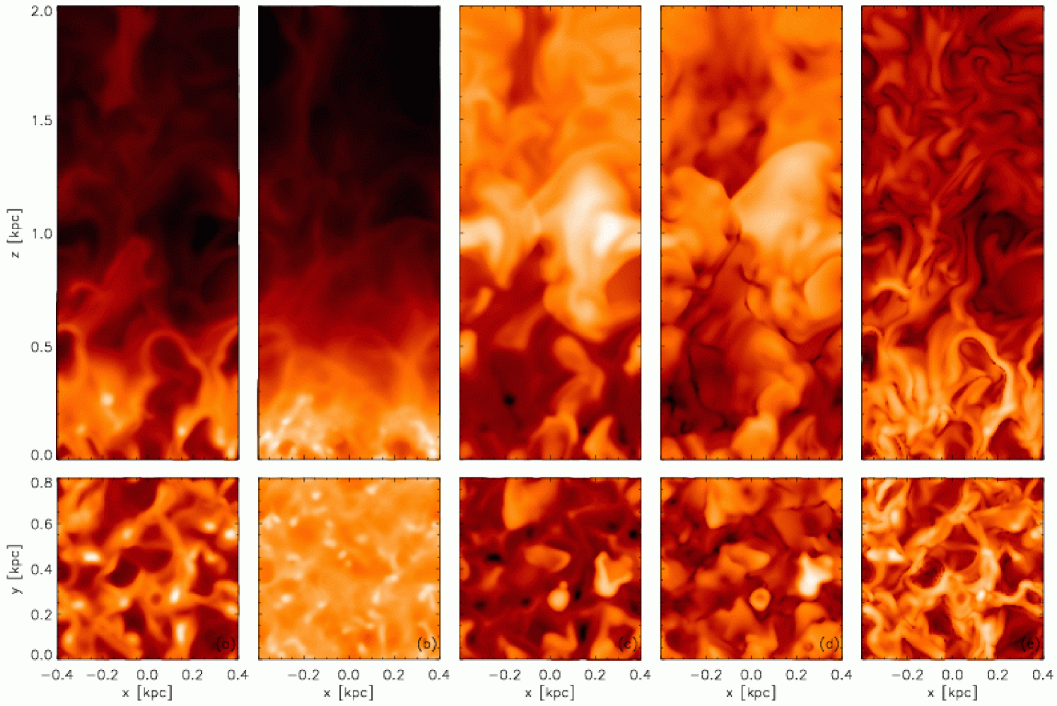
Figure 1: Vertical slices of the top half of our box (upper panels), and horizontal slices through the midplane (lower panels) after $t=112\,\rm Myr$. Quantities shown are: (a) number density $[\,\rm cm^{-3}]$, (b) column density $[\,\rm cm^{-2}]$, (c) temperature $[\,\rm K]$, (d) velocity dispersion $[\,\rm km\,s^{-1}]$, and (e) magnetic field strength $[\mu G]$. The logarithmic grey scales extend over ranges $[-4.82,1.10]$, $[17.34,21.55]$, $[2.06,7.20]$, $[-0.15,2.77]$, and $[-4.16,0.34]$ for the corresponding variables.

2.1 Supernova driving

We model supernova explosions as local injections of thermal energy resulting in turbulence at mildly supersonic Mach numbers. To assure convergence of the emerging supernova remnants numerical solutions with increasing spatial resolution $\Delta s$ have been tested against the analytical description by Cioffi, McKee & Bertschinger (1988). The results agree well and correspond to the findings reported in Mac Low et al. (2005).

SN-events are exponentially distributed in the vertical direction with scale heights of $325\,\rm\,pc$ for type-I and $90\,\rm\,pc$ for type-II SNe. For the models presented in this paper we use 3/4 the galactic frequencies which are $\sigma_{\rm I}=4\,\rm Myr^{-1}\,\rm kpc^{-2}$ respectively $\sigma_{\rm II}=30\,\rm Myr^{-1}\,\rm kpc^{-2}$. The associated explosion energies are $10^{51}$ and $1.14\!\times\!10^{51}\,\rm erg$ (Ferrière 2001).

Within our model we make an important distinction between type-I and type-II SNe. The latter are spatially clustered by the (artificial) constraint that the density at the explosion site must be above average (with respect to a horizontal slab) while the former are spatially uncorrelated (Korpi et al. 1999). We use this simple prescription as a proxy for a more self-consistent treatment of the clustering (de Avillez & Breitschwerdt 2005) and find a fraction of clustered events comparable to observations (Ferrière 2001). The reference simulation without SBs reveals that the general morphology is affected quite strongly by the clustering indicating the importance of this effect.

2.2 Radiative cooling and diffuse heating

	dom. $[\,\rm kpc]$	grid	SNe	cl.	q	$\beta_{\rm P}$
STD	$0.8,\pm$2.00	$96^{2}\!\times\!480$	I+II	y	0	2000
NCL	$0.8,\pm$2.00	$96^{2}\!\times\!480$	I+II	n	0	2000
SHR	$0.8,\pm$2.13	$96^{2}\!\times\!512$	I+II	y	-1	2000
SN2	$0.8,\pm$2.00	$96^{2}\!\times\!480$	II	y	0	2000
KIN	$0.8,\pm$2.00	$96^{2}\!\times\!480$	I+II	y	0	$\infty$

Table 1: Overview of conducted models. Clustering (’cl.’) applies to type-II SNe only. SN-rates are 3/4 the galactic values.

We treat the interstellar medium as an optically thin plasma and prescribe the coupling to the radiation field via a piecewise power law of the form: $\Lambda(T)=\Lambda_{i}\,T^{\beta_{i}}$, for $T_{i}\leq T<T_{i+1}$. The parameters used are essentially a combination of the cooling curves given by Sánchez-Salcedo, Vázquez-Semadeni & Gazol (2002) and Slyz et al. (2005), where the coefficients have been slightly modified to make the resulting curve continuous. In contrast to previous work by Korpi et al. (1999) we include the thermally unstable regime below $6102\,\rm K$ leading to the formation of a cold ISM phase. To numerically resolve the cooling instability we apply thermal conduction such that the Field length $\lambda_{\rm F}$ is covered by 4 grid cells (cf. Koyama & Inutsuka 2004). The various effects that contribute to the diffuse heating of the interstellar plasma are subsumed in a prescribed heating rate $\Gamma(z)=\Gamma_{0}\,e^{-z/h}$, with $h=300\,\rm\,pc$ as discussed in Joung & Mac Low (2006).

2.3 The initial model

Previous stratified models (Korpi et al. 1999; de Avillez & Breitschwerdt 2004; Joung & Mac Low 2006; Piontek & Ostriker 2007) all start from an isothermal initial state at a prescribed temperature. The main drawback of this is that the isothermal stratification is not in radiative equilibrium and the disk will instantaneously collapse until the dynamic pressure from SN- or MRI-turbulence will balance this process. To avoid this undesired behavior we propose a more sophisticated initial model where the vertical profiles of density and pressure are numerically integrated to be in combined hydrostatic and radiative equilibrium. The computed profiles are considerably flatter than the isothermal ones while the temperature varies by a factor of about five.

For our fiducial model we choose an initial midplane density $\rho_{0}$ corresponding to one particle per $\,\rm cm^{3}$ which results in an equilibrium pressure of $p_{0}/k_{B}=6000\,\rm K\,\rm cm^{-3}$. We use a mean molecular weight of $\bar{\mu}=0.6$ assuming a fully ionized plasma of cosmic abundance. For the current study the rotation rate is fixed at $\Omega=100\,\rm km\,s^{-1}\,\,\rm kpc^{-1}$. As in Brandenburg, Korpi & Mee (2007) we scale the dynamic viscosity coefficient with the density, i.e., we use a constant kinematic viscosity of $\nu=5\!\times\!10^{24}\,\,\rm cm^{2}s^{-1}$. To obtain a constant Prandtl number of ${\rm Pr}=4.2$ we apply the same scaling to the thermal conduction coefficient $\kappa$.

The magnetic Prandtl number ${\rm Pm}=\nu/\eta$ is thought to be very high for the ISM. With the limited dynamic range of our simulations we are, however, restricted to values close to unity. For practical purposes we choose ${\rm Pm}=2.5$ equivalent $\eta=2\!\times\!10^{24}\,\,\rm cm^{2}s^{-1}$ which is still two orders of magnitude smaller than the expected turbulent diffusivities.

The vertical boundary conditions are of the outflow type with the magnetic field extrapolated according to the solenoidal constraint. Due to the (sheared-) periodic boundary conditions in the x- and y-direction the vertical magnetic field is ideally conserved for any horizontal slab. This means that there are two distinct classes of models including or excluding vertical magnetic flux. For simplicity we focus on the latter case and start from an initially toroidal plus radial field with a pitch angle of $-6\degr$. The field is scaled with $\sqrt{p/p_{0}}$ to yield a constant plasma parameter $\beta_{\rm P}=2p/B^{2}\approx 2000$ throughout the disk. The resulting Alfvén velocity for the initial model is $0.3-0.6\,\rm km\,s^{-1}$ whereas the sound speed ranges from $10-20\,\rm km\,s^{-1}$. The particular choice of parameters for the conducted models is summarized in Table 1.

3 Numerical methods

For our computations we make use of the newly developed version 3 of the NIRVANA code (Ziegler 2004, 2005) which is a general purpose MHD fluid tool employing the technique of adaptive mesh refinement (AMR). For the simulations presented here this feature is, however, not being employed. We extended the standard shearingbox model to be compatible with the conservative numerical scheme and apply flux-matching at the sheared interfaces to improve the conservation properties (Gressel & Ziegler 2007).

3.1 Dynamo test fields

To find a closure for the mean field equations one strives to parameterize $\mathcal{E}=\overline{\mathbf{u}^{\prime}\!\times\!\mathbf{B}^{\prime}}$ with respect to averaged quantities. Here we adopt the standard description where $\mathcal{E}$ depends on the mean field and its gradients. When using spatial averages along horizontal slabs Brandenburg & Sokoloff (2002) showed that the resistivity tensor can be reduced and one yields:

$$\mathcal{E}_{i}=\alpha_{ij}\bar{B}_{j}-\tilde{\eta}_{ij}\varepsilon_{jkl}\partial_{k}\bar{B}_{l}\,,\quad i,j\in\left\{R,\phi\right\},k=z\,.$$ (1)

While the diagonal elements of ${\boldsymbol{\alpha}}$ quantify the dynamo process, its anti-symmetric off-diagonal elements constitute the vertical pumping effect described by the parameter $\gamma_{z}=0.5\,(\alpha_{\phi R}\!-\!\alpha_{R\phi})$. Similarly the diagonal elements of ${\tilde{\boldsymbol{\eta}}}$ are interpreted as turbulent resistivity $\eta_{t}$, while its off-diagonal components can lead to $\mathbf{\Omega\!\times\!J}$-type dynamo effects (Rüdiger & Hollerbach 2004). In total we have 4+4 unknowns that we wish to determine from equation (1).

To avoid complications with the inversion of this tensorial equation, we apply the test field approach proposed by Schrinner et al. (2005, 2007). The method has also recently been adopted to the shearingbox case by Brandenburg (2005). Earlier approaches (Brandenburg & Sokoloff 2002; Kowal et al. 2005) were based on least square fit methods. The major drawback with these was that in regions where $\bar{\mathbf{B}}$ or $\nabla\bar{\mathbf{B}}$ vanishes the inversion becomes singular. This can be circumvented by solving equation (1) for fixed test fields $\bar{\mathcal{B}}_{(\nu)}$ with simple, well behaved geometry and gradients. To obtain the related EMFs one has to evolve an extra (passive) induction equation for the associated fluctuations:

$$\partial_{t}\mathcal{B}^{\prime}_{(\nu)} = \nabla\times[\ \mathbf{u}^{\prime}\!\times\!\bar{\mathcal{B}}_{(\nu)}+(\bar{\mathbf{u}}\!+\!q\Omega x\hat{{\mathbf{y}}})\!\times\!\mathcal{B}^{\prime}_{(\nu)}$$

$$-\overline{\mathbf{u}^{\prime}\!\times\!\mathcal{B}^{\prime}}\!_{(\nu)}+\mathbf{u}^{\prime}\!\times\!\mathcal{B}^{\prime}_{(\nu)}-\eta\nabla\!\times\!\mathcal{B}^{\prime}_{(\nu)}\;]\,,$$

$$\nabla\!\cdot\!\mathcal{B}^{\prime}_{(\nu)} = 0\,.$$ (2)

We implemented these additional equations within NIRVANA employing the constrained transport paradigm to exactly satisfy the solenoidal constraint. The actual method uses up-winding to guarantee stability while second order in space is attained via piecewise linear reconstruction. For this we apply the same slope limiter as in the actual code. Our procedure is very similar to the methods described in Teyssier, Fromang & Dormy (2006).

For the particular choice of the four test fields $\bar{\mathcal{B}}_{(\nu)}$ we use the ones from Brandenburg (2005), i.e., the lowest Fourier modes in the vertical direction. For each of the test fields we compute the corresponding mean electromotive force

$$\bar{\mathcal{E}}^{(\nu)}=\overline{\mathbf{u}^{\prime}\!\times\!\mathcal{B}^{\prime}}\!_{(\nu)}\,.$$ (3)

The dynamo coefficients can then be computed via equation (1) to which the solution can be compactly written as

$$\left(\begin{array}[]{c}\alpha_{ij}\\ k_{1}\eta_{ij3}\end{array}\right)=\left(\begin{array}[]{cc}\,\,\cos(k_{1}\!z)&\sin(k_{1}\!z)\\ \!\!-\sin(k_{1}\!z)&\cos(k_{1}\!z)\end{array}\right)\left(\begin{array}[]{c}\bar{\mathcal{E}}_{i}^{(2j\!-\!2)}\\ \bar{\mathcal{E}}_{i}^{(2j\!-\!1)}\end{array}\right)\,,$$ (4)

with $i,j\in\{1,2\}$. In contrast to the least square fit method equation (4) can be directly computed for each $z$, yielding vertical profiles for the dynamo parameters.

4 Results and discussion

Since our vertical stratification is in radiative equilibrium, we do not observe an initial collapse of the disk. Turbulence builds up smoothly and after 100Myr reaches a quasi steady state. Fig. 1 shows vertical and horizontal slices through the simulation box at $t=112\,\rm Myr$. Most of the material is contained in cold clumps forming a $150-200\,\rm\,pc$ wide disk. Close to the midplane the network of clumps and filaments is permeated by strong shocks from the SNe which are continously creating hot cavities. Looking at the lower panels (a) and (e) of Fig. 1 one can see that for the region around the midplane there exists a significant correlation between the density and the magnetic field amplitude. The inferred slope of the correlation is somewhat steeper than the Chandrasekhar-Fermi value of $0.5$ but roughly consistent with $|B|\sim\rho^{2/3}$ as indicative of compressional amplification.

While single SNRs are largely confined to the midplane, super-bubbles break out of the central disk and drive moderate vertical flows. Their dense shells that are further compressed by shocks will form clouds that can efficiently cool and will in turn rain back into the gravitational potential thus forming what is termed the galactic fountain (Bregman 1980). The Mach number of the flow is mildly supersonic below $1\,\,\rm kpc$ and becomes subsonic for the outer parts.

If we turn off the SN-clustering the morphology changes quite drastically. Instead of well confined SBs we see more disrupted features and chimney-like structures that channel strong vertical outflows. The velocity dispersion in the hot phase is twice as high as in the clustered case. These differences demonstrate the importance of a proper modeling of clustered explosions.

4.1 Thermal distribution and velocity dispersions

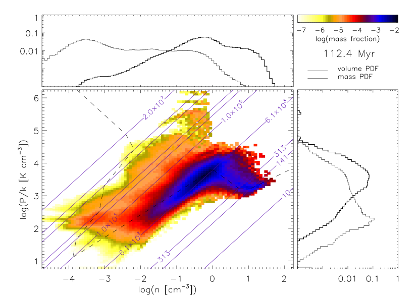
Figure 2: Phase space distribution of the SN-heated plasma. Adjacent plots show the mass- (thick) and volume- (thin line) distribution of density (upper panel) and pressure (right panel). We also plot isothermal contours (labeled in$\,\rm K$), and the equilibrium cooling curve (dashed).

In Fig. 2 we show the distribution of the SN-heated plasma as a function of density and thermal pressure at a time $t=112\,\rm Myr$. The two stable branches of the equilibrium curve are densely populated but there also exists a considerable amount of gas in the radiatively unstable regimes.

Averaged velocity dispersions for the ISM phases are $5\,\rm km\,s^{-1}$ (cold), $11\,\rm km\,s^{-1}$ (cool), $25\,\rm km\,s^{-1}$ (warm), and $40-60\,\rm km\,s^{-1}$ (hot). While the values for the latter are consistent with the findings of de Avillez & Breitschwerdt (2005), for the cold phases we fall short by a factor of two. We consider this a resolution issue but it might also be related to the different form of the driving. As a function of galactic height the time averaged rms-velocity rises steeply from its midplane value of $20\,\rm km\,s^{-1}$ to its peak value of $55\,\rm km\,s^{-1}$ which is reached at about $1\,\,\rm kpc$ and then falls off to about $30\,\rm km\,s^{-1}$ at $2\,\,\rm kpc$. Assuming that diamagnetic pumping follows the inverse gradient in turbulence intensity this implies an inward transport of magnetic flux for the central part of the disk.

4.2 Dynamo parameters

In Fig. 3 we plot the main $\alpha$- and $\eta$-coefficients for our standard run (mod. STD). To our knowledge this is the first time such profiles have been obtained from direct simulations of SN-turbulence. The corresponding vertically averaged amplitudes are listed in Table 2 – for comparison we also list the peak values from FER98 (where $\eta_{t}$ is distinguished into horizontal and vertical part). Dynamo numbers $C_{\alpha}=\alpha H/\eta_{t}$ and $C_{\Omega}=\Omega H^{2}/\eta_{t}$ are computed with $H=0.8\,\,\rm kpc$ and $\eta_{t}$ values from the inner part of the disk. In accordance with analytical estimations based on these numbers, the runs without shear are still sub-critical, i.e., no field-amplification is observed. The $\alpha^{2}\Omega$-dynamo, however, does exponentially grow at a time scale of $\sim 250\,\rm Myr$.

During the course of the present simulations we do not yet reach the equipartition field strength. This implies that the values for the dynamo parameters (as well as the pitch angle) are representative of the unquenched regime.

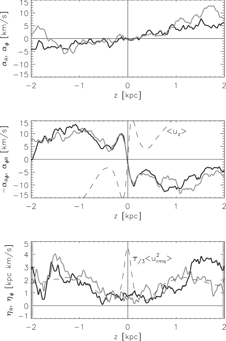
Figure 3: Dynamo $\alpha$- and $\eta$-coefficients for the STD model. Quantities indicated by the ordinate labels are plotted in dark ($\alpha_{RR},\dots$) respectively light ($\alpha_{\phi\phi},\dots$) colors. Shaded areas indicate the rms-fluctuation when applying the method to 4 temporal sub-intervals.

Our values are still affected by fluctuations and a longer time-base is needed for a more accurate determination. However, we find some interesting trends in the data at hand: The antisymmetric part $\gamma_{z}$ of the $\alpha$-tensor is negative (positive) in the northern (southern) hemisphere, i.e., pumping is directed inward. This is contrary to the predictions by Ferrière for the case of non-interacting SNRs. In our simulations the inward pumping is opposed by an outward advection of the field with the mean flow. As can be seen from the middle panel of Fig. 3 both terms have about the same magnitude for $z<1\,\,\rm kpc$ while in the corona the wind is dominating. The balance in the inner region could be seen as an indication that the effects of turbulent pumping and advection are naturally linked. In consequence vertical transport processes might be of lesser importance than formerly believed.

The importance of modeling spatially coherent SBs can be seen from comparing the first two rows of Table 2. In the case without clustered SNe (mod. NCL) we observe strong vertical streaming motions reflected in high values for $\gamma_{z}$ and $\bar{u}_{z}$. Also the turbulent diffusivity is high in the disk midplane which is not the case for the other runs where $\eta_{t}$ increases with galactic height. From the model with type-II SNe only (mod. SN2) one can learn that the turbulent diffusivity predominantly arises from the more broadly distributed type-I SNe – despite their lower rate by a factor of eight. The overall level of turbulent diffusion is about $3$–$6\!\times\!10^{26}\,\,\rm cm^{2}s^{-1}$. The off-diagonal components of the $\eta$-tensor are somewhat smaller and cannot yet be determined accurately. Following Jin (1996) we crudely estimate that the measured amount of diffusion suffices to damp short wavelength MRI-modes for reasonably high $\beta_{\rm P}$ – a definite conclusion, however, requires further investigations by means of combined direct simulations.

By comparing $\alpha_{\phi\phi}$ with the SOCA results by Rüdiger & Kichatinov (1993) we can estimate the coherence time $\tau$ and the Coriolis number $\Omega^{*}=2\tau\Omega$ of our turbulent flow. We find a value of $\tau\approx 3.6\,\rm Myr$ which is about a factor of three smaller than commonly assumed. The even lower value for our model NCL indicates that a higher coherence time might be achieved by a more realistic prescription for the modeling of SBs. In general the obtained profiles are consistent with their SOCA counterparts. Our obtained value for $\hat{\gamma}=|\alpha_{\phi R}|/|\alpha_{\phi\phi}|$ agrees with the SOCA value of $\hat{\gamma}\approx 2.5$ in Rüdiger & Hollerbach (2004) and is smaller than the value of $\hat{\gamma}\approx 6$ in FER98.

In the lower panel of Fig. 3 we overplot the scalar expression for the turbulent diffusivity which matches the profiles obtained from the simulations. The peak of the velocity dispersion close to the midplane is an artifact due to the static distribution of the SNe resulting in a disruption of the central disk. This issue has meanwhile been resolved.

	$|\alpha_{RR}|$	$|\alpha_{\phi\phi}|$	$|\gamma_{z}|$	$\hat{\gamma}$	$\eta_{t}$		$\tau$	$\Omega^{*}$	$C_{\alpha}$
	$[\,\rm km\,s^{-1}]$	$[\,\rm km\,s^{-1}]$	$[\,\rm km\,s^{-1}]$		$[\,\rm kpc\,\rm km\,s^{-1}]$		$[\,\rm Myr]$
STD	3.1	3.8	7.8	2.1	0.9	2.7	3.6	0.7	3.3
NCL	7.3	4.3	24.7	5.9	2.4	2.2	2.8	0.6	1.4
SN2	0.8	0.8	1.8	2.5	0.6	1.0	3.6	0.7	1.2
KIN	3.2	2.0	8.3	4.1	0.6	1.2	3.4	0.7	2.6
FER98	6.0	2.6	16.0	6.2	3 – 18		–	–	0.5

Table 2: Mean values of extracted parameters averaged over $\approx 150\,\rm Myr$. Values for $\eta_{t}$ apply to the inner ($|z|\leq 0.8\,\,\rm kpc$) respectively outer region of the disk. Coherence time $\tau$ and Coriolis number $\Omega^{*}$ are estimated from a comparison with SOCA-profiles for $\alpha_{\phi\phi}$. The coefficients could not be obtained for model SHR.

4.3 Pitch angles

In our models without shear we observe pitch angles ranging from $+10\degr$ in the far outer regions to $-45\degr$ near the midplane. This is hardly surprising since also the radial and azimuthal dynamo effects are found to be of equal strength in this case. If we include galactic shear with $q=-1$, pitch angles become solely negative reaching values up to $-30\degr$ as consistent with observations. The minimum of $-10\degr$ is found at the midplane. In comparison, Hanasz et al. (2006) in their simulations of a cosmic ray driven galactic dynamo find the azimuthal field to be dominating by a factor of ten which corresponds to pitch angles of only $\sim 5\degr$.

5 Summary

We have performed resistive MHD simulations of the differentially rotating, stratified local interstellar medium. By integrating a radiatively stable initial stratification we were able to avoid the disk collapse occurring in previous isothermal models. We have further demonstrated that SNe can indeed produce an $\alpha$-effect that is not dominated by vertical pumping. Our key findings are as follows:

• The turbulent velocity dispersion in our box increases with galactic height, i.e., the diamagnetic pumping is directed inward.

• We observe a mean vertical outflow of the same magnitude as the turbulent pumping. In consequence this drastically reduces the effective vertical transport of the mean magnetic field.

• The ratio $\hat{\gamma}$ of vertical pumping over the $\alpha$-effect is diminished if type-II SNe are modeled as clustered events.

• The radial pitch angles found in our simulations are consistent with observations and suggest an $\alpha^{2}\Omega$-dynamo.