Cobweb posets - Recent Results

A. Krzysztof Kwaśniewski (*) ,M. Dziemiańczuk (**)

(*) the Dissident - relegated by Białystok University authorities
from the Institute of Informatics to Faculty of Physics
ul. Lipowa 41, 15 424 Białystok, Poland
e-mail: kwandr@gmail.com
(**) Former Student in the Institute of Computer Science, Białystok University; then moved to:
Institute of Informatics, University of Gdańsk, Poland;
e-mail: mdziemianczuk@gmail.com

SUMMARY

Cobweb posets uniquely represented by directed acyclic graphs are such a generalization of the Fibonacci tree that allows joint combinatorial interpretation for all of them under admissibility condition. This interpretation was derived in the source papers ([6,7] and references therein to the first author).[7,6,8] include natural enquires to be reported on here. The purpose of this presentation is to report on the progress in solving computational problems which are quite easily formulated for the new class of directed acyclic graphs interpreted as Hasse diagrams. The problems posed there and not yet all solved completely are of crucial importance for the vast class of new partially ordered sets with joint combinatorial interpretation. These so called cobweb posets - are relatives of Fibonacci tree and are labeled by specific number sequences - natural numbers sequence and Fibonacci sequence included. One presents here also a join combinatorial interpretation of those posets‘ $F$-nomial coefficients which are computed with the so called cobweb admissible sequences. Cobweb posets and their natural subposets are graded posets. They are vertex partitioned into such antichains $\Phi_{n}$ (where $n$ is a nonnegative integer) that for each $\Phi_{n}$, all of the elements covering $x$ are in $\Phi_{n+1}$ and all the elements covered by $x$ are in $\Phi_{n}$. We shall call the $\Phi_{n}$ the $n-th$- level. The cobweb posets might be identified with a chain of di-bicliques i.e. by definition - a chain of complete bipartite one direction digraphs [6]. Any chain of relations is therefore obtainable from the cobweb poset chain of complete relations via deleting arcs in di-bicliques of the complete relations chain. In particular we response to one of those problems [1]. This is a tiling problem. Our information on tiling problem refers on proofs of tiling’s existence for some cobweb-admissible sequences as in [1]. There the second author shows that not all cobwebs admit tiling as defined below and provides examples of cobwebs admitting tiling.

Key Words: acyclic digraphs, tilings, special number sequences, binomial-like coefficients.

AMS Classification Numbers: 06A07 ,05C70,05C75, 11B39.

Presented at Gian-Carlo Polish Seminar:

http://ii.uwb.edu.pl/akk/sem/sem_rota.htm

published: Adv. Stud. Contemp. Math. vol. 16 (2) April (2008):197-218.

1 Introduction [6]

A directed acyclic graph, also called DAG, is a directed graph with no directed cycles. DAGs considered as a generalization of trees have a lot of applications in computer science, bioinformatics, physics and many natural activities of humanity and nature. Here we introduce specific DAGs as generalization of trees being inspired by algorithm of the Fibonacci tree growth. For any given natural numbers valued sequence the graded (layered) cobweb posets‘ DAGs are equivalently representations of a chain of binary relations. Every relation of the cobweb poset chain is biunivocally represented by the uniquely designated complete bipartite digraph-a digraph which is a di-biclique designated by the very given sequence. The cobweb poset is then to be identified with a chain of di-bicliques i.e. by definition - a chain of complete bipartite one direction digraphs. Any chain of relations is therefore obtainable from the cobweb poset chain of complete relations via deleting arcs (arrows) in di-bicliques.
Let us underline it again : any chain of relations is obtainable from the cobweb poset chain of complete relations via deleting arcs in di-bicliques of the complete relations chain. For that to see note that any relation $R_{k}$ as a subset of $A_{k}\times A_{k+1}$ is represented by a one-direction bipartite digraph $D_{k}$. A ”complete relation” $C_{k}$ by definition is identified with its one direction di-biclique graph $d-B_{k}$ Any $R_{k}$ is a subset of $C_{k}$. Correspondingly one direction digraph $D_{k}$ is a subgraph of an one direction digraph of $d-B_{k}$.
The one direction digraph of $d-B_{k}$ is called since now on the di-biclique i.e. by definition - a complete bipartite one direction digraph. Another words: cobweb poset defining di-bicliques are links of a complete relations’ chain [6].

Because of that the cobweb posets in the family of all chains of relations unavoidably is of principle importance being the most overwhelming case of relations’ infinite chains or their finite parts (i.e. vide - subposets).

The intuitively transparent names used above (a chain of di-cliques etc.) are to be the names of defined objects in what follows. These are natural correspondents to their undirected graphs relatives as we can view a directed graph as an undirected graph with arrowheads added.

The purpose of this report is to inform several questions intriguing on their own apart from being fundamental for a new class of DAGs introduced below. Specifically this concerns problems which arise naturally in connection with a new join combinatorial interpretation of all classical $F-binomial$ coefficients - Newton binomial, Gaussian $q$-binomial and Fibonomial coefficients included. This report is based on [6-7] from which definitions and description of these new DAG’s are quoted for the sake of self consistency and last results are taken from [1]. Applications of new cobweb posets‘ originated Whitney numbers from [8] such as extended Stirling or Bell numbers are expected to be of at least such a significance in applications to linear algebra of formal series as Stirling numbers, Bell numbers or their $q$-extended correspondent already are in the so called coherent states physics [9,10] (see [13] for abundant references on this subject and other applications such as in [11,12]).

The problem to be the next. As cobweb subposets $P_{n}$ are vertex partitioned into antichains $\Phi_{r}$ for $r=0,1,...,n$ which we call levels - a question of canonical importance arises. Let $\left\{P_{n}\right\}_{n\geq 0}$ be the sequence of finite cobweb subposets (see- below). What is the form and properties of $\left\{P_{n}\right\}_{n\geq 0}$’s characteristic polynomials $\left\{\rho_{n}(\lambda)\right\}_{n\geq 0}$ [15,17]? For example - are these related to umbra polynomials? What are recurrence relations defining the $\left\{\rho_{n}(\lambda)\right\}_{n\geq 0}$ family ? This is being now under investigation with a progress to be announced soon by Ewa Krot-Sieniawska [4,5] - the member of our Rota Polish Seminar Group. The recent papers on DAGs related to this article and its clue references [6,7,8] apart from [1] are [4] and [14].

Computation and Characterizing Problems.

In the next section we define cobweb posets. Their examples are given [6-8,1]. A join combinatorial interpretation of cobweb posets‘ characteristic binomial-like coefficients is provided too following the source papers of the first author. This simultaneously means that we have join combinatorial interpretation of fibonomial coefficients and all incidence coefficients of reduced incidence algebras of full binomial type [16].

In [6,7] the first author had formulated three problems: characterization and/or computation of cobweb admissible sequences Problem 1, cobweb layers partition characterization and/or computation Problem 2 and the GCD-morphic sequences characterizations and/or computation Problem 3 all three interesting on their own. Here we report more on one of those problems [1]. This is a tiling problem. Our information on tiling problem refers to proofs of tiling’s existence for some cobweb-admissible sequences as in [1]. There the second author shows that not all cobwebs admit tiling as defined below and provides examples with proofs of families of cobweb posets which admit tiling.

2 Cobweb posets as complete bipartite digraph sequences and combinatorial interpretation [6]

Cobweb posets as complete bipartite digraph sequences.

Cobweb posets and their natural subposets $P_{n}$ are graded posets. They are vertex partitioned into antichains $\Phi_{k}$ for $k=0,1,...,r,...$ (where $r$ is a nonnegative integer) such that for each $\Phi_{r}$, all of the elements covering $x$ are in $\Phi_{r+1}$ and all the elements covered by $x$ are in $\Phi_{r}$. We shall call the $\Phi_{n}$ the $n-th$-level. $P_{n}$ is then $(n+1)$ level ranked poset. We are now in a position to observe that the cobweb posets may be identified with a chain of di-bicliques i.e. by definition - a chain of complete bipartite one direction digraphs. This is outstanding property as then any chain of relations is obtainable from the corresponding cobweb poset chain of complete relations just by deleting arcs in di-bicliques of this complete relations chain. Indeed. For any given natural numbers valued sequence the graded (layered) cobweb posets‘ DAGs are equivalently representations of a chain of binary relations. Every relation of the cobweb poset chain is bi-univocally represented by the uniquely designated complete bipartite digraph - a digraph which is a di-biclique designated by the very given sequence. The cobweb poset may be therefore identified with a chain of di-bicliques i.e. by definition - a chain of complete bipartite one direction digraphs. Say it again, any chain of relations is obtainable from the cobweb poset chain of complete relations via deleting arcs (arrows) in chains‘ di-bicliques elements.

The above intuitively transparent names (a chain of di-cliques etc.) are the names of the below defined objects. These objects are natural correspondents of their undirected graphs relatives as we can view a directed graph as an undirected graph with arrowheads added. Let us start with primary notions remembering that any cobweb subposet $P_{k}$ is a DAG of course.

A bipartite digraph is a digraph whose vertices can be divided into two disjoint sets $V_{1}$ and $V_{2}$ such that every arc connects a vertex in $V_{1}$ and a vertex in $V_{2}$. Note that there is no arc between two vertices in the same independent set $V_{1}$ or $V_{2}$. No two nodes of the same partition set are adjacent.

A one direction bipartite digraph is a bipartite digraph such that every arc originates at a node in $V_{1}$ and terminates at a node in $V_{2}$. The extension of ”being one direction” to $k$-partite digraphs is automatic. Note that there is no arc between two vertices in the same set. Intuitively - one may color the nodes of a bipartite digraph black and blue such that no arc exists between like colors.

A $k$-partite not necessarily one direction digraph $D$ is obtained from a $k$-partite undirected $k$-partite graph $G$ by replacing every edge ${xy}$ of $G$ with the arc $\left\langle xy\right\rangle$, arc $\left\langle yx\right\rangle$ or both $\left\langle xy\right\rangle$ and $\left\langle yx\right\rangle$. The partite sets of $D$ are the partite sets of $G$.

Definition 1

. A simple directed graph $G=(V,E)$ is called bipartite if there exists a partition $V=V_{1}+V_{2}$ of the vertex set $V$ so that every edge (arc) in E is incident with $v_{1}$ and $v_{2}$ for some $v_{1}$ in $V_{1}$ and $v_{2}$ in $V_{2}$. It is complete if any node from $V_{1}$ is adjacent to all nodes of $V_{2}$.

We shall denote our special case biparte one direction digraphs as follows $G=(V_{1}+V_{2},E)\equiv L_{{F_{k}},F_{k+1}}$ to inform that the partition has parts $V_{1}$ and $V_{2}$ where $\left|V_{1}\right|=F_{k}$ and $\left|V_{2}\right|=F_{k+1}.$

Notation. The special $k$ - partite $\equiv$ $k$ - level one direction digraphs considered here shall be denoted by the corresponding symbol $L_{p,q,...,r}$. The complete $k$ -partite $\equiv$ $k$ -level one direction complete digraph is coded $K_{p,q,...,r}$ as in the non directed case (with no place for confusion because only one direction digraphs are to be considered in what follows). $L_{{F_{k}},F_{k+1},...,F_{n}}\equiv\langle\Phi_{k}\rightarrow\Phi_{n}\rangle$ denotes $(n-k+1)$ - partite one direction digraph $\equiv(n-k+1)$ - level one direction digraph $n\geq k$ whose partition has ( antichains from $\Pi$) the parts $\Phi_{k},\Phi_{k+1},...,\Phi_{n},\;\left|\Phi_{k}\right|=F_{k},\left|\Phi_{k+1}\right|=F_{k+1},,\left|\Phi_{n}\right|=F_{n}.$ Any cobweb one-layer $\langle\Phi_{k}\rightarrow\Phi_{k+1}\rangle,\quad k<n,\quad k,n\in N\cup\{0\}\equiv Z_{\geq}$ is a complete bipartite one direction digraph $L_{{F_{i}},F_{i+1}}=K_{{F_{i}},F_{i+1}}$ i.e. by definition it is the di-biclique. The cobweb one-layer vertices constitute bipartite set $V(\langle\Phi_{k}\rightarrow\Phi_{k+1}\rangle)=\Phi_{k}+\Phi_{k+1}$ while edges are all those arcs incident with the two antichains nodes in the poset $\Pi$ graph representation.
Any cobweb subposet $P_{n}\equiv\langle\Phi_{0}\rightarrow\Phi_{n}\rangle\equiv L_{F_{0},F_{1},...,F_{n}},n\geq 0$ is a $(n+1)$-partite = $(n+1)$-level one direction digraph. We shall keep on calling a complete bipartite one direction digraph a di-biclique because it is a special kind of bipartite one direction digraph, whose every vertex of the first set is connected by an arc originated in this very node to every vertex of the second set of the given bi-partition. Any cobweb layer $\langle\Phi_{k}\rightarrow\Phi_{n}\rangle,\quad k\leq n,\quad k,n\in N\cup\{0\}\equiv Z_{\geq}$ is a one direction the $(n-k+1)$-partite $\equiv$ $(n-k+1)$-level one direction DAG $L_{{F_{k}},F_{k+1},...,F_{n}}$ with an additional defining property: it is a chain of di-bicliques for $k<n$. Since now on we shall identify both:

$$\langle\Phi_{k}\rightarrow\Phi_{n}\rangle=L_{{F_{k}},F_{k+1},...,F_{n}}.$$

Note: $P_{n}$ $\equiv$ $\langle\Phi_{0}\rightarrow\Phi_{n}\rangle=L_{{F_{0}},F_{k+1},...,F_{n}},\;n\geq 0$ and $\langle\Phi_{k}\rightarrow\Phi_{n}\rangle\neg=K_{{F_{k}},F_{k+1},...,F_{n}}$ for $n>k+1.$

Observation 1 (6)

$$\left|E(\langle\Phi_{k}\rightarrow\Phi_{k+m}\rangle)\right|={\sum}^{m-1}_{i=0}F_{k+i}F_{k+i+1},$$

where $E(G)$ denotes the set of edges of a graph $G$ (arcs of a digraph $G$).

The following property $(*)$

$$(*)\ \ \ \langle\Phi_{k}\rightarrow\Phi_{k+1}\rangle\equiv L_{{F_{k}},F_{k+1}}=K_{{F_{k}},F_{k+1}},\ \ k=0,1,2,...$$

i.e. $L_{{F_{k}},F_{k+1}}$ is a di-biclique for $k=0,1,2,...$ , might be considered the definition of $F_{0}$ rooted $F$-cobweb graph $\Pi$ or in short $P$ if $F$-sequence has been established. The cobweb poset $\Pi$ is being thus identified with a chain of di-bicliques. The usual convention is to choose $F_{0}=1.$ One may relax this constrain, of course.

Thus any cobweb one-layer $\langle\Phi_{k}\rightarrow\Phi_{k+1}\rangle$ is a complete one direction bipartite digraph i.e. a di-biclique. This is how the definition of the $F$-cobweb graph $\Pi(F)$ or in short $P$ - has emerged.

For infinite cobweb poset $\Pi$ with the set of vertices $P=V(\Pi)$ one has an obvious $\delta(G)=2$ domatic vertex partition of this $F$-cobweb poset.

Definition 2

. A subset $D$ of the vertex set $V(G)$ of a digraph $G$ is called dominating in $G$, if each vertex of $G$ either is in $D$, or is adjacent to a vertex of $D$. Adjacent means that there exists an originating or terminating arc in between the two- any node from $G$ outside $D$ and a node from $D$.

Definition 3

. A domatic partition of $V$ is a partition of $V$ into dominating sets, and the number of these dominating sets is called the size of such a partition. The domatic number $\delta(G)$ is the maximum size of a domatic partition.

An infinite cobweb poset $\Pi$ with the set of vertices $P=V(\Pi)$ has the $\delta(\Pi)=2$ domatic vertex partition, namely a $mod\ 2$ - partition.

$V=V_{0}\cup V_{1}$ where $V_{0}=\bigcup_{k=2s+1}\Phi_{k},\ s=0,1,2,...$ - (”black levels”); and $V_{1}=\bigcup_{k=2s}\Phi_{k},\ s=0,1,2,...$ - (”blue levels”).

Note: Natural $mod\ n$ partitions of the cobweb poset‘s set of vertices $V(\Pi)=P$ ($n$ colours), $P=V_{0}\cup V_{1}\cup V_{2}\cup...\cup V_{n-1}$ , $V_{i}=\bigcup_{k=2s+i},s=0,1,2,...,i\in Z_{n}={0,1,...,n-1}$ for $n>2$ are not domatic.

Cobweb one-layer or more than one-layer subposets $\langle\Phi_{k}\rightarrow\Phi_{k+m}\rangle\equiv L_{{F_{k}},F_{k+1}}=K_{{F_{k}},F_{k+1}},\ \ k=0,1,2,...$ have also correspondent, obvious the $\delta(G)=2$ domatic partitions for $m>0.$

Combinatorial interpretation [7,19,24,25].

2.1. $F-binomial$ coefficients. The source papers are [9-13] from which indispensable definitions and notation are taken for granted including Kwaśniewski [9,10] upside - down notation $n_{F}\equiv F_{n}$ being used for dipper than mnemonic reasons - as it the case with widespread: a] Gaussian numbers $n_{q}$ in finite geometries and the so called ”quantum groups” ([8,9]) or b] their $p,q$ cognates $n_{p,q}=\sum_{j=0}^{n-1}{p^{n-j-1}q^{j}}$ , $n_{q}=n_{1,q}$ .

Given any sequence $\{F_{n}\}_{n\geq 0}$ of nonzero reals ($F_{0}=0$ being sometimes acceptable as $0!=F_{0}!=1.$) one defines its corresponding binomial-like $F-nomial$ coefficients as in Ward‘s Calculus of sequences [18] as follows.

Definition 4

.$(n_{F}\equiv F_{n}\neq 0,\quad n>0)$

$$\left(\begin{array}[]{c}n\\ k\end{array}\right)_{F}=\frac{F_{n}!}{F_{k}!F_{n-k}!}\equiv\frac{n_{F}^{\underline{k}}}{k_{F}!},\quad\quad n_{F}!\equiv n_{F}(n-1)_{F}(n-2)_{F}(n-3)_{F}\ldots 2_{F}1_{F};$$

$$0_{F}!=1;\quad n_{F}^{\underline{k}}=n_{F}(n-1)_{F}\ldots(n-k+1)_{F}.$$

We have made above an analogy driven identifications in the spirit of Ward‘s Calculus of sequences [18]]. Identification $n_{F}\equiv F_{n}$ is the notation used in extended Fibonomial Calculus case [9-13,4] being also there inspiring as $n_{F}$ mimics $n_{q}$ established notation for Gaussian integers exploited in much elaborated family of various applications including quantum physics (see [9,10,13] and references therein).

The crucial and elementary observation now is that an eventual cobweb poset or any combinatorial interpretation of $F$-binomial coefficients makes sense not for arbitrary $F$ sequences as $F-binomial$ coefficients should be nonnegative integers (hybrid sets are not considered here).

Definition 5

.[7,6,19,24,25] A natural numbers‘ valued sequence $F=\{n_{F}\}_{n\geq 0}$, $F_{0}=1$ is called cobweb-admissible iff

$$\left(\begin{array}[]{c}n\\ k\end{array}\right)_{F}\in N_{0}\quad for\quad k,n\in N_{0}.$$

$F_{0}=0$ being sometimes acceptable as $0_{F}!\equiv F_{0}!=1.$

Incidence coefficients of any reduced incidence algebra of full binomial type [16] immensely important for computer science are computed exactly with their correspondent cobweb-admissible sequences. These include binomial (Newton) or $q$- binomial (Gauss) coefficients. For other $F$-binomial coefficients - computed with cobweb admissible sequences - see in what follows after Observation 3.

Problem 1. Find effective characterizations and/or an algorithm to produce the cobweb admissible sequences i.e. find all examples. [6,7,19]

Very recently the second author have proved (a note in preparation) that the following is true.

Theorem 1 (Dziemiańczuk)

Any cobweb-admissible sequence $F$ is at the point product [1] of primary cobweb-admissible sequences $P(p)$.

Right from the definition of $P$ via its Hasse diagram pictures in [6-8] the important observations follow which lead to a specific, new joint combinatorial interpretation of cobweb poset‘s characteristic binomial-like coefficients [6-8].

Observation 2 (6,7,19,24,25)

The number of maximal chains starting from The Root (level $0_{F}$) to reach any point at the $n-th$ level with $n_{F}$ vertices is equal to $n_{F}!$.

Observation 3

, $(k>0)$ [6,7,19,24,25] The number of all maximal chains in-between $(k+1)-th$ level $\Phi_{k+1}$ and the $n-th$ level $\Phi_{n}$ with $n_{F}$ vertices is equal to $n_{F}^{\underline{m}}$,  where $m+k=n.$

Indeed. Denote the number of ways to get along maximal chains from any fixed point (the leftist for example) in $\Phi_{k}$ to any vertex in $\Phi_{n},n>k$ with the symbol

$$[\Phi_{k}\rightarrow\Phi_{n}]$$

then obviously we have ( $[\Phi_{n}\rightarrow\Phi_{n}]\equiv 1)$:

$$[\Phi_{0}\rightarrow\Phi_{n}]=n_{F}!$$

and

$$[\Phi_{0}\rightarrow\Phi_{k}]\times[\Phi_{k}\rightarrow\Phi_{n}]=[\Phi_{0}\rightarrow\Phi_{n}].$$

For the purpose of a new joint combinatorial interpretation of $F-sequence-nomial$ coefficients (F-nomial - in short) let us consider all finite ”max-disjoint” sub-posets rooted at the $k-th$ level at any fixed vertex $\langle r,k\rangle,1\leq r\leq k_{F}$ and ending at corresponding number of vertices at the $n-th$ level ($n=k+m$) where the max-disjoint sub-posets are defined below.

Definition 6

. [6,7,19,24,25] Two posets are said to be max-disjoint if considered as sets of maximal chains they are disjoint i.e. they have no maximal chain in common. An equipotent copy of $P_{m}$ [‘equip-copy’] is defined as such a maximal chains family equinumerous with $P_{m}$ set of maximal chains that the it constitutes a sub-poset with one minimal element.

We shall proceed with deliberate notation coincidence anticipating coming observation.

Definition 7

. Let us denote the number of all mutually max-disjoint equip-copies of $P_{m}$ rooted at any fixed vertex $\langle j,k\rangle,1\leq j\leq k_{F}$ of $k-th$ level with the symbol

$$\left(\begin{array}[]{c}n\\ k\end{array}\right)_{F}.$$

One uses here the customary convention: $\left(\begin{array}[]{c}0\\ 0\end{array}\right)_{F}=1$ and $\left(\begin{array}[]{c}n\\ n\end{array}\right)_{F}=1.$

Compare the above with the Definition 4 and the Definition 10.

The number of ways to reach an upper level from a lower one along any of maximal chains i.e. the number of all maximal chains from the level $\Phi_{k+1}$ to the level $\Phi_{n},\quad k>n$ is equal to

$$[\Phi_{k}\rightarrow\Phi_{n}]=n_{F}^{\underline{m}}.$$

Therefore we have

(1) $$\left(\begin{array}[]{c}n\\ k\end{array}\right)_{F}\times[\Phi_{0}\rightarrow\Phi_{m}]=[\Phi_{k}\rightarrow\Phi_{n}]=n_{F}^{\underline{m}}$$

where $[\Phi_{0}\rightarrow\Phi_{m}]=m_{F}!$ counts the number of maximal chains in any equip-copy of $P_{m}$. With this in mind we see that the following holds [6,7,19,24,25].

Observation 4

Let ${n,k}\geq 0$. Let $n=k+m$. Let $F$ be any cobweb admissible sequence. Then the number of mutually max-disjoint equip-copies i.e. sub-posets equipotent to $P_{m}$ , rooted at the same fixed vertex of $k-th$ level and ending at the n-th level is equal to

$$\frac{n_{F}^{\underline{m}}}{m_{F}!}=\left(\begin{array}[]{c}n\\ m\end{array}\right)_{F}$$

$$=\left(\begin{array}[]{c}n\\ k\end{array}\right)_{F}=\frac{n_{F}^{\underline{k}}}{k_{F}!}.$$

The immediate natural question now is

$$\Big{\{}{{\eta}\atop{\kappa}}\Big{\}}_{const}=?$$

i.e. the number of partitions with block sizes all equal to const = ?

where here $const=\lambda=m_{F}!$ and

$$\eta=n_{F}^{\underline{m}},\ \ \kappa=\left(\begin{array}[]{c}n\\ k\end{array}\right)_{F}$$

The const indicates that this is the number of set partitions with block sizes all equal to const and we use Knuth notation $\Big{\{}{{\eta}\atop{\kappa}}\Big{\}}$ for Stirling numbers of the second kind.

From the formula (59) in [2] one infers the Pascal-like matrix answer to the question above.

$$\Big{\{}{\eta\atop\kappa}\Big{\}}_{\lambda}=\delta_{\eta,\kappa\lambda}\frac{\eta!}{\kappa!\lambda!^{\kappa}}.$$

This gives us the rough upper bound for the number of tilings (see [6] for Pascal-like triangles) as we arrive now to the following intrinsically related problem.

The partition or tiling Problem 2. Suppose now that $F$ is a cobweb admissible sequence. Let us introduce

$$\sigma P_{m}=C_{m}[F;\sigma<F_{1},F_{2},...,F_{m}>]$$

the equipotent sub-poset obtained from $P_{m}$ with help of a permutation $\sigma$ of the sequence $<F_{1},F_{2},...,F_{m}>$ encoding $m$ layers of $P_{m}$ thus obtaining the equinumerous sub-poset $\sigma P_{m}$ with the sequence $\sigma<F_{1},F_{2},...,F_{m}>$ encoding now $m$ layers of $\sigma P_{m}$. Then $P_{m}=C_{m}[F;<F_{1},F_{2},...,F_{m}>].$ Consider the layer $\langle\Phi_{k}\rightarrow\Phi_{n}\rangle,\quad k<n,\quad k,n\in N$ partition into the equal size blocks which are here max-disjoint equi-copies of $P_{m},m=n-k+1$. The question then arises whether and under which conditions the layer may be partitioned with help of max-disjoint blocks of the form $\sigma P_{m}$. And how to visualize this phenomenon? It seems to be the question of computer art, too. At first - we already know that an answer to the main question of such tilings existence - for some sequences $F$ -is in affirmative. Whether is it so for all cobweb admissible sequences -we do not know by now. Some computer experiments done by student Maciej Dziemiańczuk [1] are encouraging. More than that. The second author in [1] proves tiling’s existence for some cobweb-admissible sequences including natural and Fibonacci numbers sequences. He shows also that not all $F$ - designated cobweb posets do admit tiling as defined above. However problems: ”how many?” is opened. Let us recapitulate and report on results obtained in [1].

3 Cobweb posets tiling problem

Let us recall that cobweb poset in its original form [6,7] is defined as a partially ordered graded infinite poset $\Pi=\langle P,\leq\rangle$, designated uniquely by any sequence of nonnegative integers $F=\{n_{F}\}_{n\geq 0}$ and it is represented as a directed acyclic graph (DAG) in the graphical display of its Hasse diagram. $P$ in $\langle P,\leq\rangle$ stays for set of vertices while $\leq$ denotes partially ordered relation. See Fig. 1 and note (quotation from [7,6]):

One refers to $\Phi_{s}$ as to the set of vertices at the $s$-th level. The population of the $k$-th level (”generation”) counts $k_{F}$ different member vertices for $k>0$ and one for $k=0$. Here down (Fig. 1) a disposal of vertices on $\Phi_{k}$ levels is visualized for the case of Fibonacci sequence. $F_{0}=0$ corresponds to the empty root $\{\emptyset\}$.

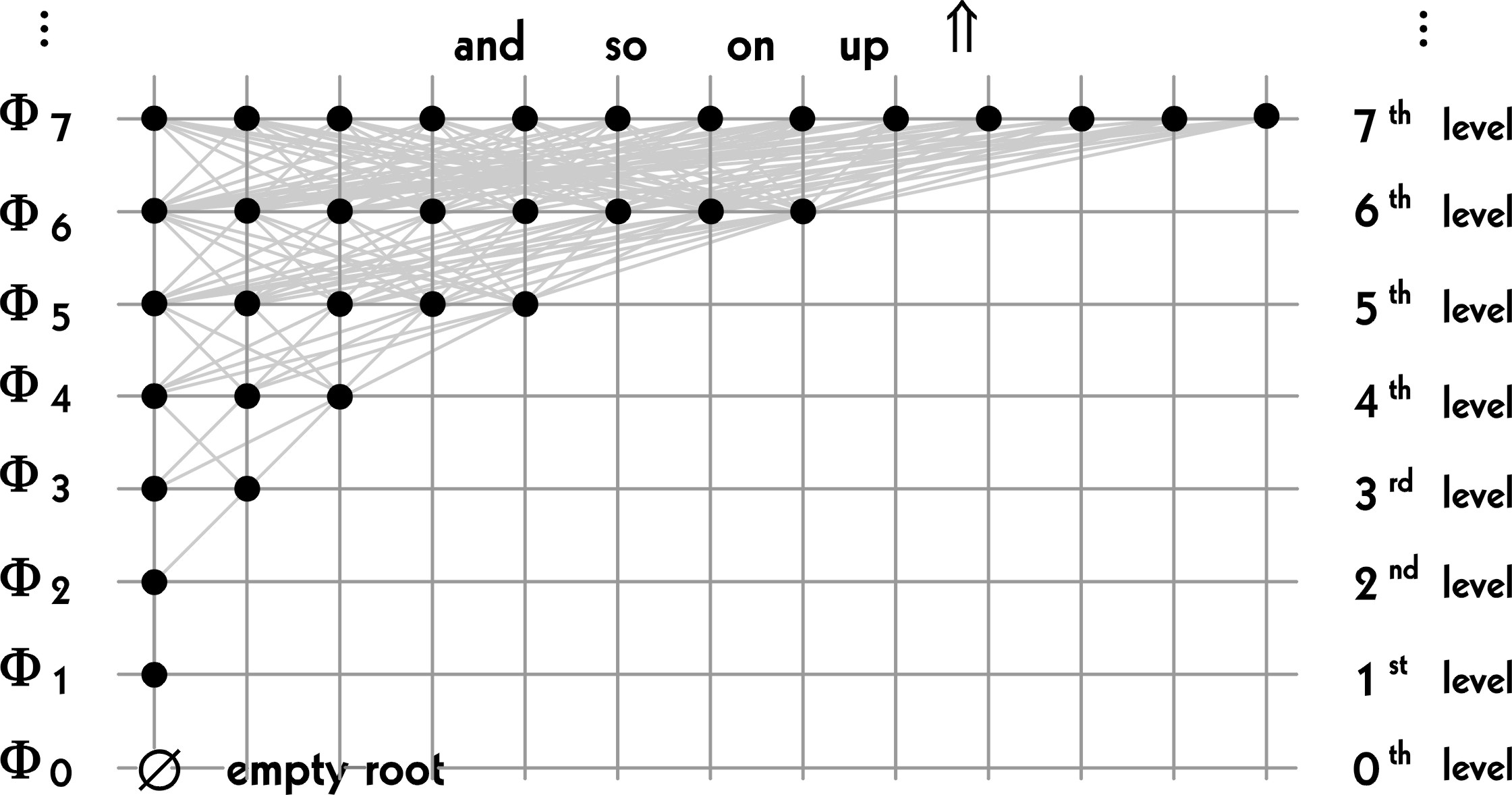
Figure 1: The $s$-th level in $\mathbb{N}\times\mathbb{N}\cup\{0\}$

In Kwaśniewski’s cobweb posets’ tiling problem one considers finite cobweb sub-posets for which we have finite number of levels in layer $\langle\Phi_{k}\rightarrow\Phi_{n}\rangle$, where $k\leq n$, $k,n\in\mathbb{N}\cup\{0\}$ with exactly $k_{j}$ vertices on $\Phi_{j}$ level $k\leq j\leq n$. For $k=0$ the sub-posets $\langle\Phi_{0}\rightarrow\Phi_{n}\rangle$ are named prime cobweb posets and these are those to be used - up to permutation of levels equivalence - as a block to partition finite cobweb sub-poset.

For the sake of combinatorial interpretation a natural numbers’ valued sequence $F$ which determines its’ cobweb poset has to be cobweb-admissible.

Figure 2: Display of four levels of Fibonacci numbers’ finite Cobweb sub-poset

Figure 3: Display of Natural numbers’ finite prime Cobweb poset

$F_{0}=0$ being acceptable as $0_{F}!\equiv F_{0}!=1$. We adopt then the convention to call the root $\{\emptyset\}$ the ”empty root”.

One of the problems posed in [6-8] is the one, which is the subject of [1].

The tiling problem

Suppose now that $F$ is a cobweb admissible sequence. Under which conditions any layer $\langle\Phi_{n}\!\rightarrow\!\Phi_{k}\rangle$ may be partitioned with help of max-disjoint blocks of established type $\sigma P_{m}$? Find effective characterizations and/or find an algorithm to produce these partitions.

The above Kwaśniewski [7,6] tiling problem is first of all the problem of existence of a partition of layer $\langle\Phi_{k}\rightarrow\Phi_{n}\rangle$ with max-disjoint blocks of the form $\sigma P_{m}$ defined as follows:

$$\sigma P_{m}=C_{m}[F,\sigma\langle F_{1},F_{2},\ldots,F_{m}\rangle]$$

It means that the partition may contain only primary cobweb sub-posets or these obtained from primary cobweb poset $P_{m}$ via permuting its levels as illustrated below (Fig. 4).

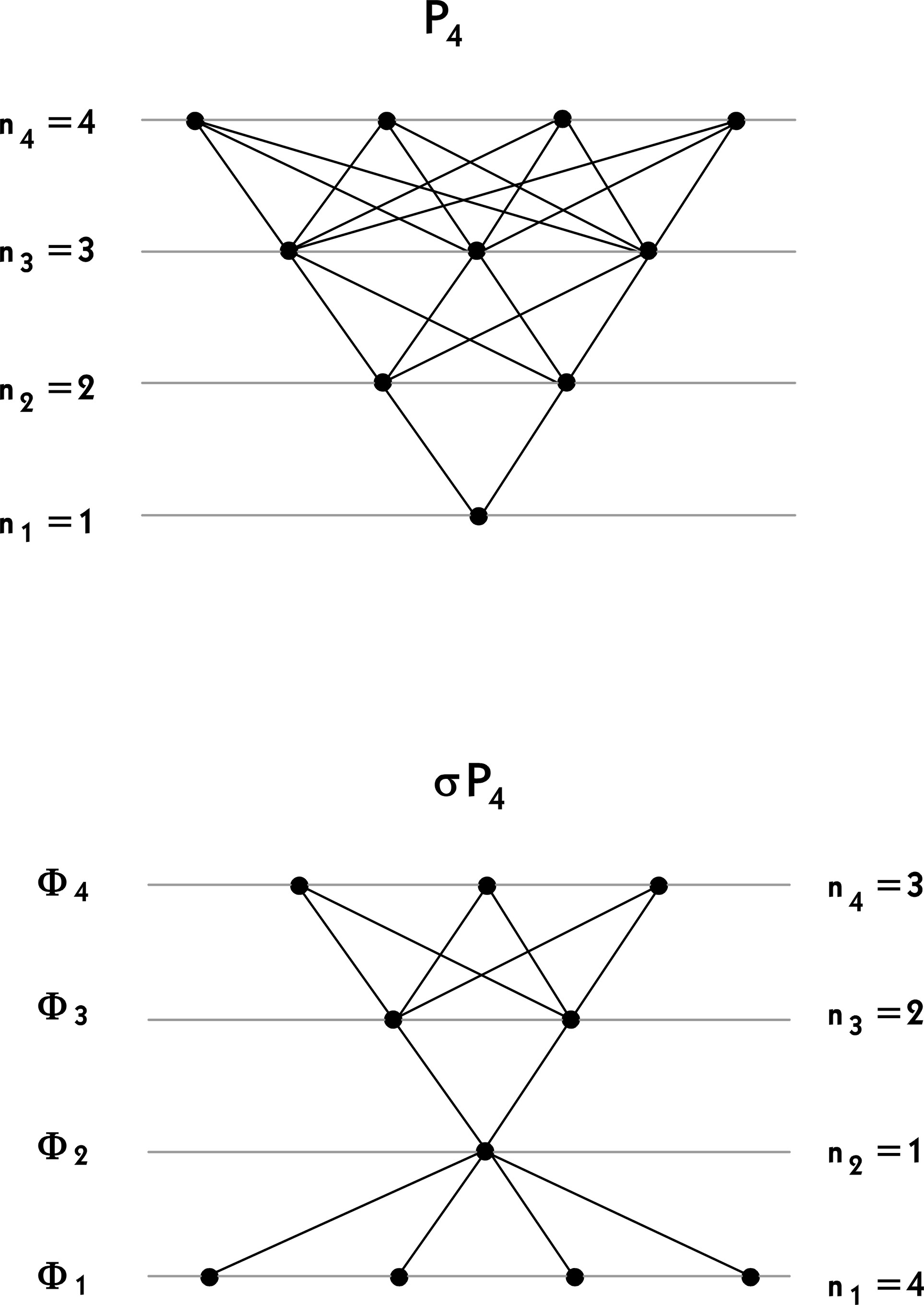
Figure 4: Display of block $\sigma P_{m}$ obtained from $P_{m}$ and permutation $\sigma$

The second author presents in [1] an algorithm to create a partition of any layer $\langle\Phi_{k}\rightarrow\Phi_{n}\rangle$, $k\leq\nolinebreak n$, $k,n\in\mathbb{N}\cup\{0\}$ of finite cobweb sub-poset specified by such $F$-sequences as Natural numbers and Fibonacci numbers. In [1] the following Theorem 1 and Theorem 2 are proved.

Theorem 2 (Natural numbers)

Consider any layer $\langle\Phi_{k+1}\rightarrow\Phi_{n}\rangle$ with $m$ levels where $m=n-k$, $k\leq{n}$ and $k,n\in\mathbb{N}\cup\{0\}$ in a finite cobweb sub-poset, defined by the sequence of natural numbers i.e. $F\equiv\{n_{F}\}_{n\geq 0},\ n_{F}=n,\ \linebreak n\in\mathbb{N}\cup\{0\}$. Then there exists at least one way to partition this layer with help of max-disjoint blocks of the form $\sigma P_{m}$.

Max-disjoint means that the two blocks have no maximal chain in common.

Before proving let us notice that for any $m,k\in\mathbb{N}$ such that $m+k=n$:

(2) $$n_{F}=m_{F}+k_{F}$$

where $1_{F}=1$.

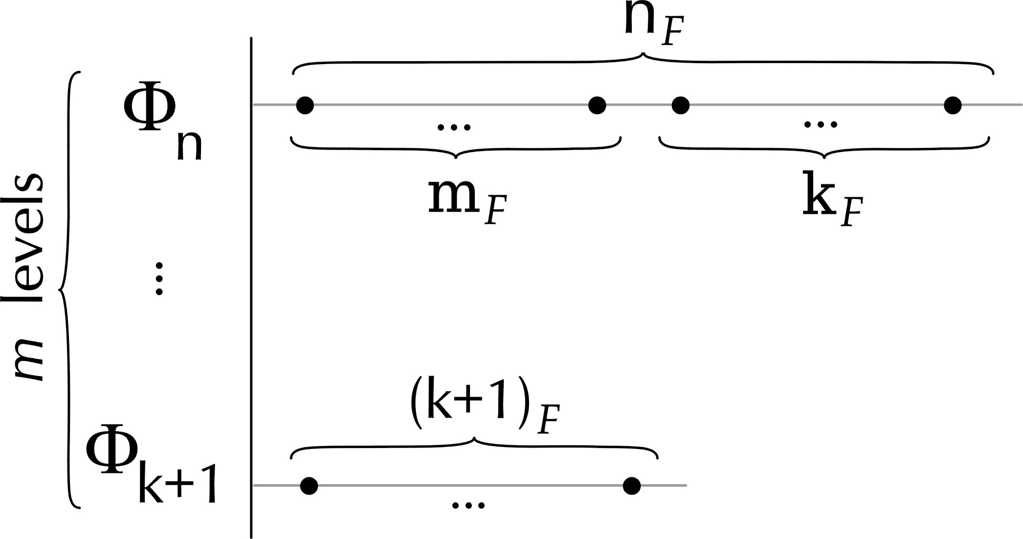
Figure 5: Picture of $m$ levels of Cobweb poset’ Hasse diagram

PROOF (cprta1) algorithm

Steep 1. There are $n_{F}=m_{F}+k_{F}$ vertices on the $\Phi_{n}$ level. Let us separate them by cutting into two disjoint subsets as illustrated by the Fig.5 and cope at first with $m_{F}$ vertices (Steep 2). Then we shall cope with those $k_{F}$ vertices left (Steep 3).

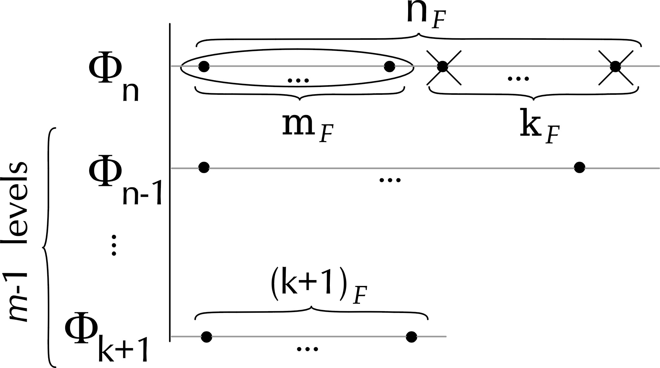
Figure 6: Picture of Steep 2

Steep 2. Temporarily we have $m_{F}$ fixed vertices on $\Phi_{n}$ level to consider. Let us cover them by $m$-th level of block $P_{m}$, which has exactly $m_{F}$ vertices-leafs. What was left is the layer $\langle\Phi_{k+1}\rightarrow\Phi_{n-1}\rangle$ and we might eventually partition it with smaller max-disjoint blocks $\sigma P_{m-1}$, but we need not to do that. See the next step.

Steep 3. Consider now the second complementary situation, where we have $k_{F}$ vertices on $\Phi_{n}$ level being fixed. Observe that if we move this level lower than $\Phi_{k+1}$ level, we obtain exactly $\langle\Phi_{k}\rightarrow\Phi_{n-1}\rangle$ layer to be partitioned with max-disjoint blocks of the form $\sigma P_{m}$. This ”move” operation is just permutation of levels’ order.

The layer $\langle\Phi_{k+1}\!\!\rightarrow\!\Phi_{n}\rangle$ may be partitioned with $\sigma P_{m}$ blocks if $\langle\Phi_{k+1}\!\rightarrow\nolinebreak\Phi_{n-1}\rangle$ may be partitioned with $\sigma P_{m-1}$ blocks and $\langle\Phi_{k}\!\!\rightarrow\Phi_{n-1}\rangle$ by $\sigma P_{m}$ again. Continuing these steeps by induction, we are left to prove that $\langle\!\Phi_{k}\!\rightarrow\Phi_{k}\rangle$ may be partitioned by $\sigma P_{1}$ blocks and $\langle\Phi_{1}\!\!\rightarrow\!\Phi_{m}\rangle$ by $\sigma P_{m}$ blocks which is obvious $\blacksquare$

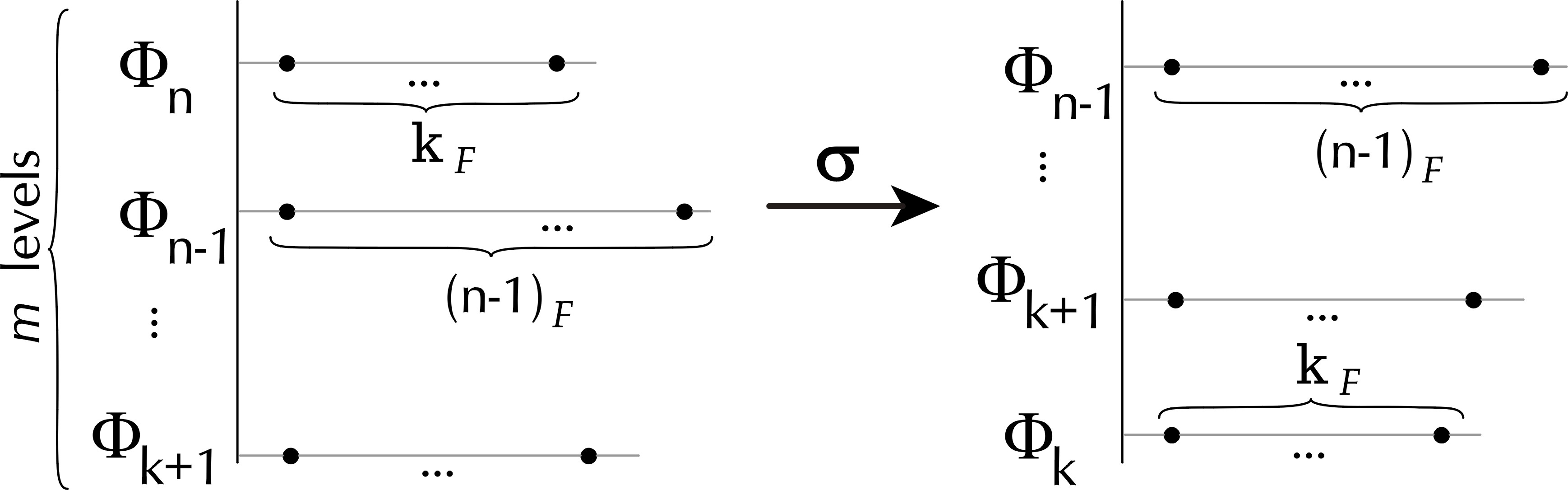
Figure 7: Picture of Steep 3

Observation 5

We already know from [7,6] that the number of max-disjoint equip-copies of $\sigma P_{m}$, rooted at the same fixed vertex of $k$-th level and ending at the $n$-th level is equal to

$${n\choose k}_{F}={n\choose m}_{F}$$

If we cut-separate family of leafs of the layer $\langle\Phi_{k+1}\!\!\rightarrow\Phi_{n}\rangle$, as in the proof of the Theorem 1 then the number of max-disjoint equip copies of $P_{m-1}$ from the Steep 2 is equal to

$${n-1\choose k}_{F}$$

However the number of max-disjoint equip copies of $P_{m}$ from the Steep 3 is equal to

$${n-1\choose k-1}_{F}$$

It results in formula of Newton’s symbol recurrence:

$${n\choose k}_{F}={n-1\choose k}_{F}+{n-1\choose k-1}_{F}$$

in accordance with what was expected for the case $F=\mathbb{N}$ thus illustrating the combinatorial interpretation from [7,6] in this particular case.

In the next we adapt Knuth notation for ”$F$-Stirling numbers” of the second kind $\Big{\{}{n\atop k}\Big{\}}_{F}$ as in [6] and also in conformity with Kwaśniewski notation for $F$-nomial coefficients [9-13,4]. The number of those partitions which are obtained via (cprta1) algorithm shall be denoted by the symbol $\Big{\{}{n\atop k}\Big{\}}_{F}^{1}$.

Observation 6

Let $F$ be a sequence matching (2). Then the number $\Big{\{}{n\atop k}\Big{\}}_{F}^{1}$ of different partitions of the layer $\langle\Phi_{k}\!\!\rightarrow\Phi_{n}\rangle$ where $n,k\in\mathbb{N},\ n,k\geq 1$ is equal to:

$$\bigg{\{}{n\atop k}\bigg{\}}_{F}^{1}={n_{F}\choose m_{F}}\cdot\bigg{\{}{n-1\atop k}\bigg{\}}_{F}^{1}\cdot\bigg{\{}{n-1\atop k-1}\bigg{\}}_{F}^{1}$$

$(S_{N})$

where $\Big{\{}{n\atop n}\Big{\}}_{F}^{1}=\Big{\{}{n\atop n}\Big{\}}_{F}=1$, $\Big{\{}{n\atop 1}\Big{\}}_{F}^{1}=\Big{\{}{n\atop 1}\Big{\}}_{F}=1$, $m=n-k+1$.

PROOF

According to the Steep 1 of the proof of Theorem 1 we may choose on $\Phi_{n}$ level $m_{F}$ vertices out of $n_{F}$ ones in ${n_{F}\choose m_{F}}$ ways. Next recurrent steps of the proof of Theorem 1 result in formula ($S_{N}$) via product rule of counting. $\blacksquare$

Note. $\Big{\{}{n\atop k}\Big{\}}_{F}^{1}$ is not the number of all different partitions of the layer $\nolinebreak{\langle\Phi_{k}\!\!\rightarrow\!\Phi_{n}\rangle}$ i.e. $\Big{\{}{n\atop k}\Big{\}}_{F}\geq\Big{\{}{n\atop k}\Big{\}}_{F}^{1}$ as computer experiments [6] show. There are much more other tilings with blocks $\sigma P_{m}$.

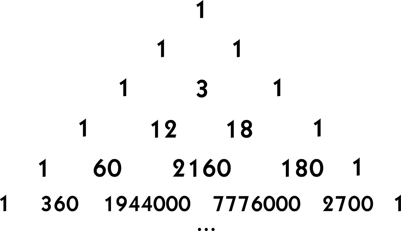
Figure 8: Natural numbers’ Cobweb poset tiling triangle of $\Big{\{}{n\atop k}\Big{\}}_{F}^{1}$

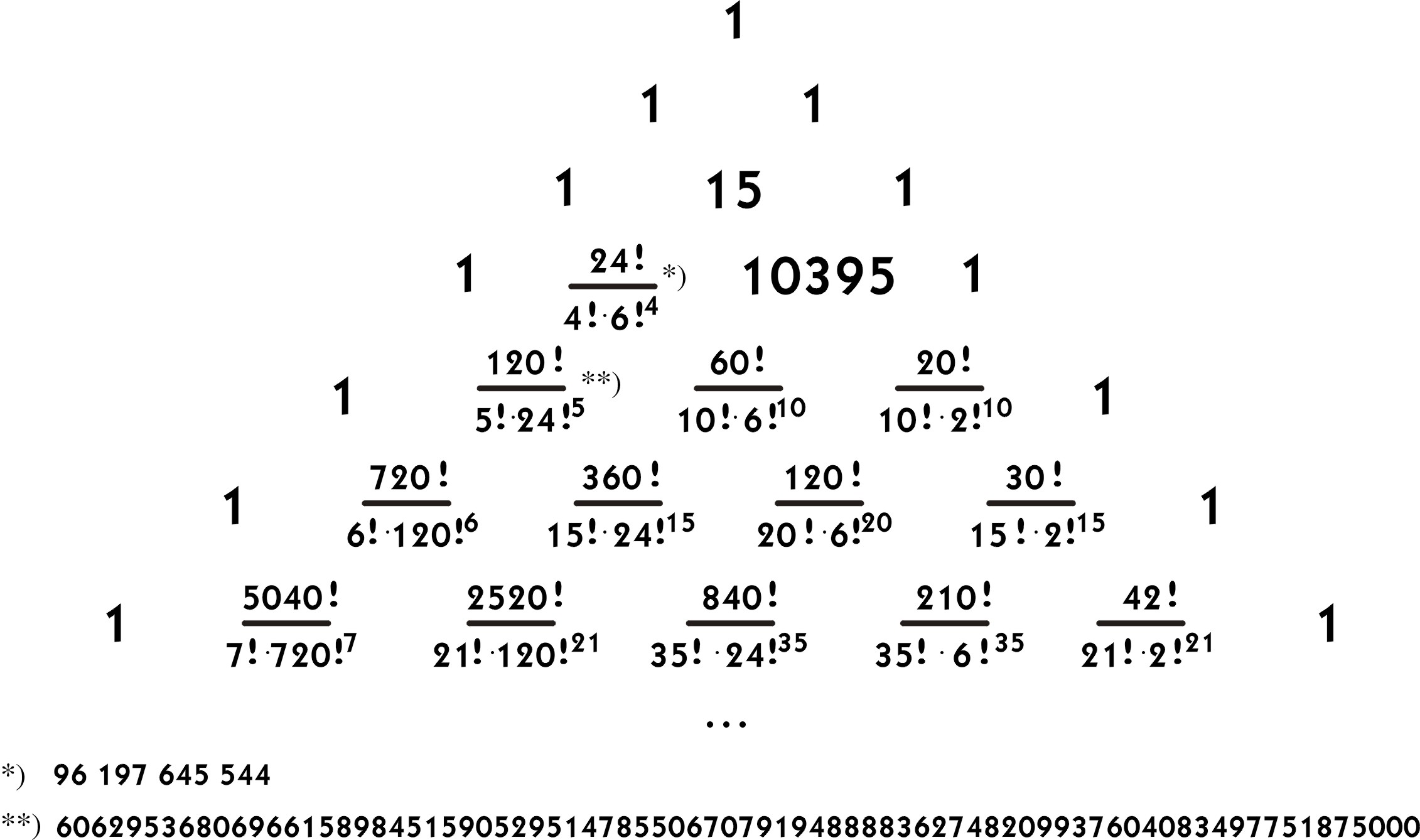
Figure 9: Kwaśniewski Natural numbers’ cobweb poset tiling triangle of $\Big{\{}{\eta\atop\kappa}\Big{\}}_{\lambda}$

This is to be compared with Kwaśniewski cobweb triangle [6] (Fig. 9) for the infinite triangle matrix elements

$$\Big{\{}{\eta\atop\kappa}\Big{\}}_{\lambda}=\delta_{\eta,\kappa\lambda}\frac{\eta!}{\kappa!\lambda!^{\kappa}}$$

counting the number of partitions with block sizes all equal to $\lambda$.

Here $const=\lambda=m_{F}!,m=n-k+1$ and

$$\eta=n_{F}^{\underline{m}},\ \ \kappa={n\choose k-1}_{F}$$

The numbers appearing above in $n$-th row, $n>3$ are GIANT numbers as seen from Fig.9.

The inequality $\Big{\{}{n\atop k}\Big{\}}_{F}^{1}\leq\Big{\{}{\eta\atop\kappa}\Big{\}}_{\lambda}$ gives us the rough upper bound for the number of tilings with blocks of established type $\sigma P_{m}$.

Theorem 3 (Fibonacci numbers)

Consider any layer $\langle\Phi_{k+1}\rightarrow\Phi_{n}\rangle$ with $m$ levels where $m=n-k$, $k\leq n$ and $k,n\in\mathbb{N}\cup\{0\}$ in a finite cobweb sub-poset, defined by the sequence of Fibonacci numbers i.e. $F\equiv\{n_{F}\}_{n\geq 0},n_{F}\in\mathbb{N}\cup\{0\}$. Then there exists at least one way to partition this layer with help of max-disjoint blocks of the form $\sigma P_{m}$.

The proof of the Theorem 2 for the Fibonacci sequence $F$ is similar to the proof of Theorem 1. We only need to notice that for any $m,k\in\mathbb{N}$, $m>1$, $m+k=n$ the following identity takes place:

(3) $$n_{F}=(m+k)_{F}=(k+1)_{F}\cdot m_{F}+(m-1)_{F}\cdot k_{F}$$

where $1_{F}=2_{F}=1$.

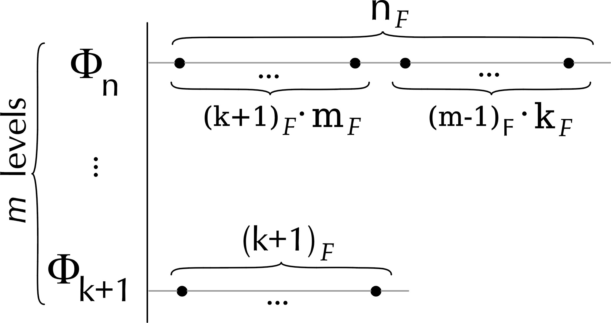
Figure 10: Picture of $m$ levels’ layer of Fibonacci Cobweb graph

PROOF

The number of leafs on the $\Phi_{n}$ layer is the sum of two summands $\kappa\cdot m_{F}$ and $\mu\cdot k_{F}$, where $\kappa=(k+1)_{F}$, $\mu=(m-1)_{F}$, (Fig. 10) therefore as in the proof of the Theorem 1 we consider two parts. At first we have to partition $\kappa$ layers $\langle\Phi_{k+1}\rightarrow\Phi_{n-1}\rangle$ with blocks $\sigma P_{m-1}$ and $\mu$ layers $\langle\Phi_{k}\rightarrow\Phi_{n-1}\rangle$ with $\sigma P_{m}$. The rest of the proof goes similar as in the case of the Theorem 1 $\blacksquare$

Theorem 2 is a generalization of Theorem 1 corresponding to $const=\kappa,\mu=1$ case.

Observation 7

The number of max-disjoint equip copies of $P_{m-1}$ which partition $\kappa$ layers $\langle\Phi_{k+1}\rightarrow\Phi_{n-1}\rangle$ is equal to

$$\kappa{n-1\choose k}_{F}=(k+1)_{F}{n-1\choose k}_{F}$$

However this number of max-disjoint equip copies of $P_{m}$ which partition $\mu$ layers $\langle\Phi_{k}\rightarrow\Phi_{n-1}\rangle$ is equal to

$$\mu{n-1\choose k-1}_{F}=(m-1)_{F}{n-1\choose k-1}_{F}$$

Therefore the sum corresponding to the Step 2 and to the Step 3 is the well known recurrence relation for Fibonomial coefficients [11,7,6,4]

$${n\choose k}_{F}=(k+1)_{F}{n-1\choose k}_{F}+(m-1)_{F}{n-1\choose k-1}_{F}$$

in accordance with what was expected for the case $F$ being now Fibonacci sequence thus illustrating the combinatorial interpretation from [6,7] in this particular case.

Observation 8

Let $F$ be a sequence matching (3). Then the number $\Big{\{}{n\atop k}\Big{\}}_{F}^{1}$ of different partitions of the layer $\langle\Phi_{k}\rightarrow\Phi_{n}\rangle$ where $n,k\in\mathbb{N},n,k\geq 1$ is equal to:

$$\bigg{\{}{n\atop{k}}\bigg{\}}_{F}^{1}=\frac{F_{n}!}{(F_{m}!)^{\kappa}\cdot(F_{k-1}!)^{\mu}}\cdot\bigg{\{}{n-1\atop k}\bigg{\}}_{F}^{1}\cdot\bigg{\{}{n-1\atop k-1}\bigg{\}}_{F}^{1}$$

$(S_{F})$

where $\Big{\{}{n\atop n}\Big{\}}_{F}^{1}=\Big{\{}{n\atop n}\Big{\}}_{F}=1$, $\Big{\{}{n\atop n-1}\Big{\}}_{F}^{1}=\Big{\{}{n\atop n-1}\Big{\}}_{F}=1$, $\Big{\{}{n\atop 1}\Big{\}}_{F}^{1}=\Big{\{}{n\atop 1}\Big{\}}_{F}=1$, $\kappa=k_{F},\mu=(m-1)_{F},m=n-k+1$, $F_{n}!=1\cdot 2\cdot\ldots\cdot(n_{F}-1)\cdot n_{F}$.

PROOF

According to the Steep 1 of the proof of Theorem 2 we may choose on $n$-th level $m_{F}$ vertices $\kappa$ times and next $(k-1)_{F}$ vertices $\mu$ times out of $n_{F}$ ones in $\frac{F_{n}!}{(F_{m}!)^{\kappa}\cdot(F_{k-1}!)^{\mu}}$ ways. Next recurrent steps of the proof of Theorem 2 result in formula ($S_{F}$) via product rule of counting $\blacksquare$

Observation 4 becomes Observation 2 once we put $const=\kappa,\mu=1$.

Easy example

For cobweb-admissible sequences $F$ such that $1_{F}=2_{F}=1$, $\Big{\{}\!{n\atop n-1}\!\Big{\}}_{F}^{1}\!\!\!=\!\!\Big{\{}\!{n\atop n-1}\!\Big{\}}_{F}\!\!\!=\!1$ as obviously we deal with the perfect matching of the bipartite graph which is very exceptional case (Fig. 11).

Note. As in the case of Natural numbers for $F$-Fibonacci numbers $\Big{\{}{n\atop 1}\Big{\}}_{F}^{1}$ is not the number of all different partitions of the layer $\langle\Phi_{k}\rightarrow\Phi_{n}\rangle$ i.e. $\Big{\{}{n\atop k}\Big{\}}_{F}\geq\Big{\{}{n\atop k}\Big{\}}_{F}^{1}$ as computer experiments [6] show. There are much more other tilings with blocks $\sigma P_{m}$.

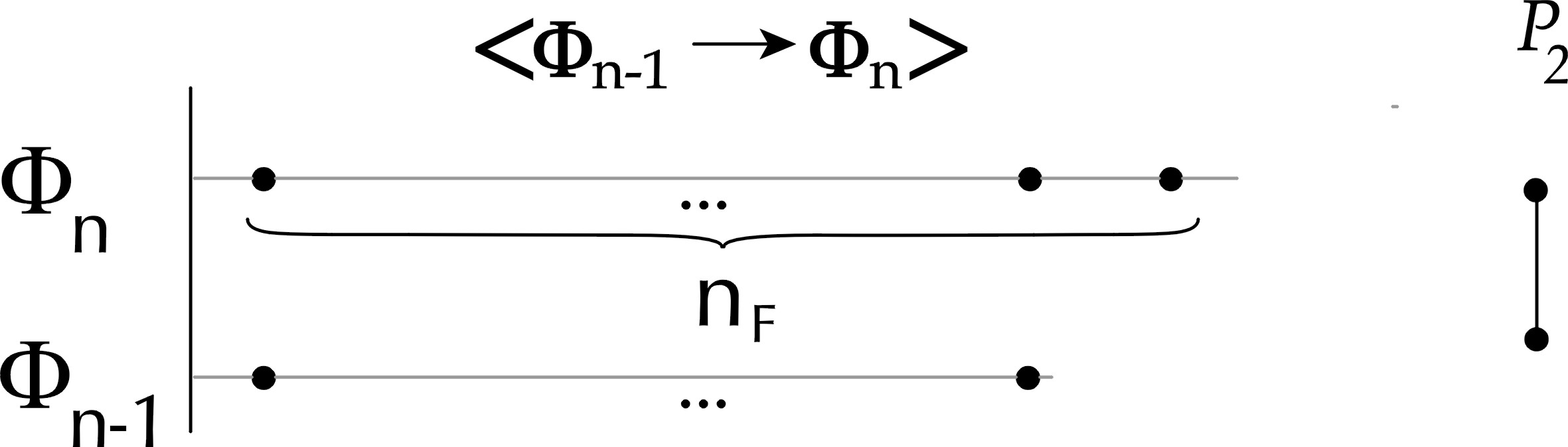
Figure 11: Easy example picture

This is to be compared with Kwaśniewski [6] cobweb triangle for the infinite triangle matrix elements (Fig. 13)

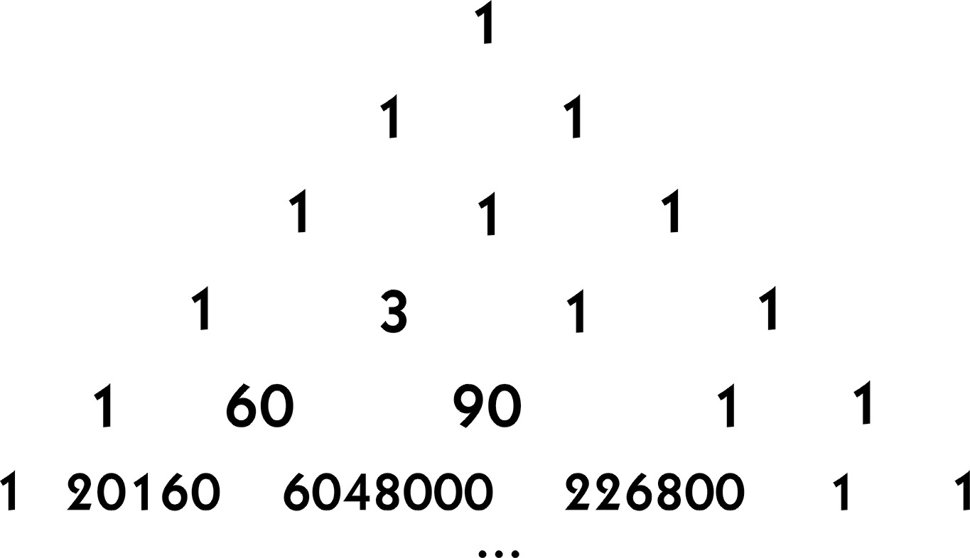
Figure 12: Fibonacci numbers’ cobweb poset tiling triangle of $\Big{\{}{n\atop k}\Big{\}}_{F}^{1}$

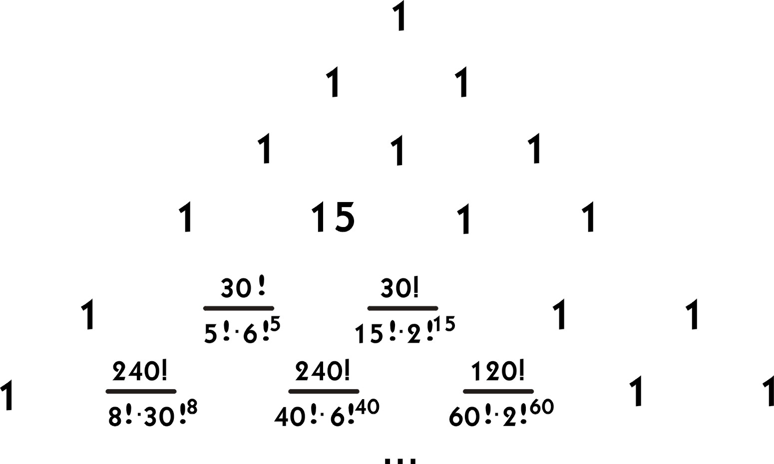
Figure 13: Kwaśniewski Fibonacci numbers’ cobweb tiling triangle of $\Big{\{}{\eta\atop\kappa}\Big{\}}_{\lambda}$

4 Other tiling sequences

Definition 8

The cobweb admissible sequences that designate cobweb posets with tiling are called cobweb tiling sequences.

4.1 Easy examples

The above method applied to prove tiling existence for Natural and Fibonacci numbers relies on the assumptions (2) or (3). Obviously these are not the only sequences that do satisfy recurrences (2) or (3). There exist also other cobweb tiling sequences beyond the above ones with different initial values.

There exist also cobweb admissible sequences determining cobweb poset with no tiling of the type considered in this paper.

Example 1

$n_{F}=(m+k)_{F}=m_{F}+k_{F}$, $n\geq 1$ ( $0_{F}$ = corresponds to one ”empty root” $\{\emptyset\}$)

This might be considered a sample example illustrating the method. For example if we choose $1_{F}=c\in\mathbb{N}$, we obtain the class of sequences $n_{F}=c\cdot n$ for $n\geq 1$. Naturally layers of such cobweb posets designated by the sequence satisfying (2) for $n\geq 1$ may also be partitioned according to (cprta1).

Example 1.5 $1_{F}=1,n_{F}=c\cdot n,n>1$ ($0_{F}$ = corresponds to one ”empty root” $\{\emptyset\}$ ) This might be considered another sample example now illustrating the ”shifted” method named (cpta2). For example if we choose $2_{F}=c\in\mathbb{N}$, while $1_{F}=1$, we obtain the class of sequences $1_{F}=1$ and $n_{F}=c\cdot n$ for $n>1$. Layers of such cobweb posets designated by these sequences may also be partitioned.

Observation 9

Algorithm (cpta2) Given any (including cobweb-admissible) sequence $A\equiv\{n_{A}\}_{n\geq 0}$, $s\in\mathbb{N}\cup\{0\}$ let us define shift unary operation $\oplus_{s}$ as follows:

$$\oplus_{s}A=B,\qquad n_{B}=\left\{\begin{array}[]{ll}1&n<s\\ (n-s)_{A}&n\geq s\end{array}\right.$$

where $B\equiv\{n_{B}\}_{n\geq 0}$. Naturally $\oplus_{0}$ = identity. Then the following is true. If a sequence $A$ is cobweb-tiling sequence then $B$ is also cobweb-tiling sequence.

For example this is the case for $A=1,2,3,4,\ldots$, $\oplus_{3}A=1,1,1,1,2,3,4,\ldots$.

Example 2

$n_{F}=m_{F}\cdot k_{F}$

If we choose $1_{F}=c\in\mathbb{N}$, we obtain the class of sequences $n_{F}=c^{n},n\geq 0$. We can also consider more general case $n_{F}=\alpha\cdot m_{F}\cdot k_{F}$, where $\alpha\in\mathbb{N}$ which gives us the next class of tiling sequences $n_{F}=\alpha^{n-1}\cdot c^{n},n\geq 1,0_{F}=1$ and layers of such cobweb posets can be partitioned by (cprta1) algorithm. For example: $1_{F}=1,\alpha=2\rightarrow F=1,1,2,4,8,16,32,\ldots$ or $1_{F}=2\rightarrow F=1,2,4\alpha,8\alpha^{2},16\alpha^{3},\ldots$

Example 3

$n_{F}=(m+k)_{F}=(k+1)_{F}\cdot m_{F}+(m-1)_{F}\cdot k_{F}$

Here also we have infinite number of cobweb tiling sequences depending on the initial values chosen for the recurrence $(k\!+\!2)_{F}\!=\!2_{F}(k\!+\!1)_{F}\!+\!k_{F},k\!\!\geq\!\!0$. For example: $1_{F}=1$ and $2_{F}=2\rightarrow$ $F=1,2,5,12,29,70,169,408,985,\ldots$ Note that this is not shifted Fibonacci sequence as we use recurrence (2) which depends on initial conditions adopted. Next $1_{F}=1$ and $2_{F}=3\rightarrow F=1,3,10,33,109,360,1189,\ldots$ Note that this is not remarcable Lucas sequence [7].

Neither of sequences: shifted Fibonacci nor Lucas sequence satisfy (2) neither these (as well as the Catalan, Motzkin, Bell or Euler numbers sequences) are cobweb admissible sequences. This indicates the further exceptionality of Fibonacci sequence along with natural numbers.

The proof of tiling existence leads to many easy known formulas for sequences, where we use multiplications of terms $m_{F}$ and/or $k_{F}$, like $n_{F}=\alpha\cdot k_{F}$, $n_{F}=\alpha\cdot m_{F}k_{F}$, $n_{F}=\alpha\cdot(m\pm\beta)_{F}k_{F}$, where $\alpha,\beta\in\mathbb{N}$, $n=m+k$ and so on.

This are due to the fact that in the course of partition’s existence proving with (cprta1) partition of layer $\langle\Phi_{k+1}\!\rightarrow\!\Phi_{n}\rangle$ existence relies on partition’s existence of smaller layers $\langle\Phi_{k+1}\!\rightarrow\!\Phi_{n-1}\rangle$ and/or $\langle\Phi_{k}\!\rightarrow\!\Phi_{n-1}\rangle$.

In what follows we shall use an at the point product of two cobweb-admissible sequences giving as a result a new cobweb admissible sequence - cobweb tiling sequences included to which the above described treatment (cprta1) applies.

4.2 Beginnings of the cobweb-admissible sequences production

Definition 9

Given any two cobweb-admissible sequences $A\equiv\{n_{A}\}_{n\geq 0}$ and $B\equiv\{n_{B}\}_{n\geq 0}$, their at the point product $C$ is given by

$$A\cdot B=C\qquad C\equiv\{n_{C}\}_{n\geq 0},\ n_{C}=n_{A}\cdot n_{B}$$

It is obvious that $A\cdot B=C$ is also cobweb admissible and

$${n\choose k}_{A\cdot B}=\frac{n_{A}^{\underline{k}}}{k_{A}!}\cdot\frac{n_{B}^{\underline{k}}}{k_{B}!}={n\choose k}_{A}\cdot{n\choose k}_{B}\in\mathbb{N}\cup\{0\}$$

Example 4

Almost constant sequences $C_{t}$

$$C_{t}=\{n_{C}\}_{n\geq 0}\qquad\mathrm{where}\ const=n_{C}=t\in\mathbb{N}\ \mathrm{for}\ n>0,0_{F}=1.$$

as for example $C_{5}=1,5,5,5,5,\ldots$ are trivially cobweb-admissible and cobweb tiling sequences - see next example.

In the following $I$ denotes unit sequence $I\equiv\{1\}_{n\geq 0}$; $I\cdot{A}=A$.

Example 5

Not diminishing sequence $A_{c,M}$

If we multiply $i$-th term (where $i\geq M\geq 1,M\in\mathbb{N}$) of sequence $I$ by any constant $c\in\mathbb{N}$, then the product cobweb admissible sequence is $A_{c,M}$.

$$A_{c,M}\equiv\{n_{A}\}_{n\geq 0}\qquad\mathrm{where}\ n_{A}=\left\{\begin{array}[]{lr}1&1\leq n<M\\ c&n\geq M\end{array}\right.$$

as for example $\nolinebreak{A_{5,10}=1,\underbrace{1,\ldots,1}_{10},5,5,5,\ldots}$ or more general example

$\nolinebreak{A_{3,2,10}=1,\underbrace{3,\ldots,3}_{10},6,6,6,\ldots}$ Clearly sequences of this type are cobweb admissible and cobweb tiling sequences.

Indeed. Each of level of layer $\langle\Phi_{k}\!\rightarrow\!\Phi_{n}\rangle$ has the same or more vertices than each of levels of the block $\sigma P_{m}$. If not the same then the number of vertices from the block $\sigma P_{m}$ divides the number of vertices at corresponding layer’s level. This is how (cprta2) applies.

Note. The sequence $A_{3,2,10}$ is a product of two sequences from Example 4, $A=1,3,3,3,3,3,3,\ldots$ and $B^{\prime}=\oplus_{10}B=1,\ldots,1,2,2,2,\ldots$ where $\\ B=1,2,2,2,2,2,2,\ldots$, then $A\cdot B^{\prime}=A_{3,2,10}=1,\underbrace{3,\ldots,3}_{10},6,6,6,\ldots$

Example 6

Periodic sequence $B_{c,M}$

A more general example is supplied by

$$B_{c,M}\equiv\{n_{B}\}_{n\geq 0}\qquad\mathrm{where}\ n_{B}=\left\{\begin{array}[]{ll}1&M\nmid{n}\vee n=0\\ c&M|n\end{array}\right.$$

where $c,M\in\mathbb{N}$. Sequences of above form are cobweb tiling, as for example $B_{2,3}=\underbrace{1,1,2}_{3},1,1,2,\ldots$, $B_{7,4}=\underbrace{1,1,1,7}_{4},1,1,1,7,\ldots$ Indeed.

PROOF Consider any layer $\langle\Phi_{k}\!\rightarrow\!\Phi_{n}\rangle$, $k\leq n$, $k,n\in\mathbb{N}\cup\{0\}$, with $m$ levels:

For $m<M$, the block $P_{m}$ has one vertex on each of levels. The tiling is trivial.

For $m\geq K$, the sequence $B_{c,M}$ has a period equal to $M$, therefore any layer of $m$ levels has the same or larger number of levels with $c$ vertices than the block $\sigma P_{m}$, if layer’s level has more vertices than corresponding level of block $\sigma P_{m}$ then the quotient of this numbers is a natural number i.e. $1|c$, thus the layer can be partitioned by one block $P_{m}$ or by $c$ blocks $\sigma P_{m}$ $\blacksquare$

Observation 10

The at the point product of the above sequences gives us occasionally a method to produce Natural numbers as well as expectedly other cobweb-admissible sequences with help of the following algorithm.

Algorithm for natural numbers’ generation (cta3)

$N(s)$ denotes a sequence which first $s$ members is next Natural numbers i.e. $N(s)\equiv\{n_{N}\}_{n\geq 0}$, where $n_{N}=n$, for $n=1,2,\ldots,s$, $\ p,p_{n}$ - prime numbers.

1. $N(1)=\mathbf{I}=1,1,1,\ldots$

2. $N(2)=N(1)\cdot B_{2,2}=1,2,1,2,1,2,\ldots$

3. $N(3)=N(2)\cdot B_{3,3}=1,2,3,2,1,6,\ldots$

4. $N(n)=N(n-1)\cdot\mathbf{X}$

Consider $n$:

1. let $n$ be prime, then $\neg\exists_{1\neq i\in[n-1]}i|n\Rightarrow n_{N}=1\Rightarrow\mathbf{X}=B_{n,n}$

2. let $n=p^{m}$, $1<m\in\mathbb{N}$, then $n_{N}=p^{m-1}\Rightarrow\mathbf{X}=B_{p,n}$

3. let $n=\prod_{s=1}^{u}p_{s}^{m_{s}}$, where $p_{i}\neq p_{j}$ for $i\neq j$, $m_{i}\geq 1$, $\\ i=1,2,\ldots,u$, $u>1$

   $\forall_{i\in[u]}p_{i}^{m_{i}}<n\Rightarrow n_{N}=\mathrm{LCD}\left(\{p_{i}^{m_{i}}:i=1,2,\ldots,u\}\right)$ $\\ \wedge\forall_{i\neq j}\mathrm{GCD}(p_{i}^{m_{i}},p_{j}^{m_{j}})=1$ $\Rightarrow$ $n_{N}=\prod_{s=1}^{u}p_{s}^{m_{s}}$ $\Rightarrow\mathbf{X}=\mathbf{I}$

where lowest common denominator or least common denominator (LCD) and greatest common divisor (GCD) abbreviations were used.

Concluding

$$N(n)=N(n-1)\cdot B_{h_{n},n}\begin{array}[]{c}\scriptstyle{n\rightarrow\infty}\\ \longrightarrow\\ \end{array}\mathbb{N}$$

$$h_{n}=\left\{\begin{array}[]{ll}p&\quad n=p^{m},\quad\mathbb{N}\ni m\geq 1\\ 1&\quad n=\prod_{s=1}^{u>1}p_{s}^{m_{s}},\quad\mathbb{N}\ni m_{s}\geq 1\end{array}\right.$$

while $\{h_{n}\}_{n\geq 1}=1,2,3,2,5,1,7,2,3,1,11,1,13,1,1,2,17,\ldots$

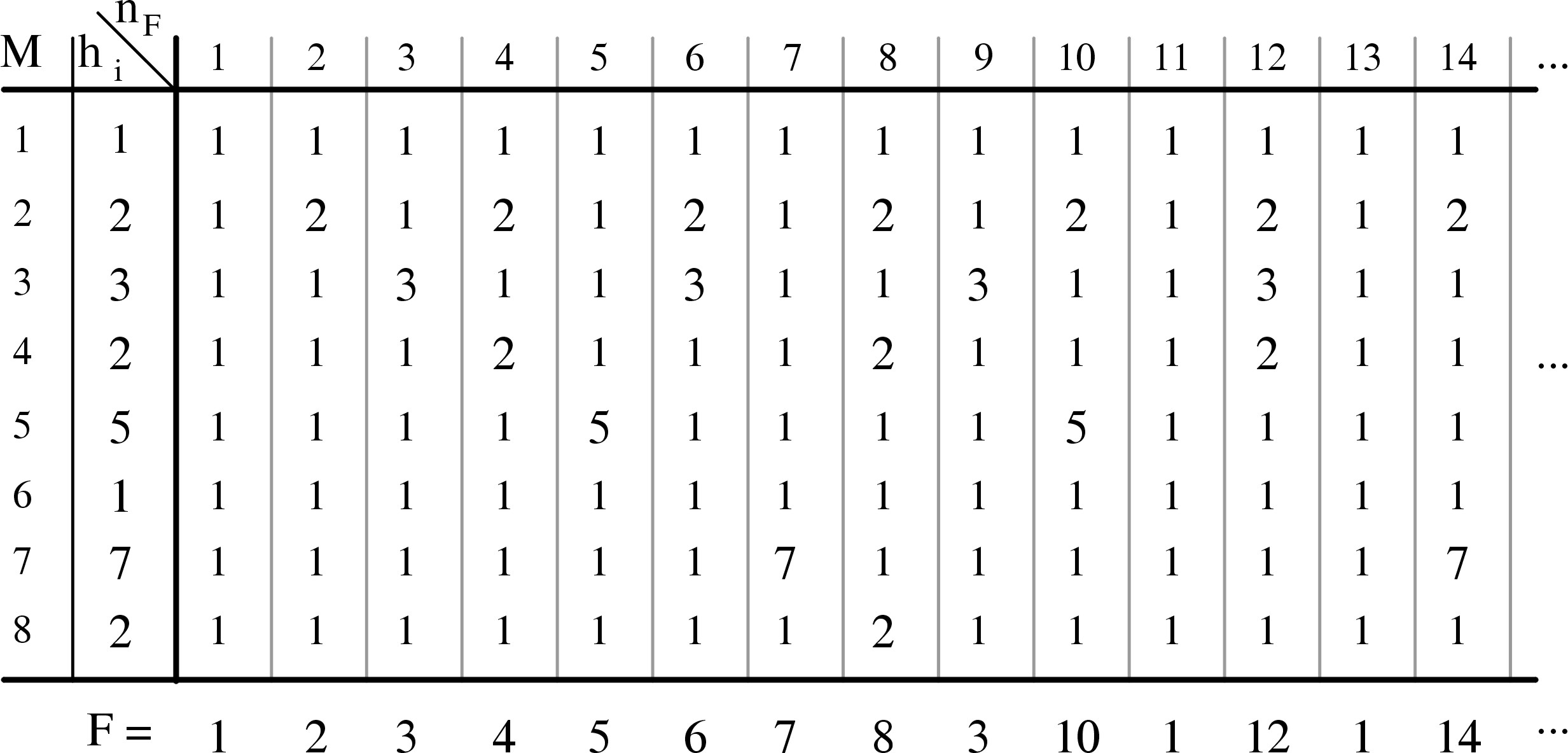
Figure 14: Display of eight steeps of algorithm (cta3)

As for the Fibonacci sequence we expect the same statement to be true for $n\rightarrow\infty$ bearing in mind those properties of Fibonacci numbers which make them an effective tool in Zeckendorf representation of natural numbers. For the Fibonacci numbers the would be sequence $\{h_{n}\}_{n\geq 1}$ is given by $\{h_{n}\}_{n\geq 1}=1,1,2,3,5,4,13,7,17,11,89,6,\ldots$

We end up with general observation - rather obvious but important to be noted.

Theorem 4

Not all cobweb-admissible sequences are cobweb tiling sequences.

PROOF

It is enough to give an appropriate example. Consider then a cobweb-admissible sequence $F=A\cdot B=1,2,3,2,1,6,1,2,3,\ldots$, where $A=1,2,1,2,1,2\ldots$ and $B=1,1,3,1,1,3,\ldots$ are both cobweb admissible and cobweb tiling. Then the layer $\langle\Phi_{5}\!\rightarrow\!\Phi_{7}\rangle$ can not be partitioned with blocks $\sigma P_{3}$ as the level $\Phi_{5}$ has one vertex, level $\Phi_{5}$ has six while $\Phi_{5}$ has one vertex again (Fig 15).

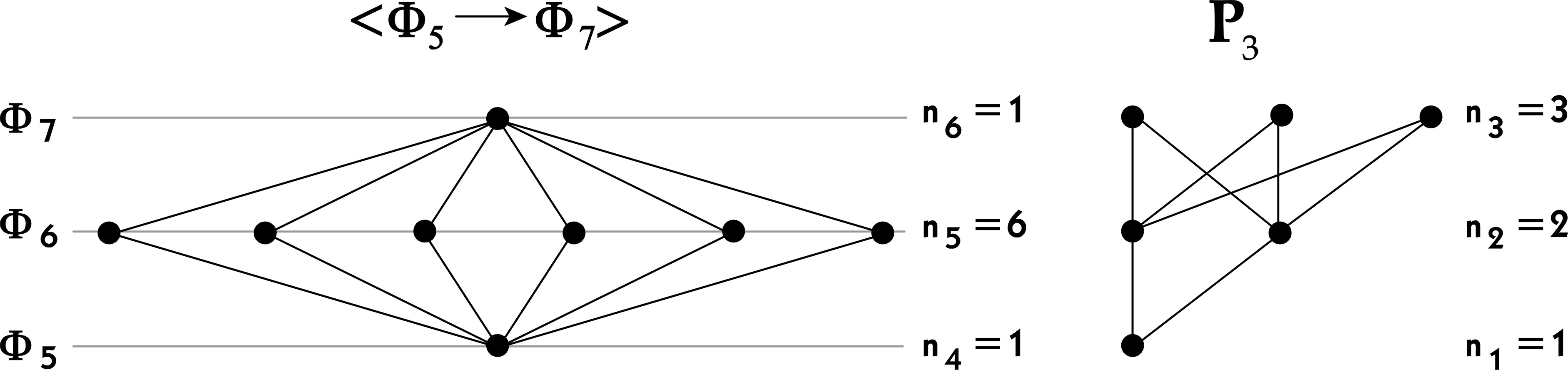
Figure 15: Picture proof of Theorem 3

Corollary The at the point product of two tiling sequences does not need to be a tiling sequence.

However for $A=1,2,1,2,\ldots$ and $B=1,1,3,1,1,3,\ldots$ cobweb tiling sequences their product $F=A\cdot B=1,2,3,2,1,6,1,\ldots$ is not a cobweb tiling sequence. A natural question - is it still ahead [6,7]? . Find the effective characterizations and or algorithms for a cobweb admissible sequence to be a cobweb tiling sequence. The second author has encoded the problem of an algorithm being looked for with help of his invention called by him ”‘Primary cobweb admissible binary tree”’ and this is a subject of a separate note to be presented soon.

5 GCD-morphism Problem. Problem III.

Coming over to the last problem announced above following [6-8] let us note that the Observation 4. provides us with the new combinatorial interpretation of the immense class of all classical $F-nomial$ coefficients including binomial or Gauss $q$- binomial ones or Konvalina generalized binomial coefficients of the first and of the second kind [3] - which include Stirling numbers of both kinds too. All these $F$-nomial coefficients naturally are computed with their correspondent cobweb-admissible sequences. More than that - the vast ‘umbral’ family of $F$-sequences [9-13,4] includes also those which are called ”GCD-morphic” sequences. This means that $GCD[F_{n},F_{m}]=F_{GCD[n,m]}$ where $GCD$ stays for Greatest Common Divisor.

Definition 10

. The sequence of integers $F=\{n_{F}\}_{n\geq 0}$ is called the GCD-morphic sequence if $GCD[F_{n},F_{m}]=F_{GCD[n,m]}$ where $GCD$ stays for Greatest Common Divisor operator.

The Fibonacci sequence is a much nontrivial [11,12,6] guiding example of GCD-morphic sequence. Of course not all incidence coefficients of reduced incidence algebra of full binomial type are computed with GCD-morphic sequences however these or that - if computed with the cobweb correspondent admissible sequences all are given the new, joint cobweb poset combinatorial interpretation via Observation 3. More than that - in [8] a prefab-like combinatorial description of cobweb posets is being served with corresponding generalization of the fundamental exponential formula.

Question: which of these above mentioned sequences are GCD-morphic sequences?

GCD-morphism Problem. Problem III. Find effective characterizations and/or an algorithm to produce the GCD-morphic sequences i.e. find all examples.

The second author has ”‘almost solved”’ the GCD-morphism Problem - again with help of his invention called by him ”‘Primary cobweb admissible binary tree”’ and this is a subject of a separate note to be presented soon.(See [27]).

6 Apendix

A.1. Cobweb posets and KoDAGs’ ponderables of Kwaśniewski relevant recent productions. [19-25,7,6]

Definition 11

Let $n\in N\cup\left\{0\right\}\cup\left\{\infty\right\}$. Let $r,s\in N\cup\left\{0\right\}$. Let $\Pi_{n}$ be the graded partial ordered set (poset) i.e. $\Pi_{n}=(\Phi_{n},\leq)=(\bigcup_{k=0}^{n}\Phi_{k},\leq)$ and $\left\langle\Phi_{k}\right\rangle_{k=0}^{n}$ constitutes ordered partition of $\Pi_{n}$. A graded poset $\Pi_{n}$ with finite set of minimal elements is called cobweb poset iff

$$\forall x,y\in\Phi\ i.e.\ x\in\Phi_{r}\ and\ y\in\Phi_{s}\ r\neq s\ \Rightarrow\ x\leq y\ or\ y\leq x,$$

$\Pi_{\infty}\equiv\Pi.$

Note. By definition of $\Pi$ being graded its levels $\Phi_{r}\in\left\{\Phi_{k}\right\}_{k}^{\infty}$ are independence sets and of course partial order $\leq$ up there in Definition 6.1. might be replaced by $<$.

The Definition 11 is the reason for calling Hasse digraph $D=\left\langle\Phi,\leq\cdot\right\rangle$ of the poset $(\Phi,\leq))$ a KoDAG as in Professor Kazimierz Kuratowski native language one word Komplet means complete ensemble - see more in [19-25].

Definition 12

Let $F=\left\langle k_{F}\right\rangle_{k=0}^{n}$ be an arbitrary natural numbers valued sequence, where $n\in N\cup\left\{0\right\}\cup\left\{\infty\right\}$. We say that the cobweb poset $\Pi=(\Phi,\leq)$ is denominated (encoded=labelled) by $F$ iff $\left|\Phi_{k}\right|=k_{F}$ for $k=0,1,...,n.$

A.2. See also much relevant [26,2011]

A.3. Cobweb posets and combinatorial interpretation in discrete hyper-boxes language.[19],[29]

Theorem. [19]
For $F$-cobweb admissible sequences $F$-binomial coefficient ${{n}\choose{k}}_{\!\!F}$ is the cardinality of the family of equipotent to $V_{0,m}$ mutually disjoint discrete hyper-boxes, all together partitioning the discrete hyper-box $V_{k+1,n}$ $\equiv$ the layer $\langle\Phi_{k+1}\to\Phi_{n}\rangle$, where $m=n-k$.

The cobweb tiling problem in the language of discrete hyper-boxes.

Comment General ”fractal-reminiscent” comment. The discrete $m$-dimensional $F$-box ($m=n-k$) with edges’ sizes designated by natural numbers’ valued sequence $F$ where invented in [26] as a response to the so called cobweb tiling problem posed in [6,2007] and then repeated in [7,2009]. This tiling problem was considered by Maciej Dziemiańczuk in [1,2008] where it was shown that not all admissible $F$-sequences permit tiling as defined in [6,2007]. Then - after [26,2009 ArXiv] this tiling problem was considered by Maciej Dziemiańczuk in discrete hyper-boxes language [28, 2009].

Recall the fact ([6,2007], [7,2009]): Let $F$ be an admissible sequence. Take any natural numbers $n,m$ such that $n\geq m$, then the value of $F$-binomial coefficient ${{n}\choose{k}}_{\!\!F}$ s equal to the number of sub-boxes that constitute a $\kappa$-partition of $m$-dimensional $F$-box $V_{m,n}$ where $\kappa=|V_{m}|$.

Definition 13

Let $V_{m,n}$ be a $m$-dimensional $F$-box. Then any $\kappa$-partition into sub-boxes of the form $V_{m}$ is called tiling of $V_{m,n}$.

Hence only these partitions of $m$-dimensional box $V_{m,n}$ are admitted for which all sub-boxes are of the form $V_{m}$ i.e. we have a kind of (self-similarity).

It was shown in [13, 2008] by Maciej Dziemiańczuk that the only admissibility condition is not sufficient for the existence a tiling for any given $m$-dimensional box $V_{k,n}$. Kwaśniewski in [6,2007] and [7,2009] posed the question called Cobweb Tiling Problem which we repeat here.

Tiling problem
Suppose that $F$ is an admissible sequence. Under which conditions any $F$-box $V_{m,n}$ designated by sequence $F$ has a tiling? Find effective characterizations and/or find an algorithm to produce these tilings.

In [28, 2009] by Maciej Dziemiańczuk one proves the existence of such tiling for certain sub-family of admissible sequences $F$. These include among others $F=$ Natural numbers, Fibonacci numbers, or $F=\left\langle n_{q}\right\rangle_{n\geq 0}$ Gaussian sequence. Original extension of the above tiling problem onto the general case multi $F$-multinomial coefficients is proposed in [28, 2009] , too. Moreover - a reformulation of the present cobweb tiling problem into a clique problem of a graph specially invented for that purpose - is invented.

References

- [1] Maciej Dziemiańczuk, On Cobweb posets tiling problem, Adv. Stud. Contemp. Math. volume 16 (2), (2008): 219-233. arXiv:0709.4263v2, Thu, 4 Oct 2007 14:13:44 GMT
- [2] Charles Jordan On Stirling Numbers T hoku Math. J. 37 (1933),254-278.
- [3] John Konvalina , A Unified Interpretation of the Binomial Coefficients, the Stirling Numbers and the Gaussian Coefficients The American Mathematical Monthly 107 (2000), 901-910.
- [4] Ewa Krot, An Introduction to Finite Fibonomial Calculus, CEJM 2(5) (2005) 754-766.
- [5] Ewa Krot, The first ascent into the Fibonacci Cob-web Poset, Adv. Stud. Contemp. Math. 11 (2) (2007) 179-184.
- [6] A. Krzysztof Kwaśniewski, Cobweb posets as noncommutative prefabs, Adv. Stud. Contemp. Math. vol.14 (1) (2007): 37 - 47. arXiv:math/0503286v4 [v4] Sun, 25 Sep 2005 23:40:37 GMT
- [7] A. Krzysztof Kwaśniewski, On cobweb posets and their combinatorially admissible sequences, Advanced Studies in Contemporary Mathematics, 18 no. 1, (2009): 17-32. arXiv:math/0512578v5, [v5] Mon, 19 Jan 2009 21:47:32 GMT
- [8] A. Krzysztof Kwaśniewski, First observations on Prefab posets’ Whitney numbers, Advances in Applied Clifford Algebras Volume 18, Number 1 / February, 2008, 57-73, Xiv:0802.1696v1, [v1] Tue, 12 Feb 2008 19:47:18 GMT
- [9] A. Krzysztof Kwaśniewski,On extended finite operator calculus of Rota and quantum groups Integral Transforms and Special Functions, 2 (4) (2001) 333-340.
- [10] A. Krzysztof Kwaśniewski, Main theorems of extended finite operator calculus Integral Transforms and Special Functions, 14 (6) (2003) 499-516.
- [11] A. Krzysztof Kwaśniewski, The Logarithmic Fib-Binomial Formula, Adv. Stud. Contemp. Math. v.9 No.1 (2004): 19 -26. arXiv:math/0406258v1 [v1] Sun, 13 Jun 2004 17:24:54 GMT
- [12] A. Krzysztof Kwaśniewski, Fibonomial cumulative connection constants, Bulletin of the ICA 44 (2005) 81- 92. Upgrade: arXiv:math/0406006v6, [v6] Fri, 20 Feb 2009 02:26:21
- [13] A. Krzysztof Kwaśniewski, On umbral extensions of Stirling numbers and Dobinski-like formulas, Advanced Stud. Contemp. Math. 12(2006) no. 1, pp.73-100. arXiv:math/0411002v5, [v5] Thu, 20 Oct 2005 02:12:47 GMT
- [14] Anatoly D. Plotnikov, About presentation of a digraph by dim 2 poset, Adv. Stud. Contemp. Math. 12 (1) (2006) 55-60
- [15] Bruce E. Sagan Mobius Functions of Posets (Lisbon lectures)IV: Why the Characteristic Polynomial factors June 28 2007 http://www.math.msu.edu/
- [16] E. Spiegel, Ch. J. O‘Donnell Incidence algebras Marcel Dekker, Inc., Basel, 1997.
- [17] Richard P. Stanley, Hyperplane Arrangements, Proc. Nat. Acad. Sci. 93 (1996), 2620-2625. An Introduction to Hyperplane Arrangements www.math.umn.edu/ ezra/PCMI2004/stanley.pdf
- [18] Morgan Ward: A calculus of sequences, Amer.J.Math. 58 (1936) 255-266.
- [19] A. Krzysztof Kwaśniewski Natural join construction of graded posets versus ordinal sum and discrete hyper boxes, arXiv:0907.2595v2 [v2] Thu, 30 Jul 2009 22:46:39 GMT
- [20] A. Krzysztof Kwasniewski On natural join of posets properties and first applications arXiv:0908.1375v2 [v2] Sat, 22 Aug 2009 10:42:44 GMT
- [21] A. Krzysztof Kwaśniewski Graded posets inverse zeta matrix formula, Bull. Soc. Sci. Lett. Lodz , vol. 60, no.3 (2010) in print. arXiv:0903.2575v3 [v3] Mon, 24 Aug 2009 05:38:45 GMT
- [22] A. Krzysztof Kwaśniewski Graded posets zeta matrix formula, Bull. Soc. Sci. Lett. Lodz , vol. 60, no. 3 (2010), in print . arXiv:0901.0155v2 Thu, Mon, 16 Mar 2009 15:43:08 GMT
- [23] A.K. Kwaśniewski , Some Cobweb Posets Digraphs’ Elementary Properties and Questions, Bull. Soc. Sci. Lett. Lodz , vol. 60, no. 2 (2010) in print. arXiv:0812.4319v1 [v1] Tue, 23 Dec 2008 00:40:41 GMT
- [24] A. Krzysztof Kwaśniewski , Cobweb Posets and KoDAG Digraphs are Representing Natural Join of Relations, their di-Bigraphs and the Corresponding Adjacency Matrices, Bull. Soc. Sci. Lett. Lodz , vol. 60, no. 1 (2010) in print. arXiv:0812.4066v3,[v3] Sat, 15 Aug 2009 05:12:22 GMT
- [25] A. Krzysztof Kwaśniewski, How the work of Gian Carlo Rota had influenced my group research and life, arXiv:0901.2571v4 Tue, 10 Feb 2009 03:42:43 GMT
- [26] A. Krzysztof Kwaśniewski, Maciej Dziemiańczuk , On cobweb posets’ most relevant codings, to appear in Bull. Soc. Sci. Lett. Lodz , vol. 61 (2011), arXiv:0804.1728v2 [v2] Fri, 27 Feb 2009 18:05:33 GMT
- [27] Maciej Dziemiańczuk, Wiesław, Wladysław Bajguz, On GCD-morphic sequences, IeJNART: Volume (3), September (2009): 33-37. arXiv:0802.1303v1, [v1] Sun, 10 Feb 2008 05:03:40 GMT
- [28] Maciej Dziemia nczuk, On cobweb posets and discrete F-boxes tilings, arXiv:0802.3473v2 v2, Thu, 2 Apr 2009.11:05:55 GMT
- [29] A. Krzysztof Kwaśniewski, Note on Ward-Horadam H(x) - binomials’ recurrences and related interpretations, II, to appear; (scheduled to be announced at Mon, 10 Jan 2011).