Solutions for correlations along the coexistence curve and at the critical point of a kagomé lattice gas with three-particle interactions

Abstract

We consider a two-dimensional (d=2) kagomé lattice gas model with attractive three-particle interactions around each triangular face of the kagomé lattice. Exact solutions are obtained for multiparticle correlations along the liquid and vapor branches of the coexistence curve and at criticality. The correlation solutions are also determined along the continuation of the curvilinear diameter of the coexistence region into the disordered fluid region. The method generates a linear algebraic system of correlation identities with coefficients dependent only upon the interaction parameter. Using a priori knowledge of pertinent solutions for the density and elementary triplet correlation, one finds a closed and linearly independent set of correlation identities defined upon a spatially compact nine-site cluster of the kagomé lattice. Resulting exact solution curves of the correlations are plotted and discussed as functions of the temperature, and are compared with corresponding results in a traditional kagomé lattice gas having nearest-neighbor pair interactions. An example of application for the multiparticle correlations is demonstrated in cavitation theory.

I Introduction

Our fundamental understanding of anomalous thermodynamic and transport behaviors in a many-body cooperative system stems in large measure from concomitant knowledge and applications of its thermal equilibrium correlations. The familiar representations of macroscopic observables in terms of their underlying correlations, e.g., specific heat and magnetic susceptibility as energy and magnetization fluctuations, respectively, Kubo formulas, temperature-dependent Green’s functions, fluctuation-dissipation theorems, and so forth, constitute many of the most instructive basic relationships and useful formulations in statistical physics and bestride virtually all areas of theoretical investigation in phase transitions, critical and multi-critical phenomena. Indeed, the impetus for the modern unifying interpretation of critical phenomena was the recognition of the essential role that the anomalously long-ranged spatial correlations played near a critical point resulting in scaling theories and the renormalization group approach towards problems in phase transitions and particle physics. Since spatial correlation functions are structured using thermal expectation values of products of local variables, they clearly offer a more detailed description than thermodynamic for the order and symmetry in the system, and a precise presentation of the correlation solutions becomes highly desirable.

Besides examining the asymptotically large distance behavior of correlation functions, it is also useful to obtain solutions for more spatially compact, short-distance type correlations ghosh . These smaller scale correlations have varied applications, at criticality and otherwise. More particularly, Ising-type models have special appeal since, in select cases, their localized correlations montroll can be calculated exactly (any Hamiltonian having a finite density of finitely discrete commuting local variables can be cast as a standard or generalized Ising model). Actually, the archetypical two-dimensional (d=2) Ising model mccoy magnet with nearest-neighbor pair interactions and in zero magnetic field is the only realistic microscopic model of cooperative phenomena for which many correlation solutions have been obtained exactly. Ising models ising are employed not only to represent certain kinds of highly anisotropic magnetic crystals but also, e.g., as lattice models for liquids, alloys, adsorbed monolayers, equilibrium polymerization, for biological and chemical systems, and in field theories of elementary particles (lattice gauge theories describing the quark structure of hadrons). Applications for localized correlations in Ising-type models occur in the analysis of local equilibrium properties in the vicinity of isolated defects fisher1 , in the theory of both transport coefficients mahan and thermodynamic response functions fisher2 , in investigations of inelastic neutron scattering allan , percolation phenomena essam , and in many other problems including topical connections between entanglements and spin correlations in quantum information theory popp , and a present example (Section VI) in cavitation theory brennen .

Due to severe mathematical complexities, few analytically rigorous results are known for models having multiparticle interactions note1 . The lack of exact solutions for correlations in the models is an incentive for the present theoretical investigations. In the present paper, one obtains exact solutions for multiparticle correlations along the coexistence curve and at criticality of a kagomé lattice gas with localized three-particle interactions. The phase diagrams for condensation of the lattice gas were determined previously barry , specifically, the chemical potential and the density versus temperature. The theory was based upon work by Wu wu1 , Wu and Wu wu2 , and Lin and Chen lin , who established that the partition function of a generalized (three-parameter) kagomé Ising model having pair and triplet interactions and magnetic field is equivalent, aside from known pre-factors, to the partition function of a standard (two-parameter) honeycomb Ising model with pair interactions and field. Their theoretical developments incorporated a symmetric eight-vertex model on the honeycomb lattice in a mediating role. Later, the same result was obtained by Wu wu3 using a direct mapping without a weak-graph transformation.

Foreknowledge of the above phase diagrams (chemical potential and density vs temperature) is vital supplementary information in the present theory, as is securing the solution for the elementary triplet correlation via appropriate logarithmic differentiation of the grand canonical partition function of the lattice gas. A linear algebraic system of correlation identities is generated with coefficients dependent solely upon the interaction parameter of the model when evaluated along the coexistence curve. Using the known pertinent solutions for the density $\langle n_{0}\rangle$ and the elementary triplet correlation $\langle n_{0}n_{1}n_{2}\rangle$ as a priori information, one succeeds in finding a closed and linearly independent set of correlation identities defined upon a spatially compact nine-site cluster of the kagomé lattice. Resulting exact solution curves of the correlations are plotted and discussed as functions of the temperature, and are compared with the corresponding results in a traditional half-filled kagomé lattice gas having nearest-neighbor pair interactions. To our knowledge, these are the first examples, certainly away from criticality, of exact solutions for multiparticle correlations in any planar lattice-statistical model with multiparticle interactions. Finally, the solutions for the multiparticle correlations are applied to cavitation theory in the condensation of the lattice gas.

The paper is organized as follows. Section II presents the triplet-interaction kagomé lattice gas model, and reviews its grand partition function and phase boundary curve. Section III reviews the liquid-vapor coexistence curve of the model, and calculates the relevant elementary triplet correlation. Section IV derives a basic generating equation for developing a linear algebraic system of correlation identities. Taking advantage of the supplemental information in Section III, Section V solves a set of the identities to secure solutions for multiparticle correlations along the coexistence curve and at criticality. Section VI provides an example of application for the multiparticle correlations in cavitation theory. Lastly, Section VII is a summary and discussion.

II Partition function and phase boundary curve of a kagomé lattice gas with three particle interactions

Consider a lattice gas of $N$ atoms upon the kagomé lattice (Figure 1) of $\mathcal{N}$ sites with the (dimensionless) Hamiltonian

$$-\beta{\mathcal{H}}=K_{3}\sum_{<i,j,k>}n_{i}n_{j}n_{k},$$ (1)

where $\beta\equiv 1/k_{B}T$, with $k_{B}$ being the Boltzmann constant and $T$ the absolute temperature, $K_{3}=\beta\epsilon_{3}$ with $\epsilon_{3}>0$ being the strength parameter of the short-range attractive triplet interaction, the sum is taken over all elementary triangles, and the idempotent site occupation numbers are defined as

$$n_{l}=\begin{cases}1&\textrm{ site $l$ occupied},\\ 0&\textrm{ site $l$ empty}.\end{cases}$$ (2)

In (2.1), an infinitely-strong (hard core) repulsive pair potential has also been tacitly assumed for atoms on the same site, thereby preventing multiple occupancy of any site as reflected in the occupation numbers (2.2).

In the usual context of the grand canonical ensemble, one introduces

$${\mathrm{H}}\equiv{\mathcal{H}}-\mu N$$ (3)

where $\mu$ is the chemical potential with $N$ being the conjugate total number of particles

$$N=\sum_{i}n_{i}\;\;.$$ (4)

Using (2.1), (2.3) and (2.4), the grand canonical partition function $\Xi(\mu,{\mathcal{N}},T)$ is given by

$$\Xi(\mu,{\mathcal{N}},T)=\sum_{\{n_{i}\}}e^{-\beta{\mathrm{H}}}=\sum_{\{n_{i}\}}e^{\beta\mu\sum_{i}n_{i}+K_{3}\sum_{<i,j,k>}n_{i}n_{j}n_{k}},$$ (5)

where the summation symbol $\{n_{i}\}$ represents the set of total $\mathcal{N}$ occupation numbers. Aside from known pre-factors, the grand canonical partition function (2.5) on the kagomé lattice can be transformed into the magnetic canonical partition function

$$Z^{*}(L^{*},K^{*})=\sum_{\{\mu_{i}\}}e^{-\beta\mathcal{H}^{*}_{hc}}=\sum_{\{\mu_{i}\}}e^{L^{*}\sum_{i}\mu_{i}+K^{*}\sum_{<i,j>}\mu_{i}\mu_{j}},$$ (6)

$\mu_{\ell}=\pm 1$, $\ell=1,\cdots,\mathcal{N}^{*}$, of a standard $S=1/2$ Ising model ferromagnet upon the associated honeycomb lattice (Figure 2) with (dimensionless) Hamiltonian $-\beta\mathcal{H}_{hc}^{*}$ having a (dimensionless) external magnetic field $L^{*}$ and (dimensionless) nearest-neighbor pair interaction parameter $K^{*}>0$, and where the summation symbol $\{\mu_{i}\}$ represents the set of total $\mathcal{N}^{*}(=2\mathcal{N}/3)$ Ising variables. Specifically barry ,

$$\Xi(\mu,{\mathcal{N}},T) = \sum_{\{n_{i}\}}e^{\beta\mu\sum_{i}n_{i}+K_{3}\sum_{<i,j,k>}n_{i}n_{j}n_{k}}$$ (7a)

$$= e^{\frac{3}{4}(\frac{K_{3}}{6}+\beta\mu)\mathcal{N}^{*}}(a^{*}/2\cosh L^{*})^{\mathcal{N}^{*}}(\cosh K^{*})^{-\frac{3}{2}\mathcal{N}^{*}}Z^{*}(L^{*},K^{*}),$$ (7b)

with the parameters

$$a^{*} = e^{-\frac{1}{8}(K_{3}+6\beta\mu+12\ln 2)}\;\;\frac{1+(e^{K_{3}}-1)(1+e^{-\beta\mu})^{-3/2}}{[1+(1+e^{-\beta\mu})^{-1/2}]^{3/2}},$$ (7c)

$$L^{*} = \frac{1}{2}\ln(e^{K_{3}}-1)-\frac{3}{4}\ln(1+e^{-\beta\mu}),$$ (7d)

$$K^{*} = \frac{1}{4}\ln(1+e^{-\beta\mu}),$$ (7e)

and where the positivity $K^{*}>0$ (ferromagnetic) is manifest in (2.7d).

It is well known griffiths that a necessary and sufficient condition for the existence of a phase transition in the $S=1/2$ ferromagnetic ($K^{*}>0$) honeycomb Ising model is the joint condition $L^{*}=0$ and $K^{*}\geq K_{c}$, where the critical value $K^{*}_{c}=\frac{1}{2}\ln(2+\sqrt{3})=0.65847\cdots$. Imposing this joint condition of the associated Ising model upon the current calculations enables an exact solution to be found for the phase boundary curve of the triplet interaction kagomé lattice gas model. In particular, the zero field condition $(L^{*}=0)$ is realized by setting (2.7c) to zero which implies that the chemical potential $\mu$ is prescribed by the relation

$$e^{-\beta\mu}=(e^{K_{3}}-1)^{2/3}-1\;\;\;\textrm{at}\;\;\;L^{*}=0.$$ (8)

Substituting (2.8) into (2.7d) gives

$$K^{*}=\frac{1}{6}\ln(e^{K_{3}}-1)\;\;\;\textrm{at}\;\;\;L^{*}=0,$$ (9)

relating the interaction parameters $K^{*}$, $K_{3}$ whenever the magnetic field parameter $L^{*}=0$. Using (2.9), the manifest positivity $K^{*}>0$ from (2.7d) is therefore equivalent, at $L^{*}=0$, to $\ln 2<K_{3}<\infty$. In the next section, the restricted range $\ln 2<K_{3}<\infty$ also assures that the solution found for the average particle number density $\rho$ does not exceed unity (fully occupied lattice gas). For the remaining range $0\leq K_{3}<\ln 2$, the present model (2.1) doesn’t admit phase transitions or critical behavior since the necessary zero-field ($L^{*}=0$) condition (2.8) cannot be satisfied by any real chemical potential $\mu$.

At criticality, the aforementioned literature value $K^{*}_{c}=\frac{1}{2}\ln(2+\sqrt{3})$ is substituted into (2.9) yielding

$$K_{3c}=\ln[(2+\sqrt{3})^{3}+1]=3.96992\cdots.$$ (10)

As comparison, for a traditional kagomé lattice gas with attractive nearest-neighbor pair interactions, the corresponding critical value $K_{2c}$ is known to be mccoy ; naya

$$K_{2c}=\ln(3+2\sqrt{3})=1.86626\cdots,$$ (11)

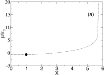
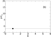
Figure 3: (a) The liquid-vapor phase boundary of the triplet-interaction kagomé lattice gas, with $\mu/\epsilon_{3}$ being a reduced chemical potential and $x=K_{3c}/K_{3}(=T/T_{c})$ a reduced temperature, where $K_{3c}(\equiv\epsilon_{3}/k_{B}T_{c})=\ln[(2+\sqrt{3})^{3}+1]=3.96992\cdots$. The curvilinear phase boundary begins at zero temperature with $\mu/\epsilon_{3}=-2/3$, and ends (analytically) at the critical point (solid circle) whose coordinates are $x=1$, $\mu/\epsilon_{3}\equiv\mu_{c}/\epsilon_{3}=-\ln(4\sqrt{3}+6)/\ln(15\sqrt{3}+27)=-0.64469\cdots$. The continuation of the phase boundary is the dashed curve which eventually diverges logarithmically at the reduced temperature $x=K_{3c}/\ln 2=5.72739\cdots$. (b) The liquid-vapor phase boundary of a conventional kagomé lattice gas having nearest-neighbor pair interactions, with $\mu/\epsilon_{2}$ being a reduced chemical potential where $\epsilon_{2}>0$ is the strength parameter of the attractive pair interaction, and $x=K_{2c}/K_{2}(=T/T_{c})$ being a reduced temperature, where $K_{2c}=\ln[(3+2\sqrt{3})]=1.86626\cdots$. The phase boundary is rectilinear, specially, the constant valued expression $\mu/\epsilon_{2}=-2$, $0\leq x\leq 1$ (solid circle locates the critical point). The continuation of the phase boundary is the horizontal dashed line which continues indefinitely.

which is nearly $50\%$ smaller than the critical value (2.10). The critical value $K_{3c}$ in (2.10) is used to locate the critical point in the relation (2.8), yielding the liquid-vapor phase boundary curve of the triplet interaction kagomé lattice gas (Figure 3a). Explicitly, one directly obtains barry

$$\mu/\epsilon_{3}=-K^{-1}_{3}\ln[(e^{K_{3}}-1)^{2/3}-1],\;\;\;0\leq K_{3c}/K_{3}\leq 1,$$ (12)

with $\mu/\epsilon_{3}$ being a reduced chemical potential and $K_{3c}/K_{3}(=T/T_{c})$ a reduced temperature where $K_{3c}(\equiv\epsilon_{3}/k_{B}T_{c})=\ln[(2+\sqrt{3})^{3}+1]=3.96992\cdots$ [(2.10)]. The curvilinear phase boundary begins at zero temperature with $\mu/\epsilon_{3}=-2/3$ and ends (analytically) at a critical point whose coordinates are $K_{3c}/K_{3}=1$, $\mu/\epsilon_{3}=\mu_{c}/\epsilon_{3}=-0.64469\cdots$. At zero temperature, the phase boundary curve $\mu/\epsilon_{3}$ vs $T/T_{c}$ has a zero slope in accordance with the Clausius-Clapeyron equation and third law of thermodynamics. Otherwise, its slope is positive which is more discernible at temperature closely below the critical temperature. As comparison, Figure 3b shows the corresponding phase diagram for the condensation of a conventional kagomé lattice gas with attractive nearest-neighbor pair interactions.

III Exact solutions for $\langle n_{0}\rangle$, $\langle n_{0}n_{1}n_{2}\rangle$ along coexistence curve of kagomé lattice gas with three-particle interactions

The coexistence surface (and boundary) of the lattice-gas system is the prominent portion of its thermal equation of state surface. More particularly, the boundary (edge) of the coexistence surface contains the critical point and encloses the liquid-vapor coexistence region (heterogeneous mixture). The projective mapping of the boundary onto the chemical potential-temperature ($\mu-T$) plane marks the previous liquid-vapor phase boundary curve (2.12), and a similar projective viewing in density-temperature ($\rho-T$) space indicates the liquid-vapor coexistence curve of the lattice gas. The latter phase diagram ($\rho^{coex}_{l,v}$ vs $T/T_{c}$) for the condensation of the triplet-interaction kagomé lattice gas has already been obtained barry . A brief review of the results is now presented for later use.

The solutions for the density $\rho(=\langle n_{0}\rangle)$ and the elementary triplet correlation $\langle n_{0}n_{1}n_{2}\rangle$ can be determined along the liquid-vapor coexistence curve and at criticality by logarithmic differentiations of the grand partition function $\Xi(\mu,\mathcal{N},T)$ [(2.7)] with respect to $\beta\mu$ and $K_{3}$, respectively, and then letting $L^{*}\rightarrow 0$ for the full range of condensation temperatures $0\leq K_{3c}/K_{3}\leq 1$. Specifically, the exact solution for the average number density $\langle n_{0}\rangle(=\rho)$ is given, as $L^{*}\rightarrow 0$, by barry

$$\rho=\begin{cases}1-\frac{1}{4}[1-(e^{K_{3}}-1)^{-2/3}][1+\langle\mu_{0}\mu_{1}\rangle_{L^{*}=0}\mp 2\langle\mu\rangle_{S}],&0\leq\frac{K_{3c}}{K_{3}}\leq 1,\\ 1-\frac{1}{4}[1-(e^{K_{3}}-1)^{-2/3}][1+\langle\mu_{0}\mu_{1}\rangle_{L^{*}=0}],&1<\frac{K_{3c}}{K_{3}}\leq\frac{K_{3c}}{\ln 2}=5.72739\cdots,\end{cases}$$ (13)

where $\langle\mu_{0}\mu_{1}\rangle_{L^{*}=0}$, $\langle\mu\rangle_{S}$ are the nearest-neighbor pair correlation and spontaneous magnetization, respectively, of the previous $S=1/2$ honeycomb Ising model ferromagnet. In the top of eq. (3.1), the $-(+)$ algebraic sign corresponds to the liquid(vapor) branch of the coexistence curve. The restricted range $\ln 2<K_{3}<\infty$ was required earlier to assure that the Ising interaction parameter $K^{*}>0$ (ferromagnetic) and leads, using (2.10), to the finite $K_{3c}/K_{3}-$ range of the temperatures in the bottom of eq. (3.1). The terminating value $K_{3c}/\ln 2=5.72739\cdots$ also guarantees that $\rho$ does not exceed $\rho_{max}=1$ corresponding to the fully occupied (“close packed”) lattice gas. The bottom expression of (3.1) is the continuation of the curvilinear diameter of the coexistence region in the top expression of (3.1) beyond the coexistence surface. In (3.1), the exact solutions for $\langle\mu_{0}\mu_{1}\rangle_{L^{*}=0}$ and $\langle\mu\rangle_{S}$ are known to be baxter ; naya

$$\langle\mu_{0}\mu_{1}\rangle_{L^{*}=0} = \frac{2}{3}[\coth 2K^{*}+\gamma K_{1}(\kappa)],$$ (14a)

$$\langle\mu\rangle_{S} = \begin{cases}(1-\kappa^{2})^{1/8},\;\;\;0\leq\frac{K^{*}_{c}}{K^{*}}\leq 1,\\ 0,\;\;\;1<\frac{K^{*}_{c}}{K^{*}}<\infty\end{cases}$$ (14b)

with $K_{1}(\kappa)$ being the complete elliptic integral of the first kind

$$K_{1}(\kappa)=\int_{0}^{\pi/2}(1-\kappa^{2}\sin^{2}\theta)^{-1/2}d\theta,$$ (15a)

and where

$$\kappa^{2} = 16z^{3}(1+z^{3})(1-z)^{-3}(1-z^{2})^{-3},$$ (15b)

$$\gamma = (1-z^{4})(z^{2}-4z+1)/\pi|1-z^{2}|(1-z)^{4},$$ (15c)

$$z = e^{-2K^{*}}.$$ (15d)

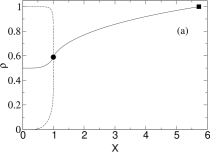
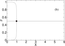
Figure 4: (a) The liquid-vapor coexistence curve of the triplet-interaction kagomé lattice gas, with $\rho$ being the particle number density and $x=K_{3c}/K_{3}(=T/T_{c})$ a reduced temperature, where $K_{3c}(\equiv\epsilon_{3}/k_{B}T_{c})=\ln[(2+\sqrt{3})^{3}+1]=3.96992\cdots$. The curvilinear diameter of the asymmetric rounded coexistence region is the solid curve which begins at zero temperature with $\rho=1/2$, and ends at the critical point (solid circle) whose coordinates are $x=1$, $\rho\equiv\rho_{c}=\frac{1}{3}(7/2-\sqrt{3})=0.58931\cdots$. The continuation of the curvilinear diameter into the disordered fluid region is the continuing sigmoidal curve which is monotonically increasing and concave downward, eventually ending at the point (solid square) with coordinates $x=K_{3c}/\ln 2=5.72739\cdots$, $\rho=\rho_{max}=1$. (b) The liquid-vapor coexistence curve of a conventional kagomé lattice gas having nearest-neighbor pair interactions, with $\rho$ being the particle number density and $x=K_{2c}/K_{2}$ being a reduced temperature where $K_{2c}=\ln[(3+2\sqrt{3})]=1.86626\cdots$. The coexistence curve is given by $\rho_{l,v}^{coex}=\frac{1}{2}(1\pm m_{s})$, where $m_{s}$ is the spontaneous magnetization of a standard kagomé Ising model. The rectilinear diameter of the symmetric rounded coexistence region is the horizontal solid line $\rho=1/2$, which ends at the critical point (solid circle) whose coordinates are $x=1$, $\rho\equiv\rho_{c}=1/2$. The continuation of the rectilinear diameter into the disordered region is the horizontal solid line which continues indefinitely.

The expressions (3.1) can be written purely in the natural $K_{3}$ notation of the lattice gas by substituting the interaction parameter relation (2.9) into (3.2) and (3.3). Then, substituting the resulting forms into the top expression of (3.1) yields the sought exact solution for the liquid-vapor coexistence curve which is plotted in Figure 4a. Additionally, the composition of the density $\rho$ at points within the two-phase coexistence region in Figure 4a can be determined by the application of the thermodynamic lever rule callen . The phase diagram of Figure 4a exhibits an asymmetric rounded shape with a curvilinear diameter, contrasting the familiar symmetric rounded shape and constant rectilinear diameter for a conventional kagomé lattice gas with attractive nearest-neighbor pair interactions (see Figure 4b). In the global comparison (i.e., “over-laying”)of Figure 4a and Figure 4b, the values of the liquid-vapor branches (and curvilinear diameter) in Figure 4a exceed the values of the liquid-vapor branches (and rectilinear diameter) in Figure 4b at all corresponding finite reduced temperatures.

The curvilinear diameter of the coexistence region in Figure 4a is the solid curve which begins at zero temperature with $\rho=1/2$, exhibits a positive slope which is more pronounced at temperatures closely below the critical temperature, and ends at the critical point (solid circle) whose coordinates are $K_{3c}/K_{3}=1$, $\rho=\rho_{c}=0.58931\cdots$ (see (3.7a)). Using the bottom expression of (3.1), the curvilinear diameter is continued beyond the coexistence region as the solid sigmoidal curve, eventually ending at the point (solid square) with coordinates $K_{3c}/K_{3}=K_{3c}/\ln 2=5.72739\cdots$, $\rho=\rho_{max}=1$.

To obtain the exact solution for the triplet correlation $\langle n_{0}n_{1}n_{2}\rangle$ along the coexistence curve, one first computes the logarithmic derivative of $\Xi(\mu,\mathcal{N},T)$ with respect to the triplet-interaction parameter $K_{3}$. Specifically, (2.7a) gives

$$\ln\Xi(\mu,{\mathcal{N}},T) = \frac{3}{4}(\frac{K_{3}}{6}+\beta\mu)\mathcal{N}^{*}+\mathcal{N}^{*}(\ln a^{*}-\ln\cosh L^{*}-\ln 2)$$ (16)

$$- \frac{3}{2}\mathcal{N}^{*}\ln\cosh K^{*}+\ln Z^{*}(L^{*},K^{*}),$$

where the total number of kagomé lattice sites $\mathcal{N}=\frac{3}{2}\mathcal{N}^{*}$ with $\mathcal{N}^{*}$ being, as stated previously, the total number of lattice sites of the associated honeycomb lattice (see Figure 2). Also, the total number of elementary triangles $\mathcal{N}_{\Delta}$ of the kagomé lattice equals $\mathcal{N}^{*}$, again seen in Figure 2. Using (2.6), (2.7) and (3.4), one obtains

$$\mathcal{N}_{\Delta}\langle n_{0}n_{1}n_{2}\rangle = \frac{\partial\ln\Xi(\mu,{\mathcal{N}},T)}{\partial K_{3}}$$ (17a)

$$= \frac{\mathcal{N}^{*}}{8}+\mathcal{N}^{*}\left[\frac{\partial\ln a^{*}}{\partial K_{3}}-(\tanh L^{*})\frac{\partial L^{*}}{\partial K_{3}}\right]$$ (17b)

$$- \frac{3}{2}\mathcal{N}^{*}(\tanh K^{*})\frac{\partial K^{*}}{\partial K_{3}}+\frac{\partial\ln Z^{*}}{\partial L^{*}}\frac{\partial L^{*}}{\partial K_{3}}+\frac{\partial\ln Z^{*}}{\partial K^{*}}\frac{\partial K^{*}}{\partial K_{3}}$$ (17c)

where

$$\frac{\partial\ln Z^{*}}{\partial L^{*}} = \mathcal{N}^{*}\langle\mu_{i}\rangle,$$ (17d)

$$\frac{\partial L^{*}}{\partial K_{3}} = \frac{1}{2}\frac{e^{K_{3}}}{e^{K_{3}}-1}\;,$$ (17e)

$$\frac{\partial K^{*}}{\partial K_{3}} = 0,$$ (17f)

$$\frac{\partial\ln a^{*}}{\partial K_{3}} = -\frac{1}{8}+\frac{e^{K_{3}}}{(e^{-\beta\mu}+1)^{3/2}+e^{K_{3}}-1}\;.$$ (17g)

Hence, as $L^{*}\rightarrow 0$, (3.5) yields

$$\langle n_{0}n_{1}n_{2}\rangle = \frac{1}{2}\frac{e^{K_{3}}}{e^{K_{3}}-1}(1\pm\langle\mu\rangle_{S}),\;\;\;\ln 2<K_{3}<\infty$$ (20)

$$= \left\{\begin{array}[]{ll}\frac{1}{2}\frac{e^{K_{3}}}{e^{K_{3}}-1}(1\pm\langle\mu\rangle_{S}),\;\;\;0\leq\frac{K_{3c}}{K_{3}}\leq 1,\\ \frac{1}{2}\frac{e^{K_{3}}}{e^{K_{3}}-1},\;\;\;1<\frac{K_{3c}}{K_{3}}\leq\frac{K_{3c}}{\ln 2}=5.72739\cdots,\end{array}\right.$$

having replaced $\langle\mu_{i}\rangle$ by $\pm\langle\mu\rangle_{s}$ in (3.5b) due to ‘spontaneous symmetry breaking’, having substituted the zero-field ($L^{*}=0$) condition (2.8) into (3.5e), used the identification $\mathcal{N}_{\Delta}=\mathcal{N}^{*}$, and having partitioned, as earlier, the (dimensionless) inverse temperature range $\ln 2<K_{3}<\infty$ into (reduced) temperature intervals below and above criticality in (3.6). Using the known result (3.2b) for the spontaneous magnetization $\langle\mu\rangle_{S}$, and substituting the interaction parameter relation (2.9) into (3.2b) and (3.3b,d), the exact solution in the upper expression of (3.6) for the elementary triplet correlation $\langle n_{0}n_{1}n_{2}\rangle$ is obtained along the coexistence curve and at criticality as a function of the (reduced) temperature $K_{3c}/K_{3}$, and is plotted in Figure 5a. Also shown in Figure 5a, the lower expression of (3.6) is the exact solution for $\langle n_{0}n_{1}n_{2}\rangle$ along the continuation of the curvilinear diameter (solid curve) beyond the coexistence surface, where the trajectory terminates at the point (solid square) with coordinates $K_{3c}/K_{3}=5.72739\cdots$, $\langle n_{0}n_{1}n_{2}\rangle=1$. The corresponding results for $\langle n_{0}n_{1}n_{2}\rangle$ in a kagomé lattice gas with attractive nearest-neighbor pair interactions are shown in Figure 5b where, as a function of temperature, the curvilinear diameter and its extension into the disordered fluid region exhibit a sigmoidal shape and monotonically decreasing behavior contrasting the results shown in Figure 5a for the three-particle interactions.

At criticality, the honeycomb Ising ferromagnet has values $\langle\mu\rangle_{S}=0$ and syozi $\langle\mu_{0}\mu_{1}\rangle_{c}=4\sqrt{3}/9$. These critical values along with the critical value (2.10) $e^{K_{3c}}=(2+\sqrt{3})^{3}+1$ are substituted into (3.1) and (3.6) yielding, respectively,

$$\rho_{c} = \frac{1}{3}(\frac{7}{2}-\sqrt{3})=0.58931\cdots,$$ (21a)

$$\langle n_{0}n_{1}n_{2}\rangle_{c} = \frac{1}{2}(\frac{27+15\sqrt{3}}{26+15\sqrt{3}})=0.50961\cdots,$$ (21b)

as critical values in the triplet-interaction kagomé lattice gas. For a traditional kagomé lattice gas with attractive nearest-neighbor pair interactions, the corresponding values are

$$\rho_{c} = \frac{1}{2}=0.50000\cdots,$$ (22a)

$$\langle n_{0}n_{1}n_{2}\rangle_{c} = \frac{1}{16}(3+2\sqrt{3})=0.40400\cdots.$$ (22b)

As seen, the one-parameter ($\epsilon_{3}$) model Hamiltonian (2.1) exhibits a single critical point on its thermal equation of state surface $\mu=\mu(\rho,T)$ (in suitable units), with critical coordinates $\mu_{c}/\epsilon_{3}=-0.64469\cdots$, $\rho_{c}=0.58931\cdots$, $k_{B}T_{c}/\epsilon_{3}\equiv K^{-1}_{3c}=0.25189\cdots$. The coexistence surface, its boundary coexistence curve and the critical point comprise the prominent portion of the above equation of state surface. The liquid and vapor branches of the coexistence curve identify at the critical point, and all lattice-gas thermal averages in the current studies are evaluated along both branches and at criticality.

Some comments are warranted on the nature of the mathematical singularities in the phase diagram of Figure 4a. The critical behaviors of the coexistence curve and the curvilinear diameter are underlaid by the known critical behaviors of the honeycomb Ising thermal averages $\langle\mu\rangle_{s}$ and $\langle\mu_{0}\mu_{1}\rangle_{L^{*}=0}$ in (3.1). Letting $\rho_{l},\rho_{v}$ denote the particle number density along the liquid and vapor branches, respectively, of the coexistence curve, the top expression in (3.1) immediately reveals that the ordering parameter $\rho_{l}-\rho_{v}$ (length of vertical “tie-line” spanning the coexistence region) realizes its critical behavior purely from $\langle\mu\rangle_{s}$, whereas the curvilinear diameter $\frac{1}{2}(\rho_{l}+\rho_{v})$ (arithmetic mean of $\rho_{l}$ and $\rho_{v}$) realizes its critical behavior solely from $\langle\mu_{0}\mu_{1}\rangle_{L^{*}=0}$. Hence, the relation (3.2b) for the Ising spontaneous magnetization $\langle\mu\rangle_{s}$ leads to the vanishing of the order parameter $\rho_{l}-\rho_{v}$ at the critical point with the Ising-type critical exponent $1/8$ (algebraic branch point singularity). Similarly, relation (3.2a) for the Ising nearest-neighbor pair correlation $\langle\mu_{0}\mu_{1}\rangle_{L^{*}=0}$ leads to the result that the curvilinear diameter $\frac{1}{2}(\rho_{l}+\rho_{v})$ and its analytic continuation into the disordered fluid region (lower expression of (3.1)) possess a weak Ising energy-type singularity mermin $\epsilon\ln\epsilon$ at the critical point, where $\epsilon>0$ is a small fractional deviation of the temperature from its critical value. In contrast, note that the constant rectilinear diameter in a conventional $d=2$ lattice gas (Figure 4b) is analytic at criticality. One also recognizes that the curvilinear diameter of the solution curve for the elementary triplet correlation $\langle n_{0}n_{1}n_{2}\rangle$ in (3.6) and Figure 5a is analytic at the critical point. In the above mathematical arguments, one uses (2.9), (2.10) and the previous literature value $K^{*}_{c}=\frac{1}{2}\ln(2+\sqrt{3})$ to establish an exact scaling relation

$$\epsilon^{*}=\frac{1}{6}\left(\frac{e^{K_{3c}}}{e^{K_{3c}}-1}\right)\frac{K_{3c}}{K^{*}_{c}}\;\epsilon=(1.02416\cdots)\epsilon$$ (23)

between the smallness parameters $\epsilon^{*}$ and $\epsilon$. The scaling relation (3.9) affords a direct proof that the singularities in the associated Ising model lead to the same nature of singularities in the lattice gas phase diagram in (3.1) and Figure 4a, viz., $\epsilon^{*1/8}\rightarrow\epsilon^{1/8}$, $\epsilon^{*}\ln\epsilon^{*}\rightarrow\epsilon\ln\epsilon$, where, neglecting second-order small quantities, $\epsilon^{*}=(K^{*}-K^{*}_{c})/K^{*}_{c}$, $\epsilon=(K_{3}-K_{3c})/K_{3c}$.

In the present section, we emphasized that the solutions for $\langle n_{0}\rangle$ and $\langle n_{0}n_{1}n_{2}\rangle$ were determined along the coexistence curve via logarithmic differentiations of the grand partition function $\Xi(\mu,{\mathcal{N}},T)$ with respect to $\beta\mu$ and $K_{3}$, respectively, and then letting $L^{*}\rightarrow 0$. To secure solutions for additional correlations, a different method is needed. In the subsequent sections, one develops and solves, as $L^{*}\rightarrow 0$, a linear algebraic system of correlation identities whose coefficients depend solely upon the interaction parameter $K_{3}$. The a priori knowledge of $\langle n_{0}\rangle$ and $\langle n_{0}n_{1}n_{2}\rangle$ will be instrumental in the quest for closure and linear independence within the linear algebraic system of identities.

IV Basic generating equation for correlation identities

The class of correlation identities currently considered is a set of linear algebraic equations with coefficients dependent only upon the interaction parameter $K_{3}$ fisher . To develop such identities systematically, one proceeds to derive their basic generating equation.

Let [g] be any function of the lattice-gas variables $n_{1},n_{2},\cdots,n_{\mathcal{N}-1}$ (excluding $n_{0}$, the origin site variable in Figure 1). Letting $H^{\prime}\equiv\mathcal{H}^{\prime}-\mu N^{\prime}$, $\sum^{\prime}_{\{n_{i}\}}$ denote a restricted energy form and summation operation, respectively, which exclude $n_{0}$, one can construct the grand canonical thermal average $\langle n_{0}[g]\rangle$ as

$$\Xi\cdot\langle n_{0}[g]\rangle = \sum_{\{n_{i}\}}\;\;n_{0}[g]e^{-\beta H}$$ (24)

$$= {\sum_{\{n_{i}\}}}^{\prime}\;\;[g]e^{-\beta H^{\prime}}\sum_{n_{0}}n_{0}e^{n_{0}[\beta\mu+K_{3}(n_{1}n_{2}+n_{3}n_{4})]}$$ (25)

$$= \sum_{\{n_{i}\}}\;\;[g]e^{-\beta H}\left[\frac{\sum_{n_{0}}n_{0}e^{n_{0}[\beta\mu+K_{3}(n_{1}n_{2}+n_{3}n_{4})]}}{\sum_{n_{0}}e^{n_{0}[\beta\mu+K_{3}(n_{1}n_{2}+n_{3}n_{4})]}}\right]$$ (26)

yielding

$$\langle n_{0}[g]\rangle=\langle\frac{e^{\beta\mu+K_{3}(n_{1}n_{2}+n_{3}n_{4})}}{1+e^{\beta\mu+K_{3}(n_{1}n_{2}+n_{3}n_{4})}}[g]\rangle,\;\;\;n_{0}\nsubseteq[g],$$ (27)

having lastly used the standard definition of grand canonical thermal average initiating (4.1). In deriving (4.1), the “split, rearrange, then reconstitute” procedures are justified since all lattice-gas variables commute. To further develop (4.2), one writes

$$\frac{e^{\beta\mu+K_{3}(n_{1}n_{2}+n_{4}n_{4})}}{1+e^{\beta\mu+K_{3}(n_{1}n_{2}+n_{3}n_{4})}}=A+B(n_{1}n_{2}+n_{3}n_{4})+Cn_{1}n_{2}n_{3}n_{4},$$ (28)

where the expansion as a finite algebraic series in the lattice-gas product variables $n_{1}n_{2}$, $n_{3}n_{4}$ reflects their idempotent nature [$(n_{p}n_{q})^{2}=n_{p}n_{q}$]. The coefficients $A$, $B$, $C$ are determined by considering the following realizations of the product variables $n_{1}n_{2},n_{3}n_{4}$ in (4.3):

• $n_{1}n_{2}=n_{3}n_{4}=0$, yielding

  $$A=\frac{e^{\beta\mu}}{1+e^{\beta\mu}}=\frac{1}{e^{-\beta\mu}+1},$$ (29a)

• $n_{1}n_{2}=0$, $n_{3}n_{4}=1$, yielding

  $$A+B=\frac{e^{\beta\mu+K_{3}}}{1+e^{\beta\mu+K_{3}}}=\frac{1}{e^{-\beta\mu-K_{3}}+1},$$ (29b)

• $n_{1}n_{2}=n_{3}n_{4}=1$, yielding

  $$A+2B+C=\frac{e^{\beta\mu+2K_{3}}}{1+e^{\beta\mu+2K_{3}}}=\frac{1}{e^{-\beta\mu-2K_{3}}+1}.$$ (29c)

The three linear algebraic inhomogeneous equations (4.4 a-c) in the three unknowns $A$, $B$, $C$ are patently linearly-independent and directly give the solutions

$$A = \frac{1}{e^{-\beta\mu}+1},$$ (30a)

$$B = \frac{1}{e^{-\beta\mu-K_{3}}+1}-\frac{1}{e^{-\beta\mu}+1},$$ (30b)

$$C = \frac{1}{e^{-\beta\mu-2K_{3}}+1}-\frac{2}{e^{-\beta\mu-K_{3}}+1}+\frac{1}{e^{-\beta\mu}+1}.$$ (30c)

For adoption along the coexistence curve, one evaluates the coefficients (4.5) at $L^{*}=0$. Substituting the (2.8) expression into (4.5), one obtains, as $L^{*}\rightarrow 0$,

$$A = (e^{K_{3}}-1)^{-2/3},$$ (31a)

$$B = e^{K_{3}}[(e^{K_{3}}-1)^{2/3}+e^{K_{3}}-1]^{-1}-(e^{K_{3}}-1)^{-2/3},$$ (31b)

$$C = e^{2K_{3}}[(e^{K_{3}}-1)^{2/3}+e^{2K_{3}}-1]^{-1}$$ (31c)

$$- 2e^{K_{3}}[(e^{K_{3}}-1)^{2/3}+e^{K_{3}}-1]^{-1}+(e^{K_{3}}-1)^{-2/3}.$$

Returning to (4.2) and substituting (4.3), the basic generating equation for multiparticle correlation identities is thus given by

$$\langle n_{0}[g]\rangle=A\langle[g]\rangle+B\langle(n_{1}n_{2}+n_{3}n_{4})[g]\rangle+C\langle n_{1}n_{2}n_{3}n_{4}[g]\rangle,\;\;\;n_{0}\nsubseteq[g],$$ (32)

where the coefficients $A$, $B$, $C$ are given by (4.6) as $L^{*}\rightarrow 0$. The linear algebraic system of correlation identities generated by (4.7) will be employed in the next section to determine the solutions for various multiparticle correlations along the coexistence curve of the triplet-interaction kagomé lattice gas.

V Exact solutions for correlations along the coexistence curve of kagomé lattice gas with three-particle interactions.

Solutions will now be determined for correlations along the coexistence curve of the present lattice gas model. More particularly, exact solutions are found for the nearest-neighbor pair and various multiparticle correlations defined upon the select nine-site cluster shown in Figure 6. In section III, pertinent exact solutions were obtained for $\langle 0\rangle$ and $\langle 012\rangle$, where, for notational simplicity, only the numeric site labels in Figure 6 are written inside the thermal average symbols. As seen shortly, the a priori knowledge of $\langle 0\rangle$ and $\langle 012\rangle$ is vital supplementary information within the system of correlation identities.

First consider the five-site (“bow-tie”) cluster $0,1,2,3,4$ (see Figure 6) and the five generators $\langle 0\rangle$, $\langle 01\rangle$, $\langle 012\rangle$, $\langle 0123\rangle$, $\langle 01234\rangle$. Employing the basic generating equation (4.7), one directly obtains the following correlation identities for $\langle 0\rangle$ and $\langle 012\rangle$, respectively,

$$\langle 0\rangle = A+B\langle 12+34\rangle+C\langle 1234\rangle,$$ (33a)

$$\langle 012\rangle = A\langle 12\rangle+B\langle 12+1234\rangle+C\langle 1234\rangle,$$ (33b)

having used the idempotent property $n^{2}_{j}=n_{j}$. The identity (5.1a) is initially the only inhomogeneous equation in the infinite system of identities. However, since $\langle 0\rangle$ and $\langle 012\rangle$ are already known along the coexistence curve, one rearranges (5.1) into the standard form of two linear algebraic inhomogeneous equations in the two unknowns $\langle 01\rangle$ and $\langle 1234\rangle$:

$$2B\langle 01\rangle+C\langle 1234\rangle = \langle 0\rangle-A,$$ (34a)

$$(A+B)\langle 01\rangle+(B+C)\langle 1234\rangle = \langle 012\rangle,$$ (34b)

where the symmetry of the kagomé lattice has been recognized in the equating of geometrically-equivalent pair correlations in (5.2). Since the LHS coefficient matrix in (5.2) has a non-vanishing determinant, equations (5.2) are linearly independent and hence determine the solutions for the nearest-neighbor pair $\langle 01\rangle$ and quartet $\langle 1234\rangle$ correlations along the coexistence curve.

Again employing the basic generating equation (4.7), the three remaining generators $\langle 01\rangle$, $\langle 0123\rangle$ and $\langle 01234\rangle$ yield, respectively, the identities

$$\langle 01\rangle = A\langle 1\rangle+B\langle 12+134\rangle+C\langle 1234\rangle,$$ (35a)

$$\langle 0123\rangle = (A+B)\langle 123\rangle+(B+C)\langle 1234\rangle,$$ (35b)

$$\langle 01234\rangle = (A+2B+C)\langle 1234\rangle.$$ (35c)

The relevant exact solutions for the thermal averages $\langle 0\rangle$, $\langle 01\rangle$, $\langle 1234\rangle$ appearing in (5.3) have already been obtained. Thus, using lattice symmetry ($\langle 1\rangle=\langle 0\rangle$, $\langle 12\rangle=\langle 01\rangle$, $\langle 134\rangle=\langle 123\rangle$), the identity(5.3a) directly determines the triplet correlation $\langle 123\rangle$, identity (5.3b) in turn directly establishes the quartet generator $\langle 0123\rangle$ since the RHS is known, and identity (5.3c) similarly secures the quintet generator $\langle 01234\rangle$ since the RHS is known. To review, exact solutions are now known along the coexistence curve for the density $\langle 0\rangle$ and six correlations defined upon the five-site (“bow tie”) cluster $0,1,2,3,4$ in Figure 6, specifically,

$$\langle 0\rangle,\langle 01\rangle,\langle 012\rangle,\langle 123\rangle,\langle 0123\rangle,\langle 1234\rangle,\langle 01234\rangle.$$ (36)

One next considers the seven-site cluster $0,1,2,3,4,5,6$ (see Figure 6) and the six generators $<03456>$, $<0456>$, $<01256>$, $\langle 012356\rangle$, $\langle 012456\rangle$, $\langle 0123456\rangle$. Using the basic generating equation (4.7), the latter generators yield, respectively, the identities

$$\langle 03456\rangle = (A+B)\langle 3456\rangle+(B+C)\langle 123456\rangle,$$ (37a)

$$\langle 0456\rangle = A\langle 456\rangle+B\langle 3456+12456\rangle+C\langle 123456\rangle,$$ (37b)

$$\langle 01256\rangle = (A+B)\langle 1256\rangle+(B+C)\langle 123456\rangle,$$ (37c)

$$\langle 012356\rangle = (A+B)\langle 12356\rangle+(B+C)\langle 123456\rangle,$$ (37d)

$$\langle 012456\rangle = (A+B)\langle 12456\rangle+(B+C)\langle 123456\rangle,$$ (37e)

$$\langle 0123456\rangle = (A+2B+C)\langle 123456\rangle.$$ (37f)

Using the lattice symmetry, some correlations in identities (5.5) on the seven-site cluster are in registry with known correlations (5.4) on the earlier five-site cluster. Specifically,

$$\langle 03456\rangle\equiv\langle 01234\rangle,\langle 3456\rangle=\langle 0456\rangle\equiv\langle 0123\rangle,\langle 456\rangle\equiv\langle 012\rangle.$$ (38)

The registry listings (5.6) are now used as a priori information in identities (5.5) thereby reducing the number of unknown correlations. Hence, in identity (5.5a), all correlations are known except the sextet correlation $\langle 123456\rangle(=\langle 012356\rangle)$, so the latter is determined. Similarly, in identity (5.5b), all correlations are now known except the quintet correlation $\langle 12456\rangle$, so the latter is obtained. In identity (5.5c), all correlations are known save the quartet correlation $\langle 1256\rangle$, so the latter is secured. Continuing the cascade reasoning, the only unknown correlation in (5.5d) is the quintet correlation $\langle 12356\rangle$ so the latter is found.In identity (5.5e), all correlations are known save the sextet generator $\langle 012456\rangle$, so the latter is determined. Lastly, in identity (5.5f), the RHS correlation is known so the LHS septet generator $\langle 0123456\rangle$ is obtained. In summary, exact solutions have been found along the coexistence curve for the additional six correlations defined upon the seven-site cluster $0,1,2,3,4,5,6$ in Figure 6:

$$\langle 1256\rangle,\langle 12356\rangle,\langle 12456\rangle,\langle 123456\rangle,\langle 012456\rangle,\langle 0123456\rangle.$$ (39)

One proceeds to consider the nine-site cluster $0,1,2,3,4,5,6,7,8$ (see Figure 6) and the six generators $\langle 0345678\rangle$, $\langle 012345678\rangle$, $\langle 05678\rangle$, $\langle 045678\rangle$, $\langle 0125678\rangle$, $\langle 01245678\rangle$. Employing again the basic generating equation (4.7), the above generators yield, respectively,

$$\langle 0345678\rangle = (A+B)\langle 345678\rangle+(B+C)\langle 12345678\rangle,$$ (40a)

$$\langle 012345678\rangle = (A+2B+C)\langle 12345678\rangle,$$ (40b)

$$\langle 05678\rangle = A\langle 5678\rangle+B\langle 125678+345678\rangle+C\langle 12345678\rangle,$$ (40c)

$$\langle 045678\rangle = A\langle 45678\rangle+B\langle 1245678+345678\rangle+C\langle 12345678\rangle,$$ (40d)

$$\langle 0125678\rangle = (A+B)\langle 125678\rangle+(B+C)\langle 12345678\rangle,$$ (40e)

$$\langle 01245678\rangle = (A+B)\langle 1245678\rangle+(B+C)\langle 12345678\rangle.$$ (40f)

Using lattice symmetry, various correlations in (5.8) on the nine-site cluster are in registry with known correlations (5.7) on the previous seven-site cluster. Specifically,

$$\langle 0345678\rangle \equiv \langle 0123456\rangle,\langle 345678\rangle\equiv\langle 012456\rangle,\langle 05678\rangle\equiv\langle 12356\rangle,$$

$$\langle 5678\rangle \equiv \langle 1256\rangle,\langle 045678\rangle\equiv\langle 123456\rangle,\langle 45678\rangle\equiv\langle 12456\rangle.$$ (41)

The registry listings (5.9) are now used as a priori information in (5.8) thus reducing the number of unknown correlations and enabling one to elicit further correlation solutions from the system of identities. In identity (5.8a), all correlations are known except the octet correlation $\langle 12345678\rangle$ so the latter is determined. Hence, the RHS of identity (5.8b) is established thereby yielding the LHS nonuplet generator $\langle 012345678\rangle$. In identity (5.8c), all correlations are known save the sextet correlation $\langle 125678\rangle$ so the latter is obtained. In identity (5.8d), all correlations are known save the septet correlation $\langle 1245678\rangle$ thus the latter is secured. In identity (5.8e), both RHS correlations are known so the LHS septet generator $\langle 0125678\rangle$ is found. Lastly, in identity (5.8f), both RHS correlations are known, hence the LHS octet generator $\langle 01245678\rangle$ is determined. In summary, exact solutions have been obtained along the coexistence curve for the additional six correlations defined upon the nine-site cluster $0,1,2,3,4,5,6,7,8$ in Figure 6:

$$\langle 125678\rangle,\langle 1245678\rangle,\langle 01245678\rangle,\langle 0125678\rangle,\langle 12345678\rangle,\langle 012345678\rangle.$$ (42)

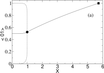
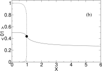
Figure 7: (a) Nearest neighbor pair correlation $\langle 01\rangle$ vs reduced temperature $x=K_{3c}/K_{3}(=T/T_{c})$ where $K_{3c}=\ln[(2+\sqrt{3})^{3}+1]=3.96992\cdots$. The solution (dashed curve) is determined along the coexistence curve including the critical point (solid circle) with coordinates $x=1$, $\langle 01\rangle_{c}=0.5239\cdots$. The solution is also secured along the continuation of the curvilinear diameter (solid curve) into the disordered region, viz., the continuing sigmoidal curve which is monotonically increasing and slightly concave downward, eventually ending at the point (solid square) with coordinates $x=K_{3c}/\ln 2=5.72739\cdots$, $\langle 01\rangle=1$. (b) Conventional pair-interaction kagomé lattice gas. Nearest-neighbor pair correlation $\langle 01\rangle$ vs reduced temperature $x=K_{2c}/K_{2}(=T/T_{c})$ where $K_{2c}=\ln[(3+2\sqrt{3})]=1.86626\cdots$. The solution (dashed curve) is determined along the coexistence curve including the critical point (solid circle) with coordinates $x=1$, $\langle 01\rangle_{c}=\frac{1}{12}(\frac{7}{2}+\sqrt{3})=0.43600\cdots$. The solution is also secured along the continuation of the curvilinear diameter (solid curve) into the disordered region, viz., the continuing sigmoidal curve which is monotonically decreasing and concave upward, eventually approaching $(\frac{1}{2})^{2}=0.25$ at infinite temperature.

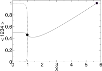
Figure 8: Quartet correlation $\langle 1234\rangle$ vs reduced temperature $x=K_{3c}/K_{3}(=T/T_{c})$ where $K_{3c}=3.96992\cdots$. The solution (dashed curve) is determined along the coexistence curve including the critical point (solid circle) with coordinates $x=1$, $\langle 1234\rangle_{c}=0.4617\cdots$. The solution is also secured along the continuation of the curvilinear diameter (solid curve) into the disordered region, viz., a concave upward curve having an asymmetric rounded minimum before monotonically increasing towards an end point (solid square) with coordinates $x=K_{3c}/\ln 2=5.72739\cdots$, $\langle 1234\rangle=1$.

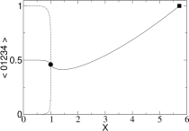
Figure 9: Quintet correlation $\langle 01234\rangle$ vs reduced temperature $x=K_{3c}/K_{3}(=T/T_{c})$ where $K_{3c}=3.96992\cdots$. The solution (dashed curve) is determined along the coexistence curve including the critical point (solid circle) with coordinates $x=1$, $\langle 01234\rangle_{c}=0.4596\cdots$. The solution is also secured along the continuation of the curvilinear diameter (solid curve) into the disordered region, viz., a concave upward curve having an asymmetric rounded minimum before monotonically increasing towards an end point (solid square) with coordinates $x=K_{3c}/\ln 2=5.72739\cdots$, $\langle 01234\rangle=1$.

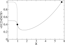
Figure 10: Nonuplet correlation $\langle 012345678\rangle$ vs reduced temperature $x=K_{3c}/K_{3}(=T/T_{c})$ where $K_{3c}=3.96992\cdots$. The solution (dashed curve) is determined along the coexistence curve including the critical point (solid circle) with coordinates $x=1$, $\langle 012345678\rangle_{c}=0.3970\cdots$. The solution is also secured along the continuation of the curvilinear diameter (solid curve) into the disordered region, viz., a concave-upward curve having an asymmetric rounded minimum before monotonically increasing towards an end point (solid square) with coordinates $x=K_{3c}/\ln 2=5.72739\cdots$, $\langle 012345678\rangle=1$.

To review, one considered correlations defined upon the nine-site cluster (Figure 6) of the kagomé lattice comprising a central triangle with its three corner-sharing triangles. The collective contents of (5.4), (5.7) and (5.10) reveal that exact solutions have been found for the density $\langle 0\rangle$, nearest-neighbor pair correlation $\langle 01\rangle$, and seventeen multiparticle correlations, all along the coexistence curve and at criticality, of the triplet-interaction kagomé lattice gas. Also, the solution for each thermal average was determined along a finite-length critical isofield ($L^{*}=0$) trajectory in the disordered fluid region of $\rho-T$ space. In this context, illustrative correlations $\langle 01\rangle$, $\langle 1234\rangle$, $\langle 01234\rangle$, $\langle 012345678\rangle$ are each plotted as functions of the reduced temperature $x=K_{3c}/K_{3}(=T/T_{c})$ in Figures 7a,8,9,10, respectively. Along the coexistence curve (Figure 4a), each correlation solution exhibits an asymmetric rounded shape with an infinite slope at the critical point (solid circle). The degree of asymmetry is associated with the slope of the curvilinear diameter in the graph, which is more pronounced at temperatures closely below the critical temperature ($x=1$). One observes that the slope is positive for the elementary triplet and nearest-neighbor pair correlations in Figures 5a and 7a, respectively, and negative for the quartet, quintet and nonuplet correlations in Figures 8, 9 and 10, respectively. A positive (negative) slope of the curvilinear diameter implies that the correlation solution curve along the upper liquid branch falls slower (faster) than the corresponding rise of the solution curve along the lower vapor branch. In each case of negative slope of the curvilinear diameter (Figures 8, 9, 10), the correlation solution along the continuation of the curvilinear diameter into the disordered region shows a rounded minimum before ascending to the common maximum value (solid square) associated with the fully occupied lattice.

VI Example of Application

A simple example employing multiparticle correlations occurs in cavitation theory brennen . One seeks the probability of an elementary cavity or void in the fluid system, where an elementary cavity is construed to be an empty site with all its nearest-neighbor sites occupied. In a kagomé lattice gas, the joint probability $p_{0,1,1,1,1}$ that the origin site 0 is empty and its four nearest-neighbor sites $1,2,3,4$ are occupied equals the thermal average value $\langle(1-n_{0})n_{1}n_{2}n_{3}n_{4}\rangle$. This probabilistic interpretation of the thermal average can be directly extracted from the standard definition of average value in probability theory, as will now be shown.

Let $f(n_{0},n_{1}...,n_{4})$ be a function of the lattice-gas discrete random variables $n_{0},n_{1},...,n_{4}$ (see “bow-tie” cluster in Figure 1). Then, the average value $\langle f(n_{0},n_{1},...,n_{4})\rangle$ is defined by

$$\langle f(n_{0},n_{1},...n_{4})\rangle=\sum_{\{n_{0},n_{1},...,n_{4}\}}p_{n_{0},n_{1},...,n_{4}}f(n_{0},n_{1},...,n_{4}),$$ (43)

where $p_{n_{0},n_{1},...,n_{4}}$ is the joint probability of a specific realization of the variables $n_{0},n_{1},...,n_{4}$ and the summation symbol $\{n_{0},n_{1},...,n_{4}\}$ represents the set of all possible $2^{5}=32$ realizations of the five lattice gas variables.

Considering a select function

$$f(n_{0},n_{1},...,n_{4})=(1-n_{0})n_{1}n_{2}n_{3}n_{4},$$ (44)

the definition (43) immediately “filters out” the desired result

$$\langle(1-n_{0})n_{1}n_{2}n_{3}n_{4}\rangle=p_{0,1,1,1,1},$$ (45)

since the value of $f(0,1,1,1,1)=1$ and all other values of the function (44) vanish in the weighted summation (43). This completes the proof.

It is instructive to mention that taking thermal averages of select operator functions is a direct and general method for exactly structuring the elements of reduced statistical density matrices note2 in equilibrium statistical mechanics. Each diagonal element of a reduced statistical density matrix is a thermal average value having a familiar probabilistic interpretation similar to (45).

Expanding (45), the probability $p_{0,1,1,1,1}(\equiv p)$ of an elementary cavity becomes the difference

$$p=\langle n_{1}n_{2}n_{3}n_{4}\rangle-\langle n_{0}n_{1}n_{2}n_{3}n_{4}\rangle.$$ (46)

The representation (46) is valid for arbitrary lattice gas interactions (pair, triplet, …) upon any four-coordinated regular lattice, i.e., the $d=2$ square and kagomé lattices and the $d=3$ diamond lattice. In Section V, exact solutions for both RHS correlations in (46) were obtained along the coexistence curve and at the critical point of the triplet-interaction kagomé lattice gas. Consequently, the probability $p$ in (46) is likewise determined along the coexistence curve and at criticality, as well as along the finite-length critical isofield ($L^{*}=0$) curve in the disordered fluid region of $\rho-T$ space. In this setting, the RHS difference of correlations in (6.4) is seen as the graphical subtraction of Figure 9 from Figure 8.

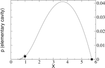
Figure 11: Probability $p$ of an elementary cavity vs reduced temperature $x=K_{3c}/K_{3}(=T/T_{c})$ where $K_{3c}=3.96992\cdots$. The solution (dashed curve) is determined along the coexistence curve including the critical point (solid circle) with coordinates $x=1$, $p_{c}=\langle 1234\rangle_{c}-\langle 01234\rangle_{c}=0.0021\cdots$. The solution is also secured along the continuation of the curvilinear diameter (solid curve) into the disordered region, viz., a concave-downward curve with a symmetric rounded maximum located at $\tilde{x}=3.6\cdots$, $p=0.0409\cdots$, before monotonically decreasing towards a nodal end point (solid square) at $x=K_{3c}/\ln 2=5.72739\cdots$ (fully occupied lattice).

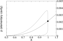
Figure 12: Enlargement of Fig 11 in the range of (reduced) condensation temperatures $0\leq x\leq 1$. Along the upper liquid branch $\rho_{l}$ of the coexistence curve, the probability $p$ of an elementary cavity attains an asymmetric rounded maximum located at $x=0.98\cdots$, $p=0.0036\cdots$. The solid circle is the critical point with coordinates $x=1$, $p_{c}=0.0021\cdots$.

The results, viz., $p$ vs $x$, are exhibited in Figure 11 and Figure 12, the latter being an enlargement of the former in the range of (reduced) condensation temperatures $0\leq x\leq 1$. At absolute zero temperature, the coexistence curve $\rho$ vs $x$ in Figure 4a is unity (zero) for the liquid (vapor) branch. In either case (fully occupied or completely empty lattice), an elementary cavity cannot exist, so $p$ vanishes at zero temperature in Figure 11 (or 12). For increasing temperatures in Figure 12, the probability $p$ of an elementary cavity along the liquid branch increasingly exceeds that along the vapor branch, except at temperatures closely below the critical temperature ($x=1$) where the two branches become identical. Such asymmetric behavior is physically anticipated since decreasing the particle number density $\rho_{l}$ along the liquid branch, beginning from a fully-occupied ground state liquid phase, creates increasingly more elementary cavities than increasing $\rho_{v}$ along the vapor branch, beginning from a completely empty ground state vapor phase. Furthermore, the curve $p$ vs $x$ in the disordered region ($x>1$) of Figure 11 exhibits a rounded maximum $p_{max}=0.0409\cdots$ at $x=\tilde{x}=3.6\cdots$, and eventually vanishes at $x=5.72739\cdots$ corresponding to $\rho=\rho_{max}=1$ (fully occupied lattice) in Figure 4a. The latter node of $p$ along the critical isofield ($L^{*}=0$) trajectory is deemed to be a multiparticle interaction effect. In Figure 11, the above maximum value $p_{max}$ is larger by an order of magnitude than the lower temperature ($x=0.98\cdots$) maximum value along the liquid branch of the coexistence curve. A synoptic view of Figures 4a, 11 and 12 enables one to numerically eliminate their common temperature variable $x$ and obtain the graph $p$ vs $\rho$.  In particular, the probability value $p_{max}=0.0409\cdots$ corresponds to a density value $\rho=\tilde{\rho}=0.88\cdots$, and $p$ monotonically increases (decreases) for the density range $\rho_{c}<\rho<\tilde{\rho}(\tilde{\rho}<\rho\leq 1)$, where $\rho_{c}=0.58931\cdots$ [(3.7a)].

Reflecting upon the traditional case of attractive nearest-neighbor pair interactions in a kagomé lattice gas, the critical isofield ($L^{*}=0$) solution for $\rho$ in the disordered region of Figure 4b is a constant at all temperatures, i.e., $1<x<\infty$, $\rho=\frac{1}{2}$ (half-filled lattice). The half-filled condition infers that the probability $p$ of an elementary cavity is non-vanishing along the critical density ($\rho_{c}=\frac{1}{2}$) line at all temperatures $1<x<\infty$ in Figure 4b. For instance, as the (reduced) temperature $x\rightarrow\infty$, $p\rightarrow\left(\frac{1}{2}\right)^{4}-\left(\frac{1}{2}\right)^{5}=\frac{1}{32}=0.03125$, having used (46) with the realization therein that the average of a product equals the product of the averages at infinite temperature. The absence of a node in the solution curve $p$ vs $x$ for pair interactions at all temperatures $1<x<\infty$ lends credence to the earlier contention that the finite-temperature node in Figure 11 for triplet interactions is a multiparticle interaction effect.

VII Summary and discussion

Exact results in physics are valuable for a variety of reasons. Endeavoring to retain only the most essential ingredients of a physical problem, exact solutions of simple model systems often provide definite guidance and insights on more realistic and invariably more mathematically complex systems. Exact results in tractable models of seemingly different physical systems may alert researchers to significant common features of these systems and actually emphasize concepts of universality. In addition to their own aesthetic appeal, exact results can, of course, serve as standards against which both approximation methods and approximate results may be appraised. Also, the underlying mathematical structures of exactly soluble models in statistical physics are rich in content and have led to important developments in mathematics.

Phase diagrams for the condensation of a two-dimensional (d=2) kagomé lattice gas with purely three-particle interactions were determined previously barry . Specifically, the liquid-vapor phase boundary (chemical potential vs temperature) and the companion liquid-vapor coexistence curve (density vs temperature) were obtained. These exact phase diagrams were briefly reviewed in the present paper to make it self-contained and for later key use in securing solutions for multiparticle correlations along the coexistence curve and at the critical point of the triplet-interaction kagomé lattice gas. Pertinent exact solutions for the average particle-number density $\langle n_{0}\rangle$ and the elementary triplet correlation $\langle n_{0}n_{1}n_{2}\rangle$ of the lattice gas were obtained via direct logarithmic differentiations of the grand canonical partition function with respect to the (dimensionless) variables $\beta\mu$ and $K_{3}$, respectively, and then taking an appropriate vanishing field limit ($L^{*}\rightarrow 0$). However, to establish solutions for additional correlations upon the coexistence curve, a different method was necessary. The method required supplemental use of the known solutions for $\langle n_{0}\rangle$ and $\langle n_{0}n_{1}n_{2}\rangle$, and is briefly discussed below.

A linear algebraic system of correlation identities was generated having coefficients dependent solely upon the interaction parameter $K_{3}$ when evaluated along the coexistence curve. Using the previously determined solutions for $\langle n_{0}\rangle$ and $\langle n_{0}n_{1}n_{2}\rangle$ as a priori information, one succeeded in finding a closed and linearly independent set of correlation identities defined upon a spatially compact nine-site cluster (Figure 6) of the kagomé lattice. Employing simple algebraic techniques, exact solutions are thereby now known for the density $\langle n_{0}\rangle$, the nearest-neighbor pair correlation $\langle n_{0}n_{1}\rangle$ and seventeen multiparticle correlations, all along the coexistence curve and at criticality of the triplet interaction kagomé lattice gas. The correlation solutions were also secured along the continuation of the curvilinear diameter of the coexistence region into the disordered fluid region of $\rho-T$ space. To our knowledge, these are the first examples, certainly away from criticality, of exact solutions for multiparticle correlations in any planar lattice-statistical model with multiparticle interactions. Along the coexistence curve (Figure 4a), the graphs of various correlation solutions were plotted (Figures 5a, 7a, 8, 9, 10) as functions of the temperature, and each solution curve exhibited an asymmetric rounded shape with an infinite slope at the critical point (solid circle). The degree of asymmetry was associated with the slope of the curvilinear diameter in the graph, and a negative slope (Figures 8, 9, 10) was a harbinger for the correlation solution to have a rounded minimum along the continuation of the curvilinear diameter into the disordered region. The exact solution curves were compared with the corresponding results in a conventional half-filled kagomé lattice gas having nearest-neighbor pair interactions, and the solutions for the multiparticle correlations were applied to cavitation theory in the condensation of the lattice gas.

The class of correlation identities currently considered has appeared in the literature fisher for almost five decades, particularly in the context of planar Ising models with nearest-neighbor pair interactions. In the present paper, however, the correlation identities were developed within the framework of the grand canonical ensemble for a kagomé lattice gas having localized three-particle interactions. As reviewed above, solutions were determined for various localized correlations of the lattice gas. One further reasons that the lengths of the vertical “tie-lines” connecting the upper and lower branches of the solution curves vanish with an Ising-type critical exponent $1/8$, and the curvilinear diameter of each solution curve is either analytic at the critical point or possesses a weak Ising energy-type singularity $\epsilon\ln\epsilon$. Supporting arguments for these asserted behaviors involve the following particulars. The critical behaviors of the lattice gas model are embedded in the system of identities at the outset, entering the initial identities (5.2a,b) via substitution of known solutions for $\langle n_{0}\rangle$, $\langle n_{0}n_{1}n_{2}\rangle$ into the inhomogeneous terms. The remaining identities (5.3), (5.5) and (5.8) are homogeneous relations among correlations. Solutions for seventeen correlations are then directly determined by elementary linear algebraic procedures and cascade orderings within the system of identities. Aside from well-behaved additive terms containing solely coefficients (4.6), all solutions can eventually be represented as linear combinations of $\langle n_{0}\rangle$ and $\langle n_{0}n_{1}n_{2}\rangle$. Hence, one concludes that the familiar Ising-type critical singularities $\epsilon^{1/8}$, $\epsilon\ln\epsilon$ inherent in $\langle n_{0}\rangle$ and $\langle n_{0}n_{1}n_{2}\rangle$ similarly characterize the singular behaviors in the subsequent seventeen correlation solutions.

Extensions in these results for the number of correlation solutions and the shapes and sizes of the $n$-site clusters could be aided by computer search codes in linear algebra theory. In these searches, one anticipates linear independence in a system of identities to be a more elusive algebraic property than closure. Finally, if one assumes a “clustering property” (asymptotic separability) for the correlations in the model, one can then employ the present known solutions for correlations on smaller length scales to gain information on chosen asymptotically long-distance-type correlations. A simple example reifies these concepts. Let $q_{1},q_{2};$ $r_{1},r_{2},r_{3};$ $s_{1},s_{2},s_{3},s_{4},s_{5}$ be the lattice sites of a nearest-neighbor bond, an elementary triangle and a “bow-tie” configuration, respectively, where the $q-$, $r-$, $s-$clusters of sites are mutually separated by asymptotically large distances. Then, the “clustering property” yields the decuplet correlation

$$\langle n_{q_{1}}n_{q_{2}}n_{r_{1}}n_{r_{2}}n_{r_{3}}n_{s_{1}}n_{s_{2}}n_{s_{3}}n_{s_{4}}n_{s_{5}}\rangle\sim\langle 01\rangle\langle 012\rangle\langle 01234\rangle,$$ (47)

having lastly used lattice symmetry and earlier notations. The result (7.1) shows that the chosen decuplet correlation asymptotically equals the graphical multiplication of the solution curves in Figures 5a, 7a and 9.

Figure 1: The kagomé lattice is a two-dimensional periodic array of equilateral triangles and regular hexagons. The lattice is regular (all sites equivalent, all bonds equivalent) and has coordination number 4. The origin site and its four nearest neighboring sites are specifically enumerated. Whenever three atoms of the lattice gas simultaneously occupy the vertices of an elementary triangle (say sites $0,1,2$), these atoms experience a triplet interaction with strength parameter $\epsilon_{3}$.

Figure 2: A honeycomb lattice (dashed bonds) may be associated with the kagomé lattice (solid bonds). A honeycomb lattice (dashed bonds) is a two-dimensional periodic array of regular hexagons, is regular (all sites equivalent, all bonds equivalent) and has coordination number 3. The origin site and its three nearest-neighboring sites are specifically enumerated upon the associated honeycomb lattice.

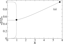
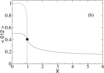
Figure 5: (a) Elementary triplet correlation $\langle 012\rangle$ vs reduced temperature $x=K_{3c}/K_{3}(=T/T_{c})$, where $K_{3c}=3.96992\cdots$. The solution (dashed curve) is determined along the coexistence curve including the critical point (solid circle) with coordinates $x=1$, $\langle 012\rangle_{c}=\frac{1}{2}(27+15\sqrt{3})/(26+15\sqrt{3})=0.50961\cdots$. The solution is also secured along the continuation of the curvilinear diameter (solid curve) into the disordered region, viz., the monotonically increasing and concave-upward curve, eventually ending at the point (solid square) with coordinates $x=K_{3c}/\ln 2=5.72739\cdots$, $\langle 012\rangle=1$. (b) Conventional pair-interaction kagomé lattice gas. Elementary triplet correlation $\langle 012\rangle$ vs reduced temperature $x=K_{2c}/K_{2}$ where $K_{2c}=1.86626\cdots$. The solution (dashed curve) is determined along the coexistence curve including the critical point (solid circle) with coordinates $x=1$, $\langle 012\rangle_{c}=\frac{1}{16}(3+2\sqrt{3})=0.40400\cdots$. The solution is also secured along the continuation of the curvilinear diameter (solid curve) into the disordered region, viz., the continuing sigmoidal curve which is monotonically decreasing and concave upward, eventually approaching $(\frac{1}{2})^{3}=0.125$ at infinite temperature.

Figure 6: Nine sites of the kagomé lattice are specifically enumerated for selected applications of the theory.

References

- (1) R.K. Ghosh and R.E. Shrock, Phys. Rev. B 30, 3790 (1984); R.E. Shrock and R.K. Ghosh, Phys. Rev. B 31, 1486 (1985).
- (2) E.W. Montroll, R.B. Potts and J.C. Ward, J. Math. Phys. 4, 308 (1963); P.W. Kasteleyn, in Graph Theory and Theoretical Physics, edited by F. Harary (Academic, London 1967); J. Stephenson, J. Math. Phys. 5, 1009 (1964); 7, 1123 (1966); 11, 413 (1970); 11, 420 (1970); T.C Choy, J. Math. Phys. 25, 3558 (1984); J.H. Barry, M. Khatun and T. Tanaka, Phys. Rev B 37, 5193 (1988); R.J. Baxter and T.C. Choy, Proc. R. Soc. London Ser A 423, 279 (1989); J.H. Barry, T. Tanaka, M. Khatun and C.H. Múnera, Phys. Rev B 44, 2595 (1991), and references cited therein.
- (3) B.M. McCoy and T.T. Wu, The Two-Dimensional Ising Model (Harvard University, Cambridge, Massachusetts, 1973); R.J. Baxter, Exactly Solved Models in Statistical Mechanics, (Academic, London, 1982).
- (4) The Ising model is one of the most studied models in theoretical and computational physics with a broad variety of applications. A valuable cumulative index for theoretical investigations upon the model and for its applications is: Phase Transitions and Critical Phenomena, Vol 20, Eds. C. Domb and J.L. Lebowitz (Academic, New York 2001); C. Domb, The Critical Point, (Taylor and Francis, London 1996). See also A. Pelissetto and E. Vicari, Phys. Rep. 368, 549 (2002).
- (5) M.E. Fisher, J. Math. Phys. 4, 124 (1963); M.F. Thorpe and A.R. McGurn, Phys. Rev. B 20, 2142 (1979); R. Schäfer, H. Beck and H. Thomas, Z. Phys. B 41, 259 (1981).
- (6) G.D. Mahan, Phys. Rev. B 14, 780 (1976); N.L. Sharma and T. Tanaka, Phys. Rev. B 28, 2146 (1983); T. Tanaka, M.A. Sawtarie, J.H. Barry, N.L. Sharma and C.H. Múnera, Phys. Rev. B 34, 3773 (1986).
- (7) M.E. Fisher, ref. fisher1 ; J. Stephenson, J. Math. Phys. 5, 1009 (1964); J.H. Barry and M. Khatun, Phys. Rev. B 35, 8601 (1987).
- (8) G.A.T. Allan and D.D. Betts, Can. J. Phys. 46, 799 (1968); M. Thomsen, M.F. Thorpe, T.C. Choy and D. Sherrington, Phys. Rev. B 30, 250 (1984); S.W. Lovesey, Theory of Neutron Scattering from Condensed Matter, (Clarendon, Oxford, 1984); J.H. Barry and S.E. Nagler, J. Phys. Condens. Matter 3, 3959 (1991).
- (9) J.W. Essam in Phase Transitions and Critical Phenomena, Vol. 2, Eds. C. Domb and M.S. Green (Academic, New York, 1973).
- (10) F. Verstraete, M. Popp and J.I. Cirac, Phys. Rev. Lett. 92, 027901 (2004).
- (11) C.E. Brennen, Cavitation and Bubble Dynamics, (Oxford University, Oxford, 1995); S. Putterman, P.G Evans, G. Vazquez and K. Weninger, Nature (London) 409, 782 (2001); M.P. Brenner, S. Hilgenfeldt and D. Lohse, Rev. Mod. Phys. 74, 425 (2002).
- (12) Models having multiparticle or multispin interactions are found, e.g., in the areas of lattice gauge theories: J. Kogut and L. Susskind, Phys. Rev. D 11, 395 (1975); binary alloys: D. F. Styer, M.K. Phani and J.L. Lebowitz, Phys. Rev. B 34, 3361 (1986); lipid bilayers: H.L. Scott, Phys. Rev. A 37, 263 (1988); magnetic excitations in cuprate two-leg ladder systems: K.P. Schmidt and G.S. Uhrig, Mod. Phys. Lett. B 19, 1179 (2005).
- (13) J.H. Barry and N.S. Sullivan, Int. J. Mod. Phys. B 7, 2831 (1993). A direct mapping also exists between the phase diagrams of the present lattice gas model and the magnetic phase diagrams of a three-parameter kagomé Ising model. See J.H. Barry and K.A. Muttalib, Physica A 311, 507 (2002).
- (14) F.Y. Wu, J. Math. Phys. 15, 687 (1974).
- (15) X.N. Wu and F.Y. Wu, J. Stat. Phys. 50, 41 (1988); J. Phys. A 22, L55, L1031 (1989); F.Y. Wu and X.N. Wu, Phys. Rev. Lett. 63, 465 (1989).
- (16) K.Y. Lin and B.H. Chen, Int. J. Mod. Phys. B 4, 123 (1990).
- (17) F.Y. Wu, J. Phys. A 23, 375 (1990).
- (18) R.B. Griffiths, in Phase Transitions and Critical Phenomena, Vol 1, eds. C. Domb and M.S. Green (Academic, New York, 1972).
- (19) R. J. Baxter and I.G. Enting, J. Phys. A 11, 2463 (1978); R.J. Baxter, ref. 2; also see R.M.F. Houtappel, Physica 16, 425 (1960).
- (20) S. Naya, Prog. Theor. Phys. 11, 53 (1954); I. Syozi in Phase Transitions and Critical Phenomena, Vol 1, eds. C. Domb and M.S. Green (Academic, New York, 1972); J.H Barry et al, ref. 2.
- (21) See, e.g., H.B. Callen, Thermodynamics, (John Wiley, New York, 1960).
- (22) I. Syozi, ref. 20.
- (23) N.D. Mermin and J. Rehr, Phys. Rev. Lett. 26, 1155 (1971); Phys. Rev. A 8, 472 (1973).
- (24) M.E. Fisher, Phys. Rev. 113, 969 (1959); R. Dekeyser and J. Rogiers, Physica 59, 23 (1972); M. Suzuki, Phys. Lett. 19, 267 (1965); Int. J. Mod. Phys. B 16, 1749 (2002); J.H Barry et al, ref. 2; T. Tanaka, ref. 25.
- (25) Theory and application for exactly-structured reduced statistical density matrices are found in the cluster-variation method of equilibrium statistical mechanics. See T. Tanaka, Methods of Statistical Physics (Cambridge University Press, United Kingdom, 2002).