Boom and bust in continuous time evolving economic model

Abstract

We show that a simple model of a spatially resolved evolving economic system, which has a steady state under simultaneous updating, shows stable oscillations in price when updated asynchronously. The oscillations arise from a gradual decline of the mean price due to competition among sellers competing for the same resource. This lowers profitability and hence population but is followed by a sharp rise as speculative sellers invade the large un-inhabited areas. This cycle then begins again.

1 Introduction

Cycles in natural and economic systems are widely observed and are often described by analogy to the differential equations describing physical oscillating systems. However, the observed oscillations are frequently irregular. In some cases, such as the Milankovitch cycles which drive ice ages, this irregularity may be an interplay between different deterministic modes (precession, obliquity and eccentricity), however the possibility of stochastic effects producing low frequency oscillations has been widely overlooked.

In economics, Schumpeter’s equilibrium theories related business cycles to oscillations about equilibrium in a dynamical system. Other authors relate cycles to time lags in the system: the cobweb model Kaldor:1934 in which price is determined by supply, which is in turn determined by previous prices; or Kitchin’s inventory model which has prices determined by stored goods Kitchin:1923 . See also the macroeconomic models of Lucas Lucas:1975 and Blinder Blinder:1981 . Further authors have proposed bubbles of overconfidence (e.g. Elliot Frost:1995 , Juglar) or external controlling influences (as, for example, governmental policy changes) as the driving force behind business cycles. Finally, Kondratieff’s long wave cycle Kondratieff:1935 has cycles driven by exogenous innovation shocks. We might imagine that these should be irregularly spaced and stochastic in nature, they are not however treated as such. This is in part because the measured quantities (various economic indicators) are seen as separate from the underlying driving forcer.

In ecological systems, the model of Lotka-Volterra gives regular oscillations, while more recent food-web and evolutionary models Bak:1993 ; Laird:2007 tend to have stable epochs punctuated by rapid change in the spirit of the punctuated equilibrium of Eldredge and Gould Eldredge:1972 ; Gould:1977 . Regular oscillations driven by lags in reacting to a change in environment are also observed Bascompte:1997 (in a similar manner to the above-mentioned economic models).

2 A simple marketplace model

In a previous paper, we introduced a simplified model of a market subject to none of these drivers, rather relying on supply-led competition and evolution through bankruptcy and startups Mitchell:2007 . Competition occurs through price – low prices increase the chance of sales, but reduce the profit margin. A dual ecological model considers competition for resources – effective foraging requires a high metabolic rate and a need to eat more frequently. In this paper we will use the language of the economic model.

Here we consider a continuous time version of the model, and show that it generates spontaneous oscillations of irregular period.

The details of the model are as in previous work Mitchell:2007 except for the choice of update scheme. We consider a ring of $2N$ alternating sellers and buyers ($N$ of each), the lattice layout showing connections is shown in Fig. 1.

Figure 1: Diagram showing lattice of buyer-seller interactions. Sellers are marked as squares, buyers as circles.

Each seller has capital $C_{i}$ and fixed price $P_{i}$ ($i=1,\dots,N$). Initial prices are drawn from $P_{i}\in[0,P_{\textrm{max}})$, and initial capital is $C_{i}=0\;\forall i$. A timestep consists of N iterations of the following:

1. One seller ($j$) is chosen uniformly at random and pays overhead $d=2$, decreasing the capital $C_{j}$ by 2.

2. One buyer ($i$) is chosen uniformly at random and the lower priced of the two adjacent seller sites ($k=j\textrm{ or }j+1$) increases its capital $C_{k}$ by $P_{k}$.

Hence in each timestep, on average, each buyer makes one purchase and each seller pays one overhead.

Sellers which have not paid an overhead still have the ability to produce goods for a buyer: we treat the overhead as a fixed cost, rather than a payment for the acquisition of goods to sell. At the end of the timestep, we now remove bankrupt sellers in the following manner:

1. All sellers with $C_{i}<0$ are bankrupt: site $i$ becomes vacant.

2. Vacant sites are repopulated with probability $\gamma$.

3. New sellers at site $i$ have $C_{i}=0$ (writing off any debt the previous seller may have had).

4. New sellers at site $i$ take the price of a randomly chosen existing site $j$, $P_{i}=P_{j}+dp$, ($dp\in[-\min(\Delta,P_{j}),\Delta]$).

This completes one complete timestep for the model. Note that the buyer sites are always occupied but seller sites may be vacant: in some rounds, some buyers have no choice of supplier. The only two free parameters in the model are $\gamma$ and $\Delta$.

It is worth mentioning that the seller dynamics mean that sellers have neither rational expectations of the market, nor any explicit memory of past transactions: implicitly the market behaviour is encoded in the time evolution of seller capital, this is however not consulted when choosing a strategy except for the case of bankruptcy when $C(t-1)>0$ and $C(t)<0$ when the strategy of the seller changes. The hold-over of capital by sellers is similar to a model of Lucas Lucas:1975 in which it is found that exogenous unanticipated shocks to a collection of independent markets (Phelpsian Islands) can have the effect (if there is memory causing information lags) of producing cyclical output. In our model there are no external shocks, the variations in the market being driven solely by the internal dynamics.

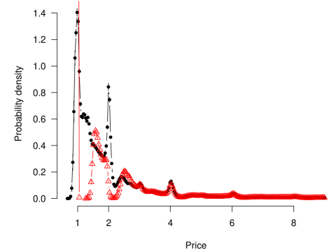
For high values of the rebirth parameter $\gamma$, only sellers charging close to their marginal cost can survive, however for $\gamma\lessapprox 0.5$ the price distribution formed favoured peaks Mitchell:2007 at higher prices. We will refer to sellers with $P_{i}\approx 1$, $\langle C_{i}\rangle\approx 0$ as ‘cheap’ and those with sufficiently high price to accumulate capital $\langle C_{i}\rangle>1$ ‘expensive’. We find that expensive sellers are still present in the continuous time formulation as shown in Fig. 2.

Figure 2: Comparison of steady state price distribution for continuous (black, circles) and discrete (red, triangles) time simulations with $N=10^{6}$, $\Delta=0.04$, $\gamma=0.5$. Error bars show standard error in the mean for 20 time-averaged distributions sampled 1000 timesteps apart after steady state is reached. Note that for the continuous time model, there is no fixed break even price, although on average $P=1$ is break even. High prices cut off at $P=9$ for clarity, along with the discrete time peak at $p=1$ which reaches 12.

Note that unlike many microscopic models Shnerb:2000 ; Guan:2006 ; Nowak:1994 of evolutionary competition, the favouring of certain strategies is not enhanced by niche construction for similar organisms. Rather, sellers are only able to construct niches which enhance the selection of competitor strategies. Expensive sites do not survive by conferring an advantage on similar expensive sites (the cheap sellers have a much higher fitness when invading): niches for expensive sellers exist in gaps between cheap sites Mitchell:2007 .

3 Oscillatory behaviour

As $\gamma$ is increased above $\approx 0.5$, the system enters an oscillatory state after an early time transient decay (erasing the initial conditions). The phase diagram (Fig. 3 insert) shows schematically the region in parameter space which leads to such a situation. These oscillations are evident as a slow decrease followed by a fast increase in the total number of sellers and the mean price of the system. This boom-bust cycle is stable across many oscillatory periods and is occasionally interspersed with larger excursions.

This regime is not seen in the discrete time model Mitchell:2007 since the high-priced sellers are not able to persist in unfavourable situations. Stochastic dynamics can however allow their persistence, since it is not a given that an expensive seller will have to pay overhead during a round in which it is not selling. This is enough to persist long-lived expensive sellers, which as we shall see drive the oscillations.

Figure 3: Ensemble-averaged unsatisfied demand (fraction of unsold to buyers) as a function of birth-rate, $\gamma$, in an enforced Bertrand steady state (open circles, error bars too small to show) and unrestricted steady state (solid circles), $N=10^{4}$, $\Delta=0.04$. Error bars show standard error in the mean over thirty ensembles after steady state is reached. In contrast to the discrete time version, the Bertrand solution diverges from unrestricted result at $\gamma\approx 0.8$ (c.f. Mitchell:2007 where the two are identical until $\gamma\approx 0.6$). This intermediate regime ($0.5\lessapprox\gamma\lessapprox 0.8$) is the region of oscillatory behaviour. Inset shows a schematic phase diagram with the three regions marked, dotted line shows position of in phase space of unsatisfied demand data.

3.1 Aperiodicity

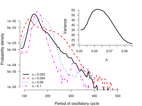
Unlike other models of boom-bust cycles (see for example Mullineux:1993 for a review), we find that the period of the oscillations is not a simple function of the model parameters, instead, the period is stochastic in nature with a typical length (Fig. 4), the origin of this stochasticity is explained in greater detail below. The shape of the distribution takes broadly two forms, for ‘small’ $\Delta$ the peak is Gaussian with a heavier, exponential right tail of high prices. For ‘large’ $\Delta$ more of the probability mass is in the peak with a less pronounced right tail. These differences may be explained by considering the exact character of the oscillations. When $\Delta$ is small ($\Delta\lessapprox 0.05$) the range of prices that the oscillations cover is typically also small $0.6<\bar{P}<1.3$ with intermittent larger excursions to $\bar{P}\approx 2$. For larger $\Delta\gtrapprox 0.07$, the typical oscillation is over a wider range of price $0.08<\bar{P}<2$ with fewer large or small excursions. The modal period of these differing regimes is approximately the same as $\Delta$ also influences the rate of change of $\bar{P}$. This compensates to some extent for the larger change required in $\bar{P}$ to complete a period. The cross-over between the two regimes is gradual which may be seen by considering the variance of the period distribution as a function of $\Delta$ (Fig. 4 inset).

Figure 4: Distribution of cycle period lengths for different values of $\Delta$ as indicated in legend, $N=10^{4}$, $\gamma=0.7$. Data prepared by smoothing time-series for the number of live sellers with a 40-point moving average to remove high-frequency components and then calculating the distance between zeroes of the derivative of the dataset. The peak and left tail are well-fitted by Normal distributions while the right tail is heavier (with an approximate exponential decay). Inset shows how the variance of the distribution varies with $\Delta$.

4 Dynamics of the oscillations

In the oscillatory regime, the mean price typically fluctuates between $\bar{P}<1$ and $\bar{P}\approx 2$ with a sharp upswing and slow decay as shown in Fig. 5. The asymmetry in the cycle may be explained by considering the different mechanisms involved in the upswing and downturn. The driving force on the downward section of the oscillation is competition between many like-priced sellers. In this case, a lower price is favourable. The upswing, however, is nucleated from a few existing high-priced sites: rather than evolution from cheap sites, a peak suddenly appears in the price distribution which then moves slowly downwards. The plateau at the top of the oscillation is due to a decreased rate of seller turnover: when all competing sellers have a similar price, mean lifetime of sellers increases with the price, hence, at the top of a cycle, the turnover rate will be low causing a ‘slowing’ of the dynamics.

Figure 5: One period of oscillations for a system with $N=10^{5}$, $\gamma=0.75$ and $\Delta=0.04$. Shown from top to bottom are the fraction of live sellers, the mean price of those sellers and the mean capital. Note how the mean capital peaks later than the price and grows more slowly

This asymmetry in the oscillatory waveform leads to another interesting result. We find that as the amplitude and period of the oscillation increases, the mean fraction of live sellers over a period also increases, along with the total number of sales. This is easily understood given the previous argument, the system spends more time at the top of the cycle (since seller turnover rate is slower) than at the bottom. We note that this behaviour is similar to that of maximum shown in Wood:2006 for a spatial Daisyworld model. another type of evolving stochastic cellular automaton.

We may explain the oscillatory cycle by considering the variation in the fraction of vacant sites over a cycle. As the mean price drops, the demand in the system is able to support fewer and fewer sellers: for a mean price $\bar{P}$, the demand in the system supports approximately $\bar{P}/2$ sellers. The increasing number of vacant sites allows expensive sellers to thrive in locally favourable environments: if a buyer is next to a vacant site, it has to visit the seller on the other side of it (even if this seller is high-priced). These expensive sellers survive to the end of the round and accumulate sufficient capital to survive even if they fail to make a sale in the following round. They are thus candidates for replication into newly vacant sites. Since only live sellers are considered during the replication cycle, the expensive sellers occupy the space – they can survive a timestep without a sale because one sale can cover multiple overhead payments. As the system fills up with high-priced sellers, new sellers in vacant sites do better by undercutting existing ones, rather than exploiting vacant sites of which there are now few. The price of the system is then driven downwards by Bertrand competition Bertrand:1883 .

5 Persisting sellers

As already intimated, the upswing in the price oscillation has a different origin to the downturn: Bertrand competition among sellers favours $P=1$. We may track this more closely by observing the ancestry of sellers through time. We label each seller uniquely at the beginning of a simulation, every new seller adopts its label and price from a parent seller. This allows us to associate sellers with a given ‘franchise’. We first note that in the oscillatory regime the number of unique ancestors falls to $O(1)$ after a finite time (exponential decay). In contrast, in the stationary regime, the number of unique ancestors decays with an approximate power law with exponent close to unity. Thus, sellers do not collapse onto a single common ancestor, but rather a number of different franchises persist.

We now look for franchises with a high mean price: expecting that during the bottom of a cycle they will have only a few members; and during an upswing their size should increase markedly. As Fig. 6 shows, this is indeed the case: in the oscillatory regime we find a small number of persisting high-priced franchises. During lean periods, these franchises often only consist of a single seller. These sellers are the parents of a franchise. They have been able to build up a large capital which allows survival through bad patches when they are unable to sell. Offspring sellers, however, have less accumulated capital and are thus less likely to survive competition with cheaper sellers once Bertrand competition kicks in. Hence, typically only the original parent (and perhaps a few offspring) survive without selling until the bottom of the cycle is reached.

The downward change in mean price arises from a contribution of pre-existing franchises flourishing at different times and adaptation within some franchises to the current fittest strategy. Very high-priced franchises ($P\gtrapprox 3$) do not seem to adapt much and thus their contribution to the mean price is only due to varying size. Intermediate ($P\approx 2$) and cheap franchises both vary their size and adapt to the current fittest strategy. We can see this occuring in Fig. 6. During the third cycle the mean price reaches $2.75$ and initially falls off quite sharply: sellers jumping ship from one franchise to another. As the mean price reaches $\sim 2$ the franchises start adapting and the rate of change decreases.

Figure 6: Change in fraction of sellers with a common ancestor (a franchise) through a number of oscillatory cycles. $N=10^{5}$, $\gamma=0.7$, $\Delta=0.08$. Top panel shows the size of the franchise as a fraction of total sellers. Middle panel shows the mean price of sellers in the franchise. Bottom panel shows the mean price of the system. The original parent persists through many cycles while the offspring are only short-lived, flourishing during upswings in the mean price.

Concurrently persisting franchises have slightly different prices. Thus the maximum mean price over a period is determined by how successful each of the franchises are in invading the empty sites at the bottom of a cycle. Since both the rate of change of $\bar{P}$ and its minimum are approximately constant for a given $\Delta$, the observed distribution of periods is primarily due to the stochastic manner in which franchises achieve success (invasion) at the beginning of a cyle.

This oscillatory behaviour can be interpreted in terms of the fitness of the sellers - defined as their number of offspring. The fittest price is environmentally determined, depending on the number of vacant sites. A new expensive mutant is unable to invade a system nearly-full of cheap sellers unless it is located adjacent to a vacant site (and therefore has a buyer). If the number of vacant sites increases, the mutant’s fitness increases (depending on its position) and it is able to survive and proliferate. This newly established mutant-rich system is now invadable by cheaper sellers. Thus, the system is found to be in an oscillating state alternately trying to fix to a population of cheap sellers (which are fitter when the predominant sellers are expensive) and a population of expensive sellers (fitter when the predominant sellers are cheap).

6 Suppressing oscillatory behaviour

In this section we study ways of avoiding the system-wide oscillatory behaviour while allowing for the continued existence of highly profitable sellers. The first method we study divides the system into a number of large, semi-autonomous, regions. We have seen that the oscillatory cycles the system goes through do not have a fixed period and hence, if we divide the system into regions, they will be likely to oscillate out of phase with one another. The net result on the global mean price will be a reduction in the amplitude of observed oscillations. Obviously, if the regions are completely independent, we have not gained anything, just shown that out of phase oscillations can partly cancel. Consider, however, if we couple the regions somehow. If the coupling is weak, the regions may continue out of phase. Recall that the upswings are seeded by just a few high-priced sellers. Should all of these sellers die out, the system price can never recover and consequently the mean price stays low. If this system were weakly coupled with another oscillating region, an expensive price could be copied in from outside, reseeding the expensive franchises and allowing for recovery to high prices. With a large number of regions, the likelihood that they all simultaneously crash to the low-priced state is very low. This should allow for longer survival times of an oscillating state over similarly-sized systems without separate regions.

Figure 7: Diagram showing the division of one-dimensional system into islands. This particular system has five islands (labelled). Also shown are two copying events: an inter-island copy (occurring with probability $c$) and an intra-island copy (probability $1-c$)

The coupling we introduce is to divide our system into regions. Buyers do not see the region boundaries, however, sellers do. When a new seller is introduced into the system they either take their price from within their region, or from the whole system. The former occurs with some set probability $1-c$, the latter with probability $c$. Taking $c=1$ corresponds to the previously studied case, $c=0$ leads to completely uncoupled regions. Figure 7 shows a diagram of the two different copying steps. We find that for small values of the coupling constant ($c\lessapprox 0.05$), islands oscillate out of phase with on another. This leads to a stabilisation in the mean price exhibited by the whole system (Fig. 8), but without affecting the dynamics in each individual island.

Figure 8: Mean price exhibited in an oscillating system divided into five equally sized islands. Top figure shows the mean system price, bottom two figures show the mean price of two different islands. Note how the amplitude of the oscillations is much reduced for the global system due to out of phase oscillations between islands. $N=10^{5}$, $\Delta=0.04$, $\gamma=0.75$, $c=0.05$

With $c\gtrapprox 0.05$, the separate islands oscillate in phase and the system then evolves as if the island separation did not exist (i.e., the global oscillations are the same as the island ones). The low coupling regime allows for a recovery from crashes that the latter does not. Since the upswings are driven by a small number of expensive sellers, it is possible that all these sellers become bankrupt, the system cannot recover from this crash. When islands oscillate in phase, this crash is global. With out of phase oscillations, other islands can be in a high-priced phase of the cycle, these sellers can then reseed the crashed part of the system with new expensive sellers, leading to a better recovery.

The second method of suppressing oscillations we study is to introduce a varying time-delay in the price copying stage. We can think of this as a random delay in the propagation of news events. The driving cause of the downward phase of the cycle is Bertrand competition between sellers favouring cheaper prices. The repeatability of the cycles indicates that there is only one possible route to the low-priced state the dynamics can take. By destroying (to some degree) the correlation between the copied price distribution and the exhibited system price distribution, we are able to suppress this pathway, removing the oscillatory cycle.

Figure 9: Effect of varying the memory size on system prices. The top figure shows the mean price of sellers (left axis, black circles) over 25000 rounds after equilibriation, and the standard deviation around that value (right axis, red triangles). Errorbars show standard error in the mean over forty realisations. Increasing the memory size reduces fluctuations in the mean price and increases its equilibriated value. Lower figure shows the mean capital of these sellers: increasing the memory size weakly increases the mean capital. $N=10^{5}$, $\Delta=0.04$, $\gamma=0.75$.

To remove this correlation, we allow each seller to retain a memory of its price over some fixed number of selling rounds. When copying a price, a seller to copy is picked and then a price is chosen uniformly at random from the set of available historical prices. Fig. 9 shows the effect of varying the memory size on the system mean price. We find for short memories (up to around 30 rounds), the oscillatory behaviour is retained. As the memory gets longer, the oscillations are suppressed until eventually the system no longer displays any oscillatory behaviour. Interestingly, this change to the dynamics recovers the structure (though not the exact form) of the steady state obtained for low $\gamma$. This change to the dynamics increases both the mean price and the mean capital in the system. Additionally, the profitability of anomalous sellers (those with huge capital buildups) is unaffected by the change. These sellers (which are the parents of expensive franchises in the oscillatory phase) are still able to obtain a large capital. If we wish to optimise our system for overall prosperity, larger memories are better.

7 Conclusions

We have seen that modification of the discrete time model presented in Mitchell:2007 to a continuous time version can lead to the appearance of self-sustaining boom-bust cycles. The cycle arises from continual pressure to reduce prices by Bertrand competition, until the price becomes unsustainable and only sellers with large accumulated capital survive. These expensive sellers proliferate when there are many vacant sites, until Bertrand competition between them drives the modal price down once more.

There is no externally-imposed timescale for oscillation, the typical period emerges from the internal dynamics with some variation from cycle to cycle. The oscillations observed show that in order to model the ‘stylised fact’ of asymmetric business oscillations Artis:2004 ; Sichel:1993 ; Neftci:1984 it may be enough to require stochasticity in the number of sales (and a separation of timescales between selling and bankruptcy) in a spatially separated market. Rather than require exogenous innovation shocks, our model requires only a variability in the amount of competition expensive sellers experience. Assuming they can survive depression periods, these sellers are able to exploit a favourable market when one such arrives. We note, however, that our model produces cycles which consist of rapid upturns followed by a slower decay: this is in contrast to the asymmetries typically observed in real world business cycles for which the decay is rapid and the upturn more gradual. The behaviour seen is perhaps more similar to that observed during introduction of new technologies Solomon:2000 , especially when considering the mean cpaital. Initial high prices and high profitability followed by a gradual decline of price as the market catches on. Finally the new product becomes old and is again superseded.

The length of each oscillation is primarily determined by the price of the expensive franchise which first becomes established after the bust phase. The higher this is, the longer it takes for Bertrand competition to take effect. This is a purely stochastic effect, qualitatively different from previous models of boom and bust.

We have studied two methods of stabilising the system against oscillations. Dividing the system into parts which oscillate independently reduced the observed effect on the global behaviour and allowed reseeding of expensive sites from crashed systems. We found that adding a random delay to the price copying stage completely removed the oscillatory behaviour and the system returned to a steady state with a price distribution similar to that found at low $\gamma$ values.

From an evolutionary point of view, we divide the sellers into species by ancestry. We find that the change in mean price arises from a combination of pre-existing species flourishing at different stages of the cycle, along with inter- and intraspecies Bertrand competition. The former is the primary driver during upturns, while downturns are due to a combination of both drivers. More concretely, very high-priced franchises do not participate in Bertrand competition. Mid- and low-priced franchises do, which causes the slow downswing. Thus, in the ecological context, although we have single-parent (haploid) organisms, the inherited ancestry label (genotype) tends to correspond to a consistent price (phenotype) and so it makes some sense to regard the model as producing distinct species with high and low prices.