Voltage-Controlled Berry Phases in Two Coupled Quantum Dots

Abstract

The voltage-controlled Berry phases in two vertically coupled InGaAs/GaAs quantum dots are investigated theoretically. It is found that Berry phases can be changed dramatically from 0 to 2$\pi$ (or 2$\pi$ to 0) only simply by turning the external voltage. Under realistic conditions, as the tunneling is varied from $0.8eV$ to $0.9eV$ via a bias voltage, the Berry phases are altered obviously, which can be detected in an interference experiment. The scheme is expected to be useful in constructing quantum computation based on geometric phases in an asymmetrical double quantum dot controlled by voltage.

Recently with the advent of quantum information and communicationNilsen , the phase of a wavefunction plays an important role in numerous quantum information protocols. The state vector of a quantum system can rotate as it undergoes a cyclic evolution in state space, such that it returns to its initial physical state, its wavefunction can acquire a geometric phase factor in addition to the familiar dynamic phaseSegao ; Anandan . If the cyclic change of the system is adiabatic, this additional factor is known as Berry's phaseBerry . Since it has potential applications in the implementation of quantum computation by geometric meansJones ; Falci , which is less susceptible to noise from the environment. Therefore the study on Berry phase is becoming more and more important. Fuentes-Guridi et al.Fuentes calculated the Berry phase of a particle in a magnetic field considering the quantum nature of the field. Yi et al.Yi studied the Berry phase in a composite system and showed how the Berry phases depend on the coupling between the two subsystems. San-Jose et al.San have described the effect of geometric phases induced by either classical or quantum electric fields acting on single electron spins in quantum dots. Yuan and ZhuYuan have shown that the Berry phases of two coupled quantum dots depend on the environmental temperatures. Most recently, observations of Berry phases in solid state materials are reportedYuanbo ; Vartiainen ; Leek . Leek et al.Leek demonstrated the controlled Berry phase in a superconducting qubit which manipulates the qubit geometrically using microwave radiation and observes the phase in an interference experiment. In this letter, we theoretically present a scheme where the Berry phases can be controlled by a bias voltage in a double quantum dot (QD). The Berry phases can change dramatically from 0 to $2\pi$ (or from $2\pi$ to 0) only simply by applying the external voltage. This scheme is expected to be useful in constructing quantum computation based on geometric phase in an asymmetrical double quantum dot controlled by voltage.

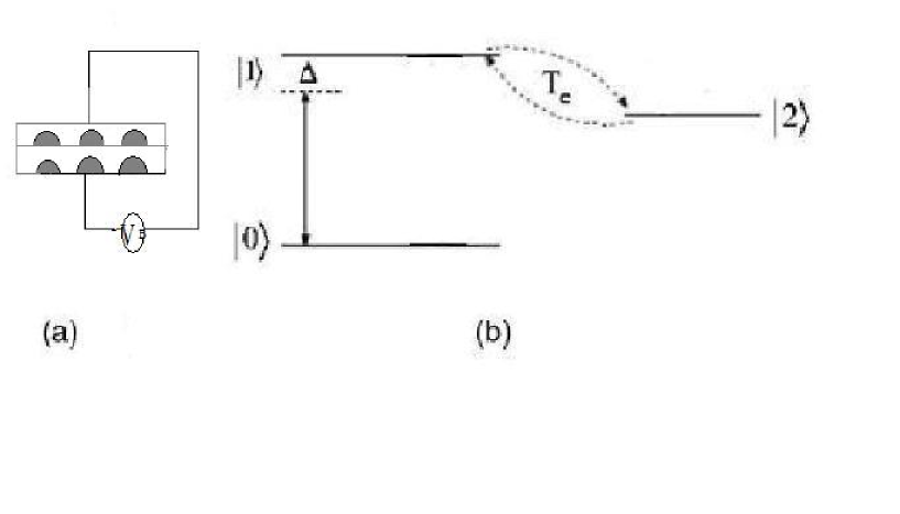
Figure 1: (a)Schematic of the setup. An optical pulse transmits the left QD. $V_{B}$ is a bias voltage. (b)Schematic band structure and level configuration of a double QD system for the electromagnetically induced transparency (EIT) operation. A pulse laser excites one electron from the valence band that can tunnel to other dot,and $|0\rangle$ is the system without excitations, $|1\rangle$ a pair os electron and hole bound in the first dot, and $|2\rangle$ one hole in the first dot with an electron in he second dot.

A vertically coupled InGaAs/GaAs asymmetrical quantum dot molecule consists of two layers of dots (the upper one and the lower one) with different band structures coupled by tunnelling is shown in Fig.1(a). Samples are arrays of GaInAs dots in a matrix of GaAs which are vertically stacked, vertically aligned, and electrically coupled in the growth direction. Dots in two different layers show a strong tendency to align vertically. The coupling is mainly determined by the separation distance of two layers. In this quantum dot system, the lower QD is slightly small, which the energy separation is bigger than the upper one. From the Ref. Krenner , we know that for QD separation $d>9$ nm the tunnelling coupling between the two dots is weak and the QD system can be discussed in terms of a simplified single-particle pictureChun ; Bester . One can excite one electron from the valence to the conduction band in the lower dot which can in turn tunnel to the upper dot by applying electromagnetical field. Figure 1 (a) gives a schematic of the system. The tunnel barrier in an asymmetric quantum dot molecule can be controlled by applying a bias voltage between the $n^{+}$-contact and the Schottky gate. Figure 1(b) depicts an energy-level diagram of an asymmetric quantum dot molecule. The ground state $|0\rangle$ is the system without excitations, and the direct exciton state $|1\rangle$ is a pair of electron and hole bound in the lower dot, and the indirect exciton state $|2\rangle$ is one hole in the lower dot with an electron in the upper dot. Using this configuration the Hamiltonian of the system reads as follows($\hbar=1$)Villas

$$\begin{split}H_{1}=&\sum_{j=0}^{2}\varepsilon_{j}|j\rangle\langle j|+\omega_{c}a_{c}^{+}a_{c}+g_{c}(|1\rangle\langle 0|a_{c}+|0\rangle\langle 1|a_{c}^{+})\\ &+T_{c}(|1\rangle\langle 2|+|2\rangle\langle 1|),\end{split}$$ (1)

where $\varepsilon_{j}$ is the energy of state $|j\rangle$, $T_{c}$ is the electron tunnelling matrix element between two dots, $a^{+}_{c}$ and $a_{c}$ are, respectively, the creation and annihilation operators of the quantized field with frequency $\omega_{c}$. $g_{c}$ is the coupling constant of the quantized field and the direct exciton (the state of $|0\rangle$ and $|1\rangle$). The Hamiltonian $H_{1}$ is rather simple, but it is not complete. Since the double quantum dots is embedded in the macroscopic crystal, the single electron is unavoidably scattered by phonons while tunnelling between two dots. Considering the coupling between electron and phonons, the Hamiltonian can be written as

$$H=H_{1}+\sum_{k}\omega_{k}b_{k}^{+}b_{k}+\\ \frac{1}{2}(|1\rangle\langle 1|-|2\rangle\langle 2|)\sum_{k}g_{k}(b_{k}^{+}+b_{k}),$$ (2)

where $b_{k}^{+}$ $(b_{k})$ and $\omega_{k}$ are the creation (annihilation) operator and energy for $k$th phonon mode, respectively, $g_{k}$ is the coupling constant determined by the crystal material and the geometry of the coupling quantum dots. The electron-phonon interaction in Hamiltonian (2) contains only the diagonal elements, because the role of off-diagonal ones is suppressed at low temperatures. Applying a canonical transformation with the generatorZhuo ; Du

$$S=(|1\rangle\langle 1|-|2\rangle\langle 2|)\sum_{k}\frac{g_{k}}{2\omega_{k}}(b_{k}^{+}-b_{k}).$$ (3)

The transformed Hamiltonian is given by

$$H^{\prime}=e^{s}He^{-s}=H_{0}^{\prime}+H_{I}^{\prime},$$ (4)

where

$$\begin{split}H_{0}^{\prime}=&\varepsilon_{0}|0\rangle\langle 0|+(\varepsilon_{1}-\Delta)|1\rangle\langle 1|+(\varepsilon_{2}-\Delta)|2\rangle\langle 2|\\ &+\sum_{k}\omega_{k}b_{k}^{+}b_{k}+\omega_{c}a_{c}^{+}a_{c}\end{split}$$ (5)

$$H_{I}^{\prime}=g_{c}(|1\rangle\langle 0|X^{+}a_{c}+|0\rangle\langle 1|Xa_{c}^{+})+T_{c}(|2\rangle\langle 1|X^{2}+|1\rangle\langle 2|X^{2+})$$ (6)

$$\Delta=\sum_{k}\frac{g_{k}^{2}}{4\omega_{k}},X=exp[-\sum_{k}\frac{g_{k}}{2\omega_{k}}(b_{k}^{+}-b_{k})].$$ (7)

Here we assume that the relaxing time of the environment (phonon fields) is so short that the excitons do not have time to exchange the energy and information with the environment before the environment returns to its equilibrium state. The excitons interact weakly with the environment so that the equilibrium thermal properties of the environment are preserved. Therefore it is reasonable to replace the operator $X$ with its expectation value over the phonons number states which are determined by a thermal average and write the Hamiltonian asMahan ; Chen ; Zhu1

$$\begin{split}H^{\prime}=&\varepsilon 0|0\rangle\langle 0|+(\varepsilon 1-\Delta)|1\rangle\langle 1|+(\varepsilon_{2}-\Delta)|2\rangle\langle 2|\\ &+\sum_{k}\omega_{k}b_{k}^{+}b_{k}+\omega_{c}a_{c}^{+}a_{c}\\ &+g_{c}e^{-\lambda(N_{ph}+1/2)}(|1\rangle\langle 0|a_{c}+|0\rangle\langle 1|a_{c}^{+})\\ &+T_{c}e^{-2\lambda(N_{ph}+1/2)}(|2\rangle\langle 1|+|1\rangle\langle 2|)\end{split}$$ (8)

where $\lambda=\sum_{k}(g_{k}/2\omega_{k})^{2}$ is the Huang-Rhys factor. Here for the sake of simplicity we only perform the analysis for the simplest case in which only the longitudinal-optical (LO) phonon is considered,i.e., all the phonons have the same frequency Yuan ; Chen ; Zhu1 . We anticipate that this is sufficient to illustrate the main physics in the more complicated case of the acoustic phononsDu . In such a case $\omega_{k}=\omega_{0}$ is irrelevant to the wavevector $k$ of phonon, and the phonon populations can be written as $N_{ph}=\frac{1}{e\frac{\omega_{0}}{k_{B}T}-1}$Mahan ; Chen where $k_{B}$ is Boltzmann constant and $T$ is temperature of the environment. After using the operator $\Lambda=e^{i\sum_{k}\omega_{0}b_{k}^{+}b_{k}}$ to transform to a frame rotating at the frequency $\omega_{0}$, we can cancel the term $\sum_{k}\omega_{0}b_{k}^{+}b_{k}$ in Eq.(8) and get its eigenstates (l=1,2,3)

$$|\psi\rangle^{l}=C_{0}^{l}|0,n+1\rangle+C_{1}^{l}|1,n\rangle+C_{2}^{l}|2,n\rangle,$$ (9)

where $n$ is the photon number of the quantized field,

$C_{0}^{l}=\frac{1}{\sqrt{1+a_{l}^{2}+b_{l}^{2}}}$, $C_{1}^{l}=\frac{a_{l}}{\sqrt{1+a_{l}^{2}+b_{l}^{2}}}$, and $C_{2}^{l}=\frac{b_{l}}{\sqrt{1+a_{l}^{2}+b_{l}^{2}}}$. Here

$$a_{l}=\frac{\eta_{l}-e_{1}}{e_{4}},$$ (10)

$$b_{l}=\frac{e_{5}}{e_{4}}\frac{\eta_{l}-e_{1}}{\eta_{l}-e_{3}},$$ (11)

with $e_{1}=\varepsilon_{0}+(n+1)\omega_{c}$,$e_{2}=\varepsilon_{1}-\Delta+n\omega_{c}$, $e_{3}=\varepsilon_{2}-\Delta+n\omega_{c}$,$e_{4}=g_{c}e^{-\lambda(N_{ph}+1/2)}\sqrt{n+1}$, $e_{5}=T_{c}e^{-2\lambda(N_{ph}+1/2)}$. Also $\eta 1$,$\eta 2$ and $\eta 3$ are the roots of the equation

$$\begin{split}&\eta^{3}-(e_{1}+e_{2}+e_{3})\eta^{2}+(e_{1}e_{2}+e_{1}e_{3}+e_{2}e_{3}-e_{4}^{2}-e_{5}^{2})\eta\\ &+(e_{1}e_{5}^{2}+e_{4}^{2}e_{3}-e_{1}e_{3}e_{3})=0.\end{split}$$ (12)

According to Ref.Fuentes ,the phase shift operator $U(\varphi)=e^{-\varphi a^{+}a}$ is introduced. Applied adiabatically to the Hamiltonian Eq.(8), the phase shift operator alters the sates of the field and gives rise to the following eigenstates:

$$|\psi\rangle_{p}^{l}=C_{0}^{l}e^{-i(n+1)\varphi}|0,n+1\rangle+C_{1}^{l}e^{-in\varphi}|1,n\rangle+C_{2}^{l}e^{-in\varphi}|2,n\rangle$$ (13)

Changing $\varphi$ slowly from 0 to 2$\pi$ , the Berry phase is calculated as $\gamma_{l}=i\int_{0}^{2\pi}{{}_{p}}{{}^{l}}\langle\psi|\frac{\partial}{\partial\varphi}|\psi\rangle_{p}^{l}d\varphi,$ it gives $\gamma_{l}=2\pi[n+(C_{0}^{l})^{2}]$.

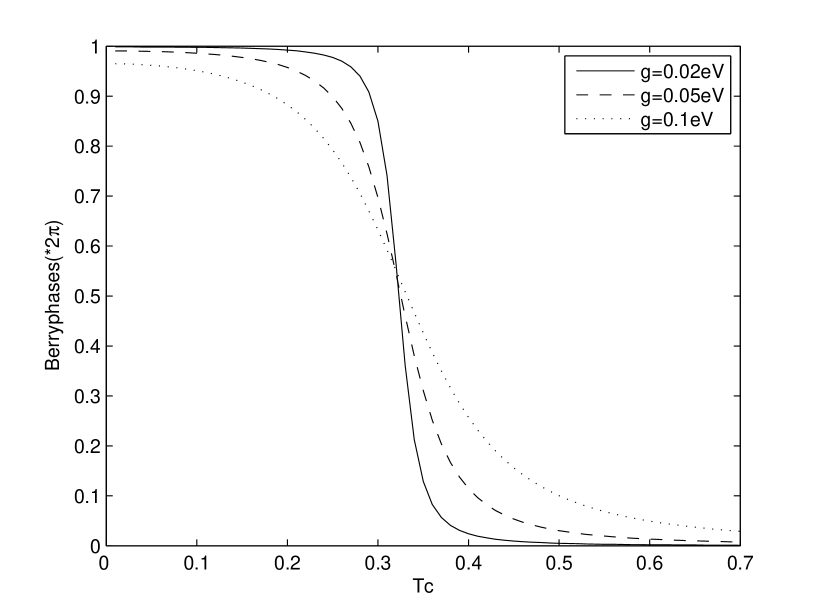
Figure 2: The Berry phases of the system as the function of $T_{c}$ with different $\gamma$,($\gamma_{1}$ solid curve,$\gamma_{2}$ dashed curve)Where $n=0$, $\varepsilon_{0}=0eV$, $\varepsilon_{1}=1.3eV$, $\varepsilon_{2}=1.0eV$, $g=0.02eV$, $\Delta=0.1eV$ $\omegaup_{c}=0.3eV$, $\lambda=0.02eV$, $T=0$

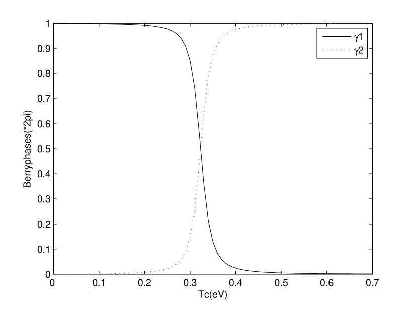
Figure 3: The Berry phases the function of $T_{c}$ with different $g_{c}$, Where $n=0$, $\varepsilon_{0}=0eV$, $\varepsilon_{1}=1.3eV$, $\varepsilon_{2}=1.0eV$, $\Delta=0.1eV$ $\omegaup_{c}=0.3eV$, $\Delta=0.02eV,$T=0

In calculation, $\varepsilon_{0}=0meV$,$\varepsilon_{1}=1.3meV$ and $\varepsilon_{2}=1.0meV$ are be usedLegramd; Findeis; Grandidier. Figure1 shows the variation Berry phases when the tunneling is varied via gate voltage. It is obvious that the Berry phase is different from zero even for the driving field in the vacuum state ($n=0$). As the parameters g chosen, the Berry phase is an approximately 2m$\pi$(m is an integer)shift as the tunneling $T_{c}<0.3eV$ or $T_{c}>0.4eV$. As the result of quantizing the driving field, the term $2m\pi$ is appears in the Berry phase. The range of $T_{c}$ where the Berry phase changes obviously from $2m\pi$ to $2(m\pm 1)\pi$ is related to different coupling constants g. As the coupling constants increase, the changing of the Berry phase are inclining to become slow. From the picture we can see that the Berry phase is changing more sharp when g is 0.01eV than g is 0.1eV. Figure2 show two kinds of Berry phases. There are three Berry phases in all, here we just give two typical kinks of them($\gamma_{1},\gamma_{2}$). The $\gamma_{3}$ does not give a new results. Figure 2 shows the two curves about $\gamma_{1}$ and $\gamma_{2}$ are symmetric.

For the illustration of the numerical results, we choose the vertically coupled InGaAs/GaAs quantum dots as an example for experiments. For such a double dot, we assume that $\varepsilon_{0}=0eV$,$\varepsilon_{1}=1.3eV$ and $\varepsilon_{2}=1.0eV$Krenner1 , $\Delta=0.01eV$ and $\lambda=0.02$Kamada . The LO-phonon energy ($\omega_{0}$) of GaAs is 36 meVMahan . We apply a quantized field with frequency $\omega_{c}=0.3eV$ which is just resonant with the bonding state of the level $|1\rangle$ and the level $|2\rangle$ via the tunnel coupling as shown in Fig.1(a). Figure 2 shows the Berry phases as a function of tunnelling ($T_{c}$) via a bias voltage for three coupling constants ($g_{c}$) at $T=50mK$. It is obvious that the Berry phase is different from zero even for the driving field in the vacuum state ($n=0$), which is in agreement with the results obtained by Fuentes-Guridi et al.Fuentes . By simply tuning by the bias voltage, the Berry phases can be changed dramatically from 2$\pi$ to 0 as the parameter $g_{c}$ is fixed. From Fig.1 we can see that the Berry phase is an approximately 2$\pi$ for the tunnelling $T_{c}<0.8eV$, but as the tunnelling continuously increases to $T_{c}>0.9eV$ the Berry phase is suddenly down to zero. As realized in experiments, we can fix the incident light through a single mode fiber and continuously tuning the bias voltage, if the Berry phase is suddenly changed, then we can detect this predicted effect in an interference experiment. The range of $T_{c}$ where the Berry phase changes obviously from $2m\pi$ to $2(m\pm 1)\pi$ ($m$ is an integer) is related to the different coupling constants ($g_{c}$). As the coupling constants increase, the change of the Berry phase becomes slow. From the figure it is evident that the Berry phases are altered more sharply as $g_{c}=0.02eV$ than $g_{c}=0.1eV$. Figure 3 shows two kinds of Berry phases ($\gamma_{1},\gamma_{2}$) as a function of tunnelling $T_{c}$. In general, there are three Berry phases in all, here we just give two typical kinds of them ($\gamma_{1},\gamma_{2}$). The $\gamma_{3}$ does not give a new result. Figure 3 shows the two curves about $\gamma_{1}$ and $\gamma_{2}$ are symmetrical at $T_{c}\approx 0.85eV$. It should be noted here that the present scheme can also applied to the double quantum dot system realized by Gustavsson et al.Gus , which the driving field is operated at microwave frequency. In such a case, the tunnelling $T_{c}$ can be reached to $meV$ or even to $\mu eV$ through varying the gate voltage.

In conclusion, we have theoretically investigated the voltage-controlled Berry phases in an asymmetry semiconductor double quantum dots. It is found that Berry phases can be changed suddenly from 0 to 2$\pi$ (or 2$\pi$ to 0) only simply by tuning the external voltage. Under realistic experimental conditions, as the tunnelling is varied from $0.8eV$ to $0.9eV$ via a bias voltage, the Berry phase can be altered dramatically. The range of $T_{c}$ where the Berry phase changes obviously from $2m\pi$ to $2(m\pm 1)\pi$ is related to different coupling constant ($g_{c}$). As the coupling constant $g_{c}$ enhances, the change of the Berry phases become slow. This scheme opens up the electrical controllability of the Berry phases which is expected to be useful in constructing quantum computer based on geometric phases in an asymmetric double quantum dot controlled by voltage.

This work has been supported in part by National Natural Science Foundation of China (No.10774101) and the National Ministry of Education Program for Training Ph.D.

References

References

- (1) M.A.Nilsen and I.L.Chuang, Quantum Computation and Quantum Information (Cambridge University Press, Cambridge, UK, 2000).
- (2) A.Shapere and F.Wilczek, Geometric Phases in Physics, (World Scientific, Singapore, 1989)
- (3) J.Anandan, Nature (London)360, 307(1992).
- (4) M.V.Berry, Proc.R.Soc.London Ser. A 392, 45(1984).
- (5) J.A.Jones,V.Vedral,A.Ekert,and G.Castagnoli Nature(London)403,869(1999).
- (6) G.Falci, R.Fazio, G.M.Palma, J.Siewert, and V.Vedral, Nature (London) 407, 355(2000)
- (7) I.Fuentes-Guridi, A.Carollo, S.Bose and V.Vedral, Phys.Rev.Lett.89, 220404(2002).
- (8) X.X.Yi, L.C.Wang, and T.Y.Zheng, Phys. Rev. Lett.92,150406(2004).
- (9) P.San-Jose, B.Scharfenberger, G.Shon, A.Shnirman, and G.Zarand, arXiv:cond-mat/0710.3931(2007).
- (10) X.Z.Yuan and K.D.Zhu, Phys.Rev.B74, 073309(2006).
- (11) Y. Zhang, Y.W. Tan, H. L.Stormer and P.Kim, Nature (London)438,201(2005).
- (12) M. Möttönen,J.J.Vartiainen, and J.P.Pekola, arXiv: cond-mat/0710.5623(2007).
- (13) P.J.Leek, J.M.Fink, A.Blais, Science318,1889(2007).
- (14) H. J. Krenner, M. Sabathil, E. C. Clark, A. Kress, D. Schuh, M. Bichler, G. Abstreiter, and J. J. Finley, Phys. Rev. Lett. 94, 057402 (2005).
- (15) C.H.Yuan and K.D.Zhu, Appl. Phys. Lett.89, 052115(2006).
- (16) G. Bester, A. Zunger and J. Shumway, Phys. Rev. B 71, 075325 (2005).
- (17) J. M. Villas-Bôas, A. O. Govorov, and S. E. Ulloa, Phys. Rev. B 69, 125342 (2004).
- (18) Z.J.Wu, K.D.Zhu, X.Z.Yuan, Y.W.Jiang and M.Yao, Phys. Lett. A 347, 251(2005)
- (19) C.R.Du and K.D.Zhu, Phys. Lett. A372, 537(2007).
- (20) G.D.Mahan, Many-Particle Physics (Plenum, New York,1981)
- (21) Z.Z.Chen, R.Lu, and B.F.Zhu, Phys.Rev.B 71, 165324(2005).
- (22) C.H.Yuan, K.D.Zhu, X.Z.Yuan, Phys. Rev.A 75, 62309(2007).
- (23) H.J.Krenner,S.Stufler, M.Sabathil, E.C.Clark, P.Ester, M.Bichler, G.Abstreiter, J.J.Finley and A.Zrenner, New J.Phys. 7, 184(2005).
- (24) H.Kamada, H.Gotoh, J.Temmyo, T.Tagagahara, H.Ando, Phys. Rev. Lett. 87, 246401(2001).
- (25) S.Gustavsson, M.Studer, R.Leturcq, T.Ihn,K.Ensslin, D.C.Driscoll and A.C.Gossard, Phys. Rev. Lett. 99,06804(2008).