Average Properties of a Large Sample of $z_{abs}\sim z_{em}$ associated Mg II Absorption Line Systems

Abstract

We have studied a sample of 415 associated ($z_{abs}\sim z_{em}$; relative velocity with respect to QSO $<$ 3000 ${\rm km\;s}^{-1}$) Mg II absorption systems with 1.0$\leq z_{abs}\leq$1.86, in the spectra of Sloan Digital Sky Survey, Data Release 3 QSOs, to determine the dust content, ionization state, and relative abundances in the absorbers. We studied the dependence of these properties on the properties of the backlighting QSOs and also, compared the properties with those of a similarly selected sample of 809 intervening systems (apparent relative velocity with respect to the QSO of $>$ 3000 ${\rm km\;s}^{-1}$), so as to understand their origin. Normalized, composite spectra were derived, for absorption line measurements, for the full sample and for several sub-samples, chosen on the basis of the line strengths and other absorber and QSO properties. Composite absorption lines differ in small but measurable ways from those in the composite spectra of intervening absorption line systems, especially in the relative strengths of Si IV, C IV and Mg II. From the analysis of the composite spectra, as well as from the comparison of measured equivalent widths in individual spectra, we conclude that the associated Mg II absorbers have higher apparent ionization, measured by the strength of the C IV absorption lines compared to the Mg II absorption lines, than the intervening absorbers. The ionization so measured appears to be related to apparent ejection velocity, being lower as the apparent ejection velocity is more and more positive. Average extinction curves were obtained for the sub-samples by comparing their geometric mean QSO spectra with those of matching (in $z_{em}$ and $i\;{\rm magnitude}$) samples of QSOs without absorption lines in their spectra. There is clear evidence for dust-like attenuation in these systems, though the 2175 Å absorption feature is not present: the extinction is similar to that found in the Small Magellanic Cloud. The extinction is almost twice that observed in the similarly selected sample of intervening systems. We reconfirm with our technique that QSOs with non-zero FIRST (Faint Images of the Radio Sky at Twenty-cm) radio flux are intrinsically redder than the QSOs with no detection in the FIRST survey. The incidence of associated Mg II systems in QSOs with non-zero FIRST radio flux is 1.7 times that in the QSOs with no detection in the FIRST survey. The associated absorbers in radio-detected QSOs which comprise about 12% of our sample, cause three times more reddening than the associated absorbers in radio-undetected QSOs. The origin of this excess reddening in the absorbers is indicated by the correlation of the reddening with the strength of Mg II absorption. This excess reddening possibly suggests an intrinsic nature for the associated absorbers in radio-detected QSOs.

1 Introduction

Many of the first detected, narrow-line QSO absorption systems had redshifts close to those of their QSOs (e.g. Stockton & Lynds 1966; Burbidge, Lynds & Burbidge 1966). Such systems, having a relative velocity with respect to the QSO, in units of the speed of light, $\beta$, smaller than 0.02, are now termed associated systems. Study of the associated systems is important from the point of view of understanding the energetics and kinematics near the central black hole and also for understanding the ionization structure, dust content and abundances in material directly exposed to the radiation from the QSOs, and in some cases, possibly ejected from, the QSOs or the accretion disks. Associated systems have been suggested to arise (a) in the outer parts of QSO host galaxies (e.g. Heckman et al. 1991; Chelouche et al. 2007) which may have gas properties similar to those in the outer parts of inactive galaxies (Steidel et al. 1997, Fukugita & Peebles 2006); (b) by material within 30 kpc of the AGN, accelerated by starburst shocks from the inner galaxy (e.g. Heckman et al. 1990, 1996; D’Odorico et al. 2004; Fu and Stockton 2007a); (c) in the core of the AGN, within 10 pc of the black hole (Hamann et al. 1997a; Hamann et al. 1997b; Barlow & Sargent 1997).

In case (a), these are possibly “halo” clouds as in normal galaxies, possibly lit up by the QSO to produce extended regions of Lyman alpha emission, but not thought to be moving at the high velocities necessary to explain the dispersion of associated system velocities with respect to the QSO itself. However, using spectra of a set of angularly close QSO pairs, Bowen et al. (2006) confirmed that gas in the outer parts of some QSO host galaxies is detectable as absorption in the spectra of background QSOs, but the spectra of the foreground QSOs did not reveal associated absorption systems: evidently, the appearance of the absorption is dependent on the angle of the line of sight to the spin axis of the accretion disk. The low velocities expected from such gas led to the postulate that clusters of galaxies near the QSO showing associated absorption were responsible for the absorption and the dispersion of cloud velocities. However, QSOs are not only associated with clusters of galaxies: they appear in a wide range of galaxy types and masses (Jahnke et al. 2004) and, while found in slightly higher density environments (Serber et al. 2006), do not require cluster type densities on large scales (Wake et al. 2004).

In case (b), the gas is typically found to have densities of a few hundred particles cm^-3, high enough to produce excited fine structure lines of Si II and C II. There are suggestions in the above references that this is material ejected by a galactic wind, possibly a superwind from a starburst (Heckman et al. 1990), then lit up by the QSO. (These are often called extended emission line regions, EELR). Cooling flows (Crawford & Fabian 1989) no longer seem to be considered in most cases (Fu & Stockton 2007b).

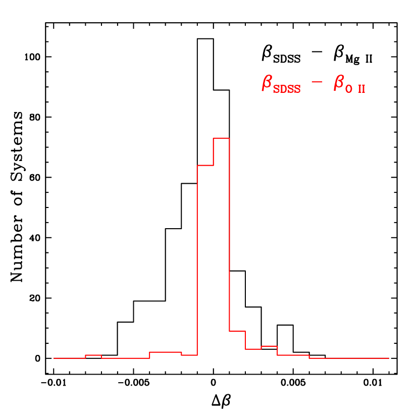
Figure 1: The difference between the $\beta$ values derived for the Mg II associated absorption systems using SDSS redshifts ($\beta$_SDSS)and (red) the single line [O II] ($\beta$${}_{\rm O\;II}$) or (black) the single line Mg II redshifts ($\beta$${}_{\rm Mg\;II}$). [O II] is available for 162 QSOs, Mg II is available for 415 QSOs. The single line [O II] and Mg II emission line redshifts are derived from the SDSS pipeline. The [O II] line is regarded as giving the best systemic redshift when it is available. The $\beta$ [O II] values agree very well with the derived SDSS values, which are used in this paper.

In case (c), absorption is inferred to be very close to the black hole because of variability in the absorption lines, and/or because of the presence of clouds that do not cover the source. Theoretical investigations of case (c) (Arav et al. 1994; Konigl & Kartje 1994; Murray et al. 1995; Krolik & Kriss 2001; Proga et al. 2000; Everett 2005; Chelouche & Netzger 2005 (for a Seyfert galaxy with a much lower radiation field)), have reinforced the plausibility of thermal or hydromagnetic, radiation assisted flows, both parallel to the AGN jet axis, and perpendicular to it, along the accretion disk. See, for example, Figure 13 of Konigl & Kartje (1994), Figure 1 of Richards et al. (1999), Figure 1 of Murray et al. (1995) and Figure 1 of Everett (2005).

Early studies concentrated on systems with C IV doublets. Weymann et al. (1979) and Foltz et al. (1986) found a statistical excess of such systems as compared to what was expected if these were randomly distributed in space. Other studies (Young et al. 1982; Sargent et al. 1988) could not confirm these observations. Later it was shown that Mg II systems (Aldcroft et al. 1994) and C IV systems (Anderson et al. 1987; Foltz et al. 1988) with $\beta$$<$ 0.0167 are preferentially found in steep-spectrum radio sources, often thought of as sources dominated by emission from lobes rather than the core of the source. Ganguly et al. (2001) showed that high ionization systems (having lines of C IV, N V and O VI) with $\beta$$<$ 0.0167 with $z_{abs}<1.0$ are not present in radio-loud QSOs that have compact radio morphologies, flat radio spectra (core dominated sources) and C IV lines with mediocre FWHM ($\leq 6000$ ${\rm km\;s}^{-1}$). Baker et al. (2002) from a study of a near-complete sample of low-frequency selected, radio-loud QSOs corroborated trends for C IV associated absorption to be found preferentially in steep-spectrum and lobe-dominated QSOs, suggesting that the absorption is the result of post-starburst activity and that the C IV lines weaken as the radio source grows, clearing out the gas and dust. Vestergaard (2003, hereafter V03) studied a sample of high ionization associated systems with $1.5<z_{abs}<3.5$ and found that the occurrence, or not, of such systems is independent of radio properties of the QSOs. V03 did not find the relationship between radio source size and C IV line strength of Baker et al. (2002), nor the absence of absorbers in low line width systems of Ganguly et al (2001). V03 did identify weak correlations among QSO properties and the line strengths of the associated absorption systems, that differed from those of the intervening systems, but concluded that differences in the results among the three studies (Baker et al. 2002; Vestergaard 2003 and Ganguly et al. 2001) could probably be attributed to various differences in selection of the relatively small samples ( 50-100 systems): among them, the most obvious difference is the optical luminosity of the samples, progressively more luminous in order of the references just cited.

Steep spectrum radio sources, from the above references, have an excess of associated ($\beta$$<0.02$) absorbers and are thought to be viewed at a large angle to the jet axis, so the sightline passes over the accretion disk (or torus). Broad absorption line (BAL) systems are often thought to be viewed from the same aspect, but are generally devoid of radio flux. There are suggestions that the associated systems are related in some way to the broad absorption line systems (Wampler et al. 1995; Baker et al. 2002; V03), summarized by V03.

There have also been suggestions that narrow line QSO absorption line systems (QSOALS) that have high velocities with respect to the QSO, i.e. apparent velocities of ejection up to tens of thousands of ${\rm km\;s}^{-1}$ may also be associated with the QSOs i.e. they are close to the QSO ($<<$ 10 pc) but have high relative velocity (Vanden Berk et al. 1996; Januzzi et al. 1996; Richards et al. 1999; Richards 2001; V03; Misawa et al. 2007); candidate systems are especially noticeable in the brightest QSOs and in radio sources with flat radio spectra (often said to be core-dominated sources). Richards et al. (2001), using the largest sample of radio QSOs available to date, showed that there is an excess of C IV absorbers at high $\beta$ values in flat spectrum radio sources (thought to be viewed close to the jet axis), strengthening arguments of Richards et al. (1999) and Richards (2001) that up to 36% of the apparently high velocity material is associated with material intrinsic to the background AGN. As shown by Misawa et al. (2007), such material may evidently reach very high outflow velocities, up to and exceeding 20,000 ${\rm km\;s}^{-1}$. Their evidence for the intrinsic nature of such components is the small filling factor of the absorption lines in covering the background UV radiation source, presumably the full accretion disk (Pereya et al. 2006). A primary question is how to tell if a given system is intrinsic or not, whatever its $\beta$ value.

In this paper, we use a large and homogeneous sample of associated ($z_{abs}\sim z_{em}$; relative velocity with respect to the QSO $<$ 3000 ${\rm km\;s}^{-1}$) Mg II systems with $1.0<z_{abs}<1.86$ compiled from the Sloan Digital Sky Survey (SDSS) Data Release 3 (DR3) catalog to determine the average dust content, ionization and relative abundances in these absorbers. Our aim is to determine if these systems are indeed intrinsic to the QSOs by (a) studying the dependence of their average properties on QSO properties and (b) comparing the properties of associated, Mg II systems with those of intervening systems ($\beta$$>$ 0.01) selected with similar criteria. In particular, we are looking for a spectroscopic signature to distinguish associated from intervening systems.

We make use of the composite spectra of the sample (and various sub-samples thereof), following the method recently advocated by York et al. (2006, hereafter Y06). In Section 2, we describe the criteria used for sample selection, various sub-samples generated from the main sample and the method of generating composite spectra. In section 3, we present our results which include (i) a comparison between the properties of the samples of the intervening and associated systems, using several statistical tests; (ii) a discussion of the line strengths in the composite spectra of associated systems compared to those for the intervening sample and of the state of ionization in these systems; (iii) the measured extinction for various sub-samples; (iv) a detailed analysis of the dependence of extinction and other properties on the radio properties of the QSOs; (v) discussion of the abundances in associated sample; and (vi) possible scenarios for the origin and location of the absorbers. A few systematic effects that may be hidden in our data are noted in section 4. Conclusions are presented in section 5.

2 Analysis

2.1 Sample selection

The absorption line system sample used here was selected from the SDSS DR3 absorption line catalog compiled by York et al. (2005, 2006). In this section we describe the SDSS, the QSO sample in which the absorbers are discovered, the construction of the SDSS absorber catalog, and finally the selection of the associated absorption line systems used in this study.

The SDSS (York et al. 2000, Stoughton et al. 2002) is an imaging and spectroscopic survey carried out from Apache Point Observatory, near Sunspot, New Mexico, using a 2.5 meter telescope (Gunn et al. 2006). Candidate QSOs are color-selected from 5 color scans with a CCD camera (Gunn et al. 1998) of the 10,000 square degrees of the sky north of Galactic latitude 30 degrees. The photometry from that imaging survey is based on a specially constructed set of filters (Fukugita et al. 1996), calibrated with tertiary standards in the imaging scans (Tucker et al. 2006). The establishment of secondary standards using the SDSS Photometric Telescope (Hogg et al. 2001) and the 1-meter telescope at the US Naval Observatory (Flagstaff), and their tie to a primary standard, is described by Ivezic et al. (2004) and Smith et al. (2002). The photometry is better than $\pm$ 0.02 magnitudes in all bands (Adelman-McCarthy et al. 2007)

The QSOs are color selected (Richards et al. 2002a) from the reduced, archived photometric data. Spectra are obtained using two, dual spectrographs. Plates are drilled with 640, 3 arcsec diameter holes, distributed over an area of seven square degrees, into which optical fibers are inserted by hand. About 100 of the fibers are allocated to QSOs. The selection of QSOs is meant to be complete to magnitude 19.1 in the SDSS $i$ band, except that two objects within 55 arcsec of each other can not be observed using the same plate: one QSO must sometimes be picked over another, or a galaxy may take higher priority over a nearby QSO in the plate planning process. (Multiple, adjacent QSOs exist in the archive because a second plate can be planned to overlap with a previous plate (Blanton et al. 2003)). The astrometry, accurate to $<$ 0.1 arcsec, that allows precise placement of the fibers is described by Pier et al. (2003). The plates are manually plugged and are used on nights not normally acceptable for imaging. Typically forty-five to sixty minutes of exposure are obtained in several, 15-minute integrations, when cloudless skies prevail. The exposure times or the total number of exposures are adjusted so the end result yields (S/N)${}^{2}\sim$7 for an object of $g$ magnitude 20.1. The selection of objects yields a set of QSO spectra with about 70% efficiency (some selected objects are not QSOs), complete to better than 90% (Vanden Berk et al. 2005). Each plate includes fibers allocated to standard stars for flux calibration and for sky removal. Below $i$=19.1, QSOs are also, included in the selection if they are X-ray sources from ROSAT (Voges et al. 1999) or radio sources from the VLA FIRST (Faint Images of the Radio Sky at Twenty-cm) survey (Becker et al. 1995).

These spectra are reduced with two pipelines (two dimensional extraction and one dimensional analysis). The QSO emission redshift is determined, by the SDSS pipeline, by first assembling a list of emission peaks using a wavelet based, peak-finding algorithm. These are matched against a standard set of strong QSO emission lines to find the best-fit redshift (SubbaRao et al. 2002).

The assembly of the archive of all QSOALSs in the spectra occurs in a separate pipeline (York et al. 2005), run after the authoritative QSO spectra are prepared for publication (Schneider et al. 2005 for DR3, Schneider et al. 2007 for DR5). A more complete description of the pipeline is in preparation (York et al., in preparation). Briefly, significant (equivalent width $>$ 3 $\sigma$, $\sigma$ being the uncertainty in the equivalent width measurement due to noise in the spectrum; for narrow line QSOALS, the continuum error is smaller, in general, than the error due to noise.), narrow (typically 3-8 pixels, each 70 ${\rm km\;s}^{-1}$ in width) absorption features are identified after fitting a smooth continuum to the spectrum. Poor night sky subtraction is easily recognized and features found do not include such artifacts. BALs are identified and flagged separately (Trump et al. 2006, for DR3, the data release used in this paper): no lines are picked for this study from QSOs that contain known BALs. However, most BALs in the SDSS are detected by the presence of C IV absorption, and only a small fraction have detectable Mg II absorption (e.g. Trump et al. 2006). About half of the QSOs in our sample of associated absorbers (described below) have $z_{em}$$<$ 1.5 and cannot be determined to be free of BAL systems, since C IV emission is not redshifted into the SDSS spectra until $z_{em}$$\geq$ 1.5. A search is first done for C IV doublets (one line is picked and other line with the correct separation in wavelength is searched for), then for Mg II doublets, then for various Fe II pairs of lines (in case one line of Mg II is exactly at one of a select set of night sky lines, or is obliterated by a poor correction for other lines).

Other lines are then selected by their correspondence to the Mg II, Fe II or C IV candidate systems. Unidentified lines are cataloged. These catalogs have been carefully checked by hand to verify that our selection is not missing some extreme situations that are not “normal” but would be extremely interesting if real. Thousands of systems have been examined and the rules above are secure. Among lines identified as being within a line width of the main lines noted above; those that are significant at the 4 $\sigma$ level; those identified as being unambiguous (i.e., not possibly blended with a line from another absorption line system); and those not in the Lyman alpha forest of that QSO, are selected to provide a quality grade for each system. Four such selected lines produces a grade A system; three lines, grade B system; two lines, grade C system. Systems with only one line above a 4 $\sigma$ significance, and those with lines that that are all detected with a significance between 3 and 4 $\sigma$, are, respectively, considered for classification as grade D or E systems. The lines used for grading are primary lines usually seen in QSO absorption line systems: not all detected lines are used, even if they fit all the other requirements. For instance, Fe I is not used, because any time that line would be seen, Fe II would be present and stronger. This set of rules is constantly checked by eye, again, to not avoid recognition of potentially interesting systems. The lines used for grading are the strongest lines of Mg I, C II, Mg II, Al II, Fe II, Al III, C IV and Si IV. Under this set of protocols, for instance, C IV-only systems would be given grades of C, while systems with significant C IV lines accompanied by a line of Si IV or Mg II would be given grades of B, at least. If multiple Si IV and/or Mg II, or gradable lines of other species are present in the systems, the grades would be A.

The catalog thus constructed can be subjected to an SQL search that produces the sample of systems that one is interested in. For this study, we selected grade A systems, containing Mg II lines with the stronger member of the doublet having W${}_{\rm Mg\;II}$ $>0.3$ Å that are not in BAL QSOs; have absorber redshifts 1.0$\leq$ $z_{abs}$$\leq$1.86; have $\beta$$<$ 0.01; and are in QSOs that have $z_{em}$$<$ 1.96. Each system was verified by visual inspection and any BALs present were eliminated. These systems form our main sample (sample # 1) consisting of 415 systems. The list of QSOs in this sample along with their properties ($z_{em}$, $z_{abs}$, $\beta$, $i\;{\rm magnitude}$ and $\Delta(g-i)$) are given in Table 5, in the appendix. The absorber rest-frame equivalent widths of the prominent lines, along with 1 $\sigma$ errors, are given in Table 6 of the appendix. About 100 out of these do have additional grade A and B systems (at absorption redshifts $<<$ $z_{em}$) in their spectra. In principle, these can contribute to the reddening of the parent QSO spectrum, but we show in the next section that they do not contribute to the extinction. Lines in those systems do not contribute to our composite spectrum used for measuring absorption lines because they are masked before averaging the spectra.

The reasons for the particular selection of systems described above are as follows. It is generally believed (e.g. Rao & Turnshek 2000, Churchill et al. 1999) that systems with ${\rm W}_{\rm Mg\;II}$$>$ 0.3 Å have ${\rm N}_{\rm H\;I}$$>3\times 10^{17}$ cm^-2. Thus, the Mg II line strengths were restricted so as to choose systems that might have sufficiently large column densities in H I, so as to have significant dust columns. The redshift range of the absorbers was chosen to allow, on the one hand, only objects for which the 2175 Å feature lies completely within the SDSS spectrograph wavelength range, and, on the other hand, to assure the Mg II lines are at $\lambda<$8000 Å, to avoid the regions of the SDSS spectra that are contaminated by strong night sky emission lines. The restriction on $z_{em}$was imposed to keep the Lyman $\alpha$ forest out of the SDSS spectra. We use the range $\beta<0.01$, to get the purest sample of associated systems possible on the presumption that the higher the $\beta$ the more likely there are intervening systems mixed in. We wish to emphasize that the selection criteria were taken to be same as those used by Y06 (except for the range of $\beta$ values). This was done so that we can compare the properties of the intervening systems (studied by Y06) with those of associated systems (systems with $z_{abs}$$\simeq$ $z_{em}$, studied here) without any selection bias. Such a comparison may indicate some signatures that may point towards the latter systems being intrinsic to the QSOs. Our use of class A systems precludes including C IV-only or Mg II-only systems, and we plan to study those systems in a later paper.

Having made the choice to study Mg II associated systems because we already have a comparison sample of intervening systems, we nevertheless find that our selection is typical, despite the preference of previous authors to focus mainly on systems with C IV and higher ions. First, examination of the complete set of systems selected (Table 5,6) reveals that 89% have significant C IV lines, when those lines are observable in SDSS spectra. Second, a preliminary study of the statistics of all class A and B absorption line systems as a function of $\beta$ (avoiding systems in BAL QSOs) revealed that the peak in the number distribution of C IV systems for -0.003$<\beta<$0.01 is mimicked when Mg II systems are used (without reference to whether they have C IV or not) These statistics will be the subject of a future paper (Vanden Berk et al., in preparation).

A remark is in order about the values of $\beta$ derived. Gaskel (1982) and Wilkes (1984) showed that the redshifts of QSOs differ from line to line. As summarized by Richards et al (2002b), the [O III] redshifts generally agree with the stellar absorption line redshifts of the host galaxies of the QSOs, when these can be observed. The shifts of Mg II emission compared to the rest frame narrow emission line regions defined by [O II] and [O III] is $<$ 200 ${\rm km\;s}^{-1}$(Vanden Berk et al. 2001, Tytler & Fan 1992) and probably about -100 ${\rm km\;s}^{-1}$(Richards et al. 2002b). Richards et al. (2002b) and Richards (2006) studied this effect in SDSS QSOs and advocated the removal of the systematic shift mainly caused by the asymmetric profile of the C IV emission blend by using the wavelength of 1546 Å instead of the normal 1549 Å. This procedure is adopted in the SDSS pipelines. For 250 QSOs in our sample, the C IV line is available and used in deriving the redshift from the SDSS data, by the SDSS pipeline. The species Mg II and [C III] are available for all spectra. The system redshift reference, [O II] is covered in several spectra, but not always detected. Figure 1 shows the comparison of relative velocities of the absorption systems (with respect to the QSOs), namely $\beta$_SDSS, $\beta$${}_{\rm[O~{}II]}$ and $\beta$${}_{\rm Mg~{}II}$, respectively obtained using the (a) SDSS emission redshifts (described above), (b) single line [O II] redshfits when available (for 162 systems in our sample) and (c) single line Mg II redshifts (available for all QSOs in our sample, by selection). The single line [O II] and Mg II redshifts are obtained from the SDSS pipeline. It is apparent that the procedure adopted by the SDSS pipeline does very well in picking the systemic redshifts of the QSOs, and we adopt them in this paper. These redshifts are statistically more precise than the single line redshifts which are sometimes based on weak lines. The errors in $\beta$ are generally $<$ 500 ${\rm km\;s}^{-1}$ where we can check directly with [O II]. We therefore feel the trends we discover later are not caused by errors in the QSO redshifts used here. Letawe et al. (2007), from an analysis of 5 objects, have shown that the peak of H$\beta$ line may be a good indicator of systemic redshifts. However, for our sample ($z_{em}$$>$ 1) the H$\beta$ lines are outside the SDSS spectra, and can not be used to determine the systemic redshifts.

2.2 Generation of arithmetic mean and geometric mean composite spectra

Composite spectra in the absorber rest frame were generated in order to compare continuum and absorption properties of various sub-samples of absorption systems. Both arithmetic mean and geometric mean spectra were generated; the arithmetic mean produces a better representation of the average absorption line profiles, while the geometric mean is better at preserving the continuum properties of the QSOs. The procedure for generating the composites is summarized here, and fully described by Y06.

For the analysis of absorption lines, normalized arithmetic mean spectra were generated as follows. The spectra of individual QSOs were corrected for Galactic reddening (Fitzpatrick 1999; Schlegel et al. 1998) and (along with the associated error arrays) normalized by reconstructions of the QSO continua, using the first 30 QSO eigenspectra derived by Yip et al. (2004). The normalized spectra were shifted to the absorber rest frame and re-sampled onto a common pixel-to-wavelength scale. Pixels flagged by the spectroscopic pipeline as possibly bad in some way (Stoughton et al. 2002) were masked and not used in constructing the composites. Also masked were the pixels within 5 Å of the expected line positions of detected absorption systems unrelated to the target system. The normalized flux density in each remaining pixel was weighted by the inverse of the associated variance, and the weighted arithmetic mean of all contributing spectra was calculated for each pixel. The number of individual spectra, and the distribution of absorber redshifts, contributing to the composite spectrum of a particular line transition, varies from line to line. That is because the absorption system sample was selected to simultaneously cover the Mg II doublet and 2175 Å feature, which means that other transitions may not be covered by all of the spectra. The rest wavelength range of maximum sensitivity to absorption features in the composite spectra, which gets contributions from all QSOs in the sample, is 1900 Å to 3150 Å: the rest frame spectrum of a QSO with absorption system at $z_{abs}$ of 1 will cover the range 1900-4500 Å while that of a QSO with an absorption system at $z_{abs}$ of 1.86 will cover the range 1330-3150 Å. Thus, the C IV lines are averages of spectra of QSOs with absorption systems with $z_{abs}$$>$ 1.4765, while the Ca II lines are averages of spectra of QSOs with absorption systems with $z_{abs}$$<$ 1.267. Accordingly, the apparent noise in the composite spectra near these lines is greater than that near lines which fall in the rest frame 1900-3150 Å region (which gets contributions from all systems of the sample). Therefore, the mean Ca II line and the mean C IV line cannot be assumed to give an average picture of the relative behavior of the two lines. A sub-sample must be confined to appropriate $z_{abs}$ ranges so that all systems averaged include coverage of all the lines to be compared.

For studying the dust content of the absorbers by its effect on the QSO continua, geometric mean QSO spectra in the absorber rest frame were generated. The procedure for generating the geometric mean spectra is similar to that for the arithmetic mean spectra, except that the individual spectra were not normalized, and the arithmetic means of the logarithmic flux densities of the non-masked pixels were calculated (producing geometric means in linear flux density). For each absorber sub-sample composite spectrum, a geometric mean spectrum was generated for a QSO sample matched in SDSS $i$ magnitude and QSO redshift, but without absorption line systems of grades A, B, or C in their spectra. The matching of $z_{em}$ and $i\;{\rm magnitude}$ means that the absolute $i$ magnitudes of the absorber and non-absorber pair also match. The matched, non-absorber spectra were shifted in the procedure to the same rest frames as their absorption sample counterparts, to produce composite non-absorber spectra that can be compared directly to the composite absorber spectra. There are 9737 QSOs in the SDSS DR3 data set available for use in the matched non-absorber samples in the redshift range of interest here; they are free of detected absorption systems, but otherwise satisfy the same selection criteria as QSOs in the absorber sample. The details of the selection of the matching non-absorber sample are described in Y06. The list of QSOs in the set of best matched non-absorbers spectra (for the full absorber sample #1) is given in Table 5 of the appendix.

The ratio of the geometric mean composite spectra of the absorber sample to that of the non-absorber sample is the relative shape of the backlighting QSO continuua, with and without absorption systems. We interpret the ratio as the extinction curve due to dust associated with the absorption systems. It was shown by Y06 that these ratios, produced using various sub-samples of intervening absorption line systems, can be well fit by an SMC extinction law, with different values of the color excess $E(B-V)$. In the same way we fit SMC extinction curves to the geometric mean spectra ratios for our current samples, to derive values of $E(B-V)$ for associated systems. In none of the absorber samples did a Milky Way type extinction curve provide a better fit, and we report only the results for the SMC type fits.

To assess the uncertainty of the relative extinction curves, and the derived values of $E(B-V)$, five independent (without any QSOs in common) matching non-absorber samples were selected for each absorber sample. The first non-absorber sample (given in Table 5 of the appendix) selects the closest matching (in $z_{em}$ and $i\;{\rm magnitude}$) non-absorber QSOs. The subsequent non-absorber samples use the QSOs with next best matches, not already used in the previous non-absorber samples. The largest average differences between the $z_{em}$ and $i\;{\rm magnitude}$ of the absorber and non-absorber QSOs in the 5^th non-absorber sample are $<\Delta z>$=0.03 and $<|\Delta i|>$ =0.07. Composite spectra were constructed and $E(B-V)$ values were obtained for each of the five non-absorber samples for the absorber sample. The five values of $E(B-V)$ were averaged to define the $E(B-V)$ of the absorber sample. The rms dispersion of the five samples (of order $\pm$0.004 magnitudes, attributable to sample selection randomness) was used as a measure of the uncertainty in the values of $E(B-V)$. The derived values of $E(B-V)$ and the associated uncertainties are given in Table 1 for each absorber sub-sample. We conclude that for comparison of extinctions between our sub-samples, differences of 0.01 in $E(B-V)$ are significant and are not caused by systematic errors in defining the continuum. It is possible that a few of the non-absorber QSOs have high intrinsic extinction and the presence of such QSOs in a non-absorber sample will reduce the value of $E(B-V)$. The use of five independent non-absorber samples for determining the $E(B-V)$ values minimizes the effect of such rare non-absorber QSOs. The sub-samples are described next in § 2.3.

2.3 Sub-sample definitions

The full sample (#1) was divided into several sub-samples based on the absorber and QSO properties to study the dependence of the dust content, ionization properties and relative abundances on these properties. The sub-samples were, initially, defined based on dividing the full sample by absolute $i\;{\rm magnitude}$; Mg II equivalent width; $\beta$ (positive or negative); negative $\beta$ (further divided into two); and radio detection/non-detection by the VLA FIRST survey. Specifically, we divided sample 1 into pairs of sub-samples in three different ways: by absolute $i$ magnitude, at the median value of -26.49 (# 2 and 3); by W${}_{\rm Mg\;II}$, at the median value of 1.35 Å (# 4 and 5); and by $\beta$, $<$ 0 or $>$ 0 (# 6 and 7). Sample 6 was further subdivided into 2 sub-samples at the median $\beta$ value of -0.0022 (# 8 and 9).

In order to study the dependence of the properties of the associated absorbers on the radio properties of the QSOs, the full sample was divided into sub-samples based on the detection or non-detection of the QSOs by the FIRST survey (for those QSOs covered by the FIRST survey); these sub-samples are designated #10 (hereafter, RD (radio-detected) QSOs) and #11 (hereafter, RUD (radio-undetected) QSOs). The completeness limit of the FIRST survey catalog across the survey area is 1 mJy (Becker et al. 1995); undetected QSOs have 20 cm fluxes less than this value. Miller et al (1990) define radio loud QSOs to be those having 1.4 GHz luminosities greater than 10²⁵ W/Hz. Thus the RD QSOs with $z_{em}$$<$ 2.0, in the FIRST survey are radio-loud. As all the QSOs in our sample have $z_{em}$$<$ 1.96, our radio-detected and radio-undetected sub-samples can be considered to be sub-samples of radio-loud and radio-quiet QSOs according to the definition of Miller et al (1990).

In order to study the difference in ionization state (measured by the strength of the C IV absorption lines compared to the Mg II absorption lines) of the associated ($\beta$$<$ 0.01) and intervening ($\beta$$>$ 0.01) systems, we constructed a sub-sample (# 12) of associated systems with $z_{abs}$$>1.4675$ so that the wavelength of the C IV lines would be covered by the SDSS spectrum. Sub-sample #12 was sub-divided into two parts (#13 and 14) depending on $\beta$ being $>$ or $<$ 0.

The required sub-samples of intervening systems, for comparison, are as follows. Y06 compiled a sample of 809 intervening systems (hereafter SY06) satisfying the same criteria for selection as used here, except for having $\beta$$>$0.01. This forms our main sample of intervening absorbers. For ionization studies, we selected a sub-sample of SY06 having $z_{abs}$$>1.4675$ (sub-sample SY06CIV). We also defined sub-samples based on radio detection or non-radio detection, from the Y06 intervening sample, for comparison with the associated sample. These two samples are referred to as SY06RD and SY06RUD, respectively.

Properties of various sub-samples (including those of intervening samples) are listed in Table 1 which includes the defining criteria, the average and rms dispersion of $E(B-V)$ values obtained by using the five independent, non-absorber samples, along with the average values of W${}_{\rm Mg\;II}$, $\beta$, $z_{ab}$, $i$ magnitude, absolute $i$ magnitude calculated using the concordance cosmology and $\Delta(g-i)$ .

3 Results

3.1 Comparison of properties of intervening and associated systems

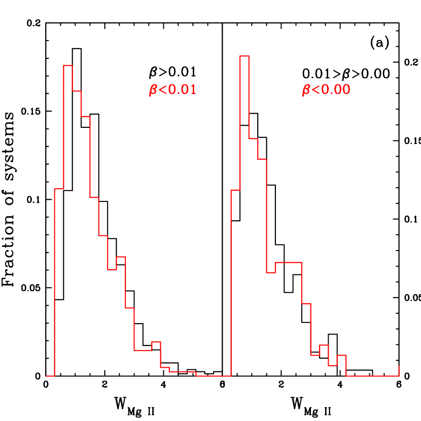
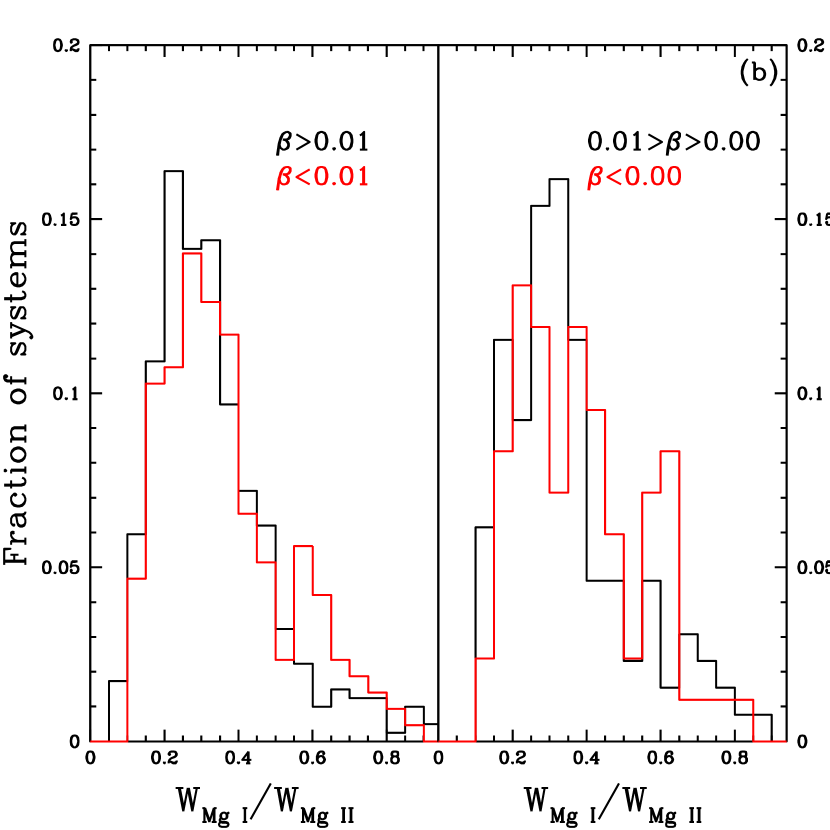
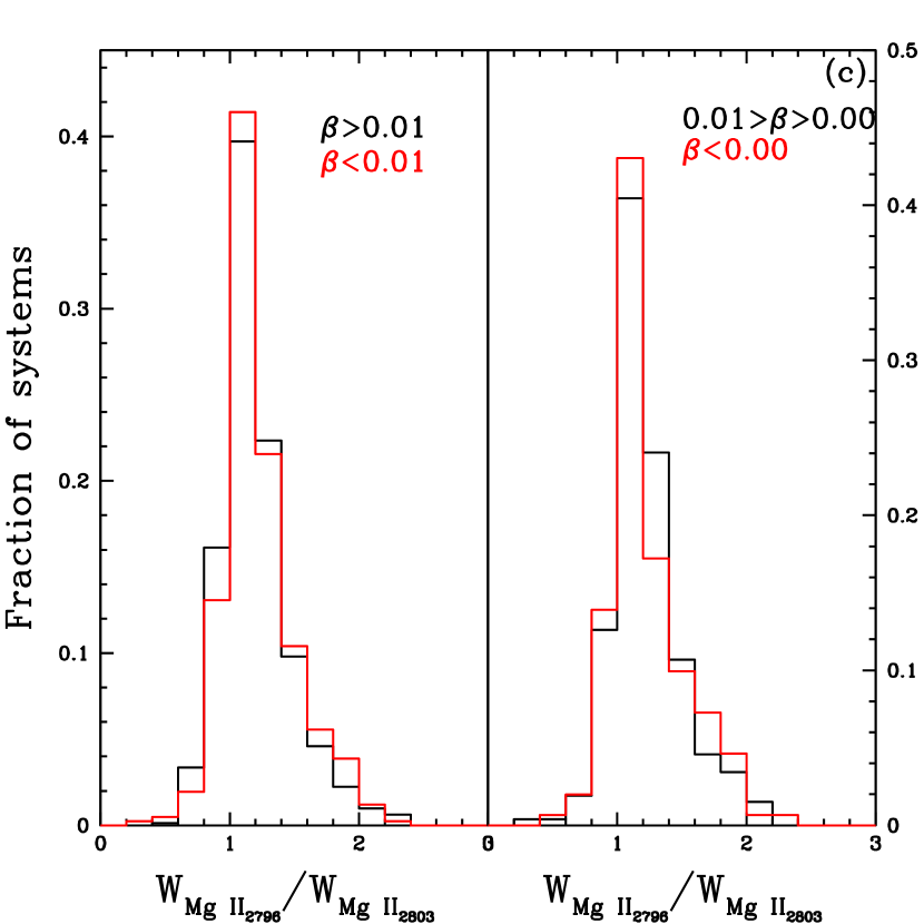
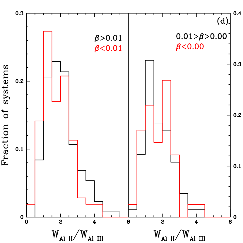
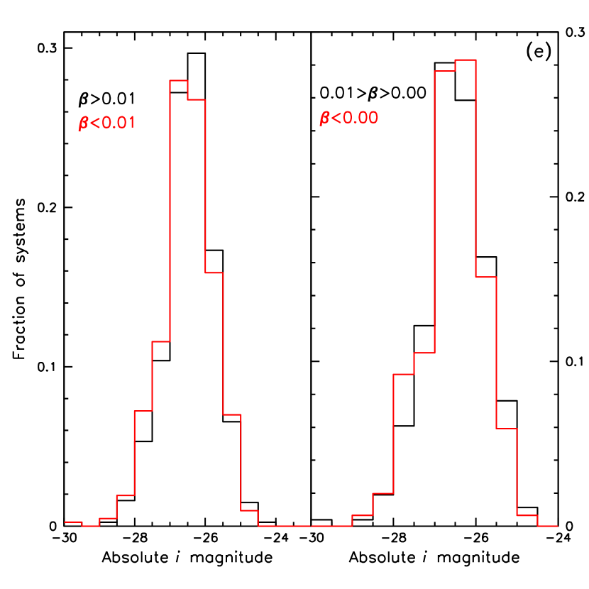
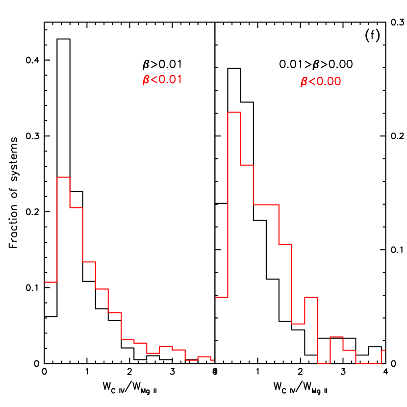
Figure 2: Histograms comparing properties of associated (sample 1, this paper, $\beta<$ 0.01, red) and intervening (SY06, $\beta>$ 0.01, black) systems appear on the left side of five sub-panels which show (a) ${\rm W}_{\rm Mg\;II}$; (b) ${\rm W}_{\rm Mg\;I}/{\rm W}_{\rm Mg\;II}$; (c) the Mg II doublet ratio; (d) ${\rm W}_{\rm Al\;II}/{\rm W}_{\rm Al\;III}$; and (e) absolute $i$ magnitude. Panel (f) shows the ratio W${}_{\rm C\;IV}$/W${}_{\rm Mg\;II}$, taken as an indicator of ionization. The left side of that panel compares the sample of associated systems (sub-sample #12, $\beta$$<$0.01, red) with the intervening systems from Y06 (sub-sample SY06CIV, $\beta$$>$0.01, black), that is the sub-samples with complete coverage of C IV doublets. The right side of panels (a) to (e) show the positive (black) and negative (red) $\beta$ associated systems from sample #1 (sub-sample #s 6 and 7) of this paper. The right side of the panel (f) shows positive (sub-sample #13, black) and negative (sub-sample #14, red) $\beta$ sub-samples for the Mg II systems from the associated systems in sub-sample #12 of this paper (complete in C IV).

To compare the properties of the associated (sample #1) and the intervening (SY06) systems, we have plotted in Figure 2 the distribution of W${}_{\rm Mg\;II}$, W${}_{\rm Mg\;I}$/W${}_{\rm Mg\;II}$, the doublet ratio of Mg II, ${\rm W}_{\rm Al\;II}/{\rm W}_{\rm Al\;III}$,  and absolute $i$ magnitudes for the two samples (left side of the Figures 2a to 2e). The ionization measure, W${}_{\rm C\;IV}$/W${}_{\rm Mg\;II}$ for the associated (#12) and intervening (SY06CIV) sub-samples is shown in the left side of Figure 2f (recall that both these sub-samples have spectra which cover both C IV and Mg II doublets). Here, W${}_{\rm Mg~{}I}$, W${}_{\rm Al~{}II}$, W${}_{\rm Al~{}III}$ and W${}_{\rm C\;IV}$ are the rest frame equivalent widths of Mg I $\lambda 2852$, Al II $\lambda 1670$, Al III $\lambda 1854$ and C IV $\lambda 1548$, respectively, in Angstroms. We use vacuum wavelengths throughout and truncate the values in our ion notation. In making these plots we have used only systems for which the equivalent widths of the lines are significant at more than the 4 $\sigma$ level. For sub-sample #12, C IV lines were below 4 $\sigma$ for 26 systems, of the 250 total systems in the sub-sample. The upper limits on W${}_{\rm C\;IV}$/W${}_{\rm Mg\;II}$ for these systems are $<$0.8. Thus they will mostly fall within the first two bins. Similarly, for the SY06CIV sub-sample, the C IV lines were not detected at 4 $\sigma$ significance for 52 systems. The upper limits on W${}_{\rm C\;IV}$/W${}_{\rm Mg\;II}$ for these systems are $<$0.5 and these systems will lie in the first two bins. We have also plotted in Figure 2, the distributions for associated systems with positive and negative $\beta$ (sub-samples #s 7 and 6 on the right of Figures 2a to 2e; sub-samples #s 13 and 14 on the right of Figure 2f).

Qualitatively, it is clear from Figure 2 that, while the distribution for two parameters: the Mg II doublet ratio and the absolute $i$ magnitude, are similar between the associated and intervening samples, those for the three ion ratios compared, and for the Mg II equivalent widths, are not. These conclusions also seem to apply to the samples with positive and negative $\beta$ values.

We have performed a number of statistical tests to determine the probabilities that the quantities plotted in Figure 2, the equivalent width of C IV $\lambda$1548, and the doublet ratio for C IV, for the intervening and associated systems, and also for sub-samples #s 7 and 6, are drawn from the same distributions. We have performed the KS test for three cases: (1) taking only the measured values of various quantities and ignoring the non-detections, (2) assuming the values for the non-detections to be zero, and (3) assuming the values for the non-detections to be equal to 3 $\sigma$ values. The actual result should be bracketed by these cases, in particular cases 2 and 3. In addition, to directly account for the upper limits we have used two commonly employed tests from survival analysis statistics, namely the Gehan and logrank tests, which are described in astronomical nomenclature by (Feigelson & Nelson 1985). Like the KS test, both survival analysis tests are designed to compare the distributions of a parameter measured in two samples; unlike the KS test, they take the upper limits within the distributions into account. Both survival analysis tests give similar results when applied to the current data sets. The results of these tests are given in Table 2. These show that the doublet ratios of Mg II and C IV, and the absolute magnitudes of associated and intervening systems are drawn from the same distributions, indicating a similar degree of saturation of the Mg II and C IV lines for these two types of systems. These conclusions are also valid for the two samples with positive and negative $\beta$ values. The equivalent width distribution for Mg II differs for the comparison of associated to intervening samples, but not for the two associated samples. The W${}_{\rm C\;IV}$/W${}_{\rm Mg\;II}$ ratios and possibly, the W${}_{\rm Mg\;I}$/W${}_{\rm Mg\;II}$ ratios for the associated and intervening systems are different, indicating a difference in ionization levels of the two types of systems; the associated systems being more highly ionized as compared to the intervening systems (see Figure 2). The situation is not so clear for W${}_{\rm Al\;II}$/W${}_{\rm Al\;III}$ ratio, for which, the KS test and the survival analysis tests give very different results.

The situation regarding dependence of ionization of $\beta$ is less clear. The results of KS tests for W${}_{\rm C\;IV}$/W${}_{\rm Mg\;II}$ and W${}_{\rm Mg\;I}$/W${}_{\rm Mg\;II}$ do indicate a difference in ionization levels; the negative $\beta$ systems being more highly ionized compared to the positive $\beta$ systems (see Figure 2). However, the survival analysis results do not corroborate this. The distribution of W${}_{\rm C\;IV}$ is however very different for the two samples.

The ratio W${}_{\rm Mg\;I}$/W${}_{\rm Mg\;II}$ is enhanced among the associated systems compared to the intervening systems, for ratios near 0.6 (SY06), evidently mainly because of the contribution of systems with $\beta$$<$ 0, so the statistical tests give low probability of the compared distributions being the same. This feature could represent an enhancement of Mg I owing to higher density in the negative $\beta$ systems, to a different temperature (affecting the recombination rate of Mg I; York & Kinahan 1979) or to a specific effect of the ionization field near 1100 Å (the ionization limit of Mg I). (It was found by Y06 that the blend of components that constitutes the Mg I feature typically technically saturated at W$\sim$0.6 Å, which could be related to the excess seen here.)

3.2 Line strengths in the composite spectra

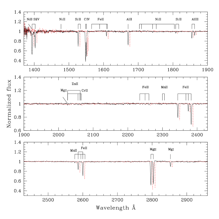
Figure 3: The arithmetic mean composite spectrum of the systems in the sub-sample (#12) of associated systems having $z_{abs}$$>1.4675$ (so that the SDSS spectrum includes the C IV doublet) in the absorber rest frame (black, solid line). Individual spectra have been normalized using the first 30 eigenspectra of the principle components of the QSO spectra and weighted by inverse variance. All spectra contribute to the region between 1540 and 3150 Å which, therefore, has high signal-to-noise. The similar spectrum for intervening absorbers (sub-sample SY06CIV, red, dotted line) culled from SY06 is shown for comparison. This spectrum is shifted by 5 Å to the right for ease in visual comparison. Please note the different y-axis scale in the middle panel. The wavelength scale is uniform, so lines of a given velocity width appear broader at longer wavelengths.

Equivalent widths of the measured lines in the arithmetic mean composite spectrum for the full sample (#1) are given in column 4 of Table 3. Also given, in column 5, are the equivalent widths of the lines for the sample of intervening systems (SY06) as obtained by Y06. To the left are the vacuum wavelengths, the species and the intrinsic strength indicator: $f\lambda^{2}/10^{4}$. While the equivalent widths of Mg II $\lambda\lambda$2796,2890 and Al II $\lambda$1670 lines are similar, the C IV $\lambda\lambda$1548,1550, Si IV $\lambda\lambda$1396,1402 and Al III $\lambda\lambda$1854,1862 (marginally) lines are stronger in the associated sample than in the intervening sample. However, as noted above, because of the selected range of $z_{em}$, the composite spectrum gets a contribution from all absorbers only for lines with rest-frame wavelength in the range 1900-3150 Å. All the systems in sub-samples #12 and SY06CIV, by construction, contribute to the composite spectrum between wavelengths 1540 and 3150 Å. The equivalent widths of various lines for these two sub-samples are given in columns 6 and 7 of Table 3. The arithmetic mean composite spectra of the two sub-samples is shown in Figure 3. It can be seen that the higher ionization C IV lines are indeed stronger and the lower ionization lines (Mg II, Fe II, Al II, Si II) are weaker in the associated systems as compared to those in the intervening systems, consistent with the earlier conclusion that the ionization is higher in associated systems.

In order to determine if the ionization level in associated systems depends on $\beta$, we measured the equivalent widths of lines in the composite spectra of sub-samples #13 and 14. These are also given in Table 3, columns 8 and 9, respectively. There is definite evidence of higher ionization for lower $\beta$ values. The average absolute $i$ magnitudes of these two sub-samples (-26.76 and -26.86 for #13 and 14 respectively) differ only by 0.1 and the distribution of absolute $i$ magnitudes is similar (KS test probability that they are drawn from the same distribution being 0.13), so that the difference in ionization is not caused by different intrinsic ionizing fluxes of the QSOs.

It has been found that, in a few QSOs, the absorbing material giving rise to the associated systems covers the continuum source in the QSO only partially (e.g. Barlow & Sargent 1997; Hamann et al. 1997b). This can complicate the interpretation of the observed equivalent widths. The partial coverage of the source will change the doublet ratios of the absorption lines. The two lines of the C IV doublet are not completely resolved (detached) in our composite spectra. However, the distributions of the doublet ratios of Mg II lines for the intervening and associated samples, as well as the sub-samples with different $\beta$ ranges are very similar (see Figure 2 and Table 2). The equivalent widths and line profiles of Mg II lines in sample #1 and SY06 are also very similar. So the issue of covering factor may not be very important. Also, the equivalent widths of lines of C IV and Mg II differ in opposite senses in sub-samples with different $\beta$ values. Thus we believe that our interpretation of higher ionization in associated absorbers as compared to the intervening systems and its dependence on $\beta$ in associated absorbers is justified.

The strongest lines in Figure 3 undoubtedly consist of many components, some saturated and some not. To understand the detailed behavior of the composite spectra will require high resolution observations of a number of individual systems, to fully sort out the effects of saturation, any dilution by low covering factors that may exist in some cases and blending of many components. Such a program has already been undertaken for the intervening sample (Meiring et al. 2006; Peroux et al. 2006): differences between that sample and an associated sample observed in the same way will be very useful for understanding the associated systems. However the global ionization effects noted here, from equivalent width ratios of the strong lines (of C IV and Mg II), which show consistent behavior among various sub-samples, should not change.

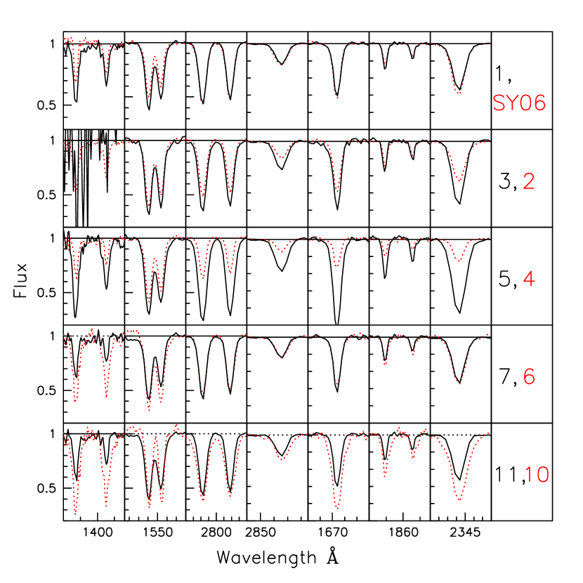
Figure 4: Comparison of profiles of absorption lines Si IV $\lambda\lambda 1393,1402$, C IV $\lambda\lambda 1548,1550$, Mg II $\lambda\lambda 2796,2803$, Mg I $\lambda$2852, Al II $\lambda$1670, Al III $\lambda\lambda$ 1854,1864 and Fe II $\lambda$ 2344 in the arithmetic mean composite spectra of sub-samples. Sample numbers are given in the rightmost panels. Selection criterion of the samples (as given in Table 1) are briefly described below for ease in comprehension. The pairings are, with the samples plotted and labeled in red given first, SY06, #1: full samples of intervening and associated absorbers; #2, 3: $i\;{\rm magnitude}$$<$ and $\geq$ 18.74; #s 4, 5: ${\rm W}_{\rm Mg\;II}$$<$ and $\geq$ 1.35 Å; #s 6, 7: $\beta$$<$ and $\geq$ 0; #s 10, 11: Radio-detected and undetected QSOs.

In Figure 4, we show profiles of a few selected lines in various sub-samples of associated systems. It can be seen that most lines are stronger in the sub-sample comprised of intrinsically faint QSOs (#3) as compared to those in the sub-sample comprised of intrinsically bright QSOs (#2) (the average observed $i$ magnitudes for the two sub-samples also differ considerably). This was also observed by Y06 for the intervening systems and was understood as being the effect of lower S/N ratio in the spectra of faint QSOs, which makes only relatively stronger absorption systems in these QSOs detectable at the 4 $\sigma$ level. As expected, all the lines are stronger in the sub-sample of stronger Mg II systems (#5) as compared to those in the sub-sample of weaker Mg II systems (#4). As noted above, lines of higher ionization are stronger in the sub-sample (#6) of smaller $\beta$ compared to those in the sub-sample (#7) of larger $\beta$ values. Finally, all of the lines are stronger in the sub-sample (#10) of RD QSOs as compared to those in the sub-sample (#11) of RUD QSOs. This appears to be due to the fact that sub-sample #10 is comprised of stronger Mg II systems, having average W${}_{\rm Mg\;II}$ = 1.9 Å compared to 1.52 Å for sub-sample #11. One of the systems in sub-sample #10 has very high ${\rm W}_{\rm Mg\;II}$($\sim$ 9 Å). This contributes significantly to the equivalent widths of most lines in the composite spectrum of the sub-sample.

The strong ionization effect noted in C IV is even more noticeable in Si IV (Table 3, Figure 3 and Figure 4, row 4). This could be an effect of just a few, peculiar systems with high enough redshift to contribute to both sample #s 1 and 12. To check this, we formed a sample of systems with $z_{abs}$$>$ 1.7378, so that Si IV was completely covered in all cases, along with C IV and Mg II. The same trends evident in Table 3 persist. For respective sub-samples of (a) intervening systems (from Y06); (b) associated, positive $\beta$ systems; and (c) associated, negative $\beta$ systems, all with $z_{abs}$$>$1.7378, the values of the equivalent widths of Si IV $\lambda$1393 are 380, 590 and 1330 mÅ, while for W${}_{\rm C\;IV}$ we find 880, 1060 and 1320 mÅ, respectively. These values are within 10% of the corresponding number from sub-samples 12, 13 and 14 in Table 3, so the effect does seem to be real. That is, the Si IV lines are relatively stronger as the systems have lower and lower $\beta$s. The number of systems in these sub-samples are only 35, 27 and 45, so this result needs to be confirmed in much larger samples (e.g., SDSS DR5).

3.3 Extinction

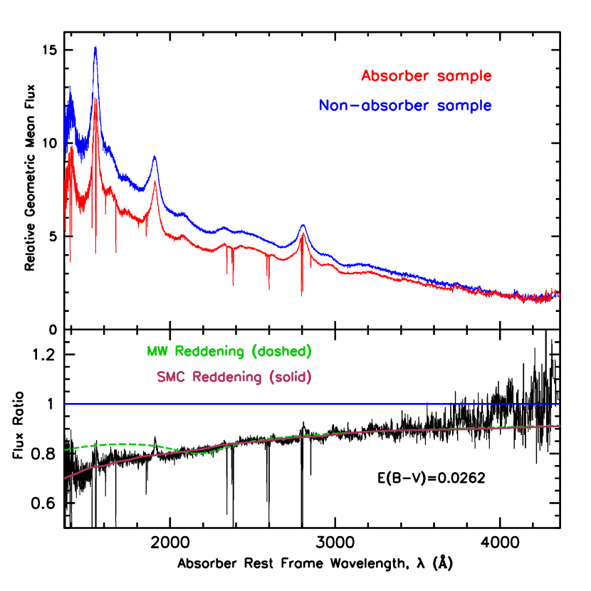
Figure 5: The top panel shows the geometric mean composite spectrum of the QSOs in sample #1, in the absorber rest-frames, in red, and that of the corresponding non-absorbers, in blue. Note that emission lines do appear in the absorber rest-frame composite spectrum due to the small difference in emission and absorption redshifts of the QSOs in the sample of associated systems. The absorption lines in the red spectra are obvious. See text for a discussion of the normalization of the plots. The bottom panel shows the ratio of the two spectra along with the best fit SMC extinction curve in red. The derived absorber rest frame $E(B-V)$ value is given. The MW extinction curve for the derived SMC $E(B-V)$ value is shown in green.

The geometric mean composite spectrum for the full sample (#1) is given in Figure 5. Also plotted is the composite spectrum for the matching non-absorber sample. In the bottom panel of the Figure we have plotted the ratio of the two composites, the best-fit SMC extinction curve, and the Milky Way extinction curve for the same value of $E(B-V)$. Similar to the case of intervening systems (Y06), no 2175 Å bump is seen in the observed spectrum. The bump is not present in the composite spectrum of any of the sub-samples either, and the SMC extinction curve appears to describe the observed extinction curve reasonably well. This is also supported by the fact that the $E(B-V)$ values are close to 0.25 times the average values of $\Delta(g-i)$ for the sub-samples (see Table 1). Such a relationship was discovered by Y06 for the sub-samples of intervening systems, which also seemed to be well described by an SMC type of extinction curve. The lack of evidence for a significant 2175 Å bump is consistent with the fact that the feature has been detected in the spectra of only a small number of individual QSOs (e.g. Motta et al. 2002; Wang et al. 2004; Junkkarinen et al. 2004; Mediavilla et al. 2005, see additional comments in Y06).

By contrast to the case of intervening systems (Figure 2 of Y06 for instance), the composite spectra for the associated systems (top panel of Figure 5 in this paper) show typical QSO emission lines. This is due to the fact that for associated systems, the absorption redshifts are very close to the emission redshifts and the emission lines in individual spectra are very nearly aligned even in the absorber rest-frames. In the extinction curves (in the bottom panel), there appears to be some emission present at the wavelengths of [C III] and Mg II lines and possibly those of other QSO emission lines. This could be due to either the emission by the absorbers, or an artificial effect produced by the small differences in the emission redshifts of the absorber and non-absorber QSOs. From Figure 5 one also gets the impression that the shape of the emission lines in the absorber and non-absorber spectra are different. In order to understand these effects we produced geometric mean composite spectra of the absorber and non-absorber samples in the rest frame of the QSOs. The ratio of these two composites did not show any emission. This shows that the emission line profiles in the QSOs with associated absorbers and QSOs without associated absorbers are, on average similar in shape. This possibly also indicates that the emission seen in the extinction curves of Figure 5 is not real and is the effect of the difference in the emission redshifts of the absorber and non-absorber QSOs. We can not however completely rule out emission from the absorbers.

About 28% of the QSOs in sample #1 also have other, intervening, absorption systems in their spectra. These, in principle, could contribute to the values of $E(B-V)$ determined here. The effect is likely to be small in view of the results of Y06, which showed that intervening systems with W${}_{\rm Mg\;II}$ smaller than 1.53 Å do not produce significant reddening and far outnumber the systems with stronger Mg II absorption that do produce reddening. However, to evaluate the effect of these intervening systems, we constructed composites for the sub-sample of 298 associated systems (from our sample #1) which had no other absorption systems in their spectrum. The $E(B-V)$ for this sub-sample is 0.029$\pm$0.003, which is the same as that of Sample #1, to within the errors. We thus conclude that the other systems in 117 QSOs in our sample #1 are too weak to affect the value of $E(B-V)$ due to associated systems determined here.

The extinction for the full sample (#1; $E(B-V)$=0.026$\pm$0.004) is twice that obtained for the intervening sample (SY06; $E(B-V)$=0.013), indicating a higher amount of dust in the associated systems. This could partly be due to the following reason. As noted in the last sub-section, the ionization level is higher in the associated systems. Thus, by choosing systems with W${}_{\rm Mg\;II}$ $>0.3$ Å, we have possibly chosen the associated systems with higher total Mg column (that is, including all ionization states) and thus higher total hydrogen column and therefore, higher dust column as compared to those in the intervening systems. We note that the average W${}_{\rm Mg\;II}$ in the intervening systems (1.73 Å) is higher than that in the associated systems (1.54 Å). This could be due to the ionization effect mentioned above. It is however, not clear if the higher $E(B-V)$ in the associated systems is due to this effect alone. It is possible that the associated systems have higher dust-to-gas ratio. It is also possible that part of the reddening is caused by the dust intrinsic to the QSO, but not containing Mg II (because of ionization?). As shown in the next sub-section, the reddening is strongly dependent on the radio properties of the QSOs. We return to these points, below.

The extinction in the sub-sample of faint QSOs (#3) is somewhat higher than that in the sub-sample of bright QSOs (# 2). The average W${}_{\rm Mg\;II}$ for the fainter sub-sample is higher (1.70 Å) compared to that for the brighter sub-sample (1.37 Å). This possibly indicates that the fainter QSOs are fainter because of the higher dust content of the DLAs lying in front of them. In the sub-sample of systems with W${}_{\rm Mg\;II}>1.35$ Å (#5) it is close to two times that in the sub-sample of systems with W${}_{\rm Mg\;II}<1.35$ Å (#4). Surprisingly, the value of $E(B-V)$ is 1.5 times higher in associated systems with negative $\beta$ (#6) than those with positive $\beta$ (#7). Note that both these sub-samples have similar values of W${}_{\rm Mg\;II}$. As noted in the previous sub-section, the ionization seems to be higher in sub-sample #6 than in sub-sample #7. The higher amount of dust may thus indicate higher amount (by a factor $\sim$ 1.5) of the total hydrogen (neutral plus ionized) in the latter. A similar dependence of $E(B-V)$ on $\beta$ is observed if we divide the positive $\beta$ sub-sample (# 7) into two halves at the median value of 0.004. The lower $\beta$ sub-sample has $E(B-V)$ which is higher than that of the high $\beta$ sub-sample. The effect is also seen in sub-sample #s 13 and 14. Thus the $\beta$ values seem to be an indicator of the state of ionization of the absorbers and of the amount of reddening. Similar effects have been noted by Baker et al. (2002) and V03 using less quantitative means. The effect found here is much more subtle that that claimed by Baker et al. (2002). The effect of radio properties of the QSOs on the extinction is discussed in the next sub-section.

3.4 Dependence on radio properties of QSOs

In our sample of the associated systems, 48 QSOs have non-zero FIRST flux (the RD sub-sample, #10) while 318 QSOs have non-detection in the FIRST survey (the RUD sub-sample, #11); the rest have not been observed by the FIRST survey. (Hereafter, we drop reference to the FIRST survey, which is implied when we refer to radio sources.) In the SDSS DR3, the number of QSOs with $z_{em}$ between 1 and 1.96 is 23,914, in all of which we could have seen associated Mg II absorbers if present. Of these 1,728 are RD and 19,056 are RUD (the rest have not been observed by the FIRST survey). As the selection criterion for the RD and RUD sub-samples (as described in section 2.1) were identical and because the average observed $i$ magnitudes (18.60 and 18.63 for the RD and RUD sub-samples respectively), the average absolute $i$ magnitudes (-26.35 and -26.52 for the RD and RUD sub-samples respectively) and $z_{abs}$ (1.39 and 1.5 for the RD and RUD sub-samples respectively) of the two sub-samples are almost equal, no other biases are present and we can compare the frequency of occurrence of these systems. Thus the incidence of associated absorbers with ${\rm W}_{\rm Mg\;II}$$>$ 0.3 Å in RD QSOs is 2.8% while that in RUD QSOs is 1.7%. RD QSOs are thus 1.7 times more likely to have associated absorption as compared to the RUD QSOs. Assuming binomial statistics, the probability of getting such a large difference in the incidence of associated systems between the two sub-samples is less than 1%.

3.4.1 Intrinsic redness of radio-detected QSOs

As can be seen from Table 1, the reddening in the RD QSOs with associated Mg II systems is five times higher than that in the RUD QSOs. As noted in section 1, associated C IV absorption may occur preferentially in steep-spectrum radio sources. If, as is often assumed (see section 1), such sources are viewed in the edge-on position, it is possible that the material in the accretion disc/torus (unrelated to the absorption systems) may be causing part or even most of the observed reddening in the radio-loud QSOs. The ‘redness’ of radio QSOs has been noted earlier (e.g. Brotherton et al. 2001; Baker et al. 2002; Ivezic et al. 2002).

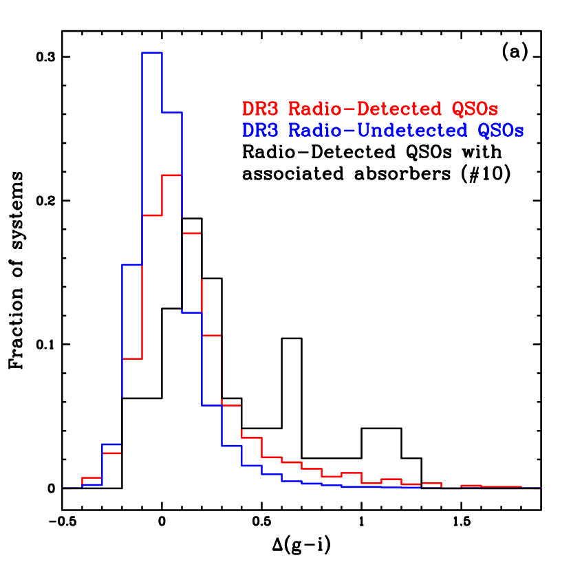
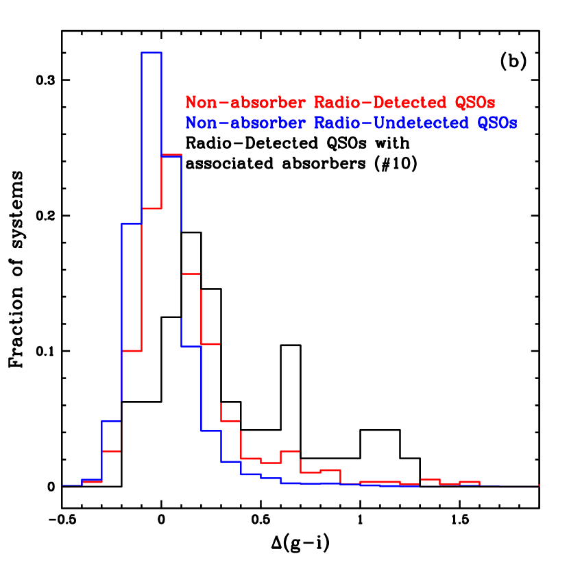
Figure 6: The left panel (a) shows the distribution of $\Delta(g-i)$ in SDSS DR3 QSOs with $1.0<z_{em}<1.96$, having (i) non-zero FIRST flux (red) and (ii) non-detection in the FIRST survey (blue). Also shown is the distribution for FIRST radio-detected QSOs in our sub-sample (#10) of associated systems (black). The right panel (b) shows the distribution of $\Delta(g-i)$in SDSS DR3 QSOs with $1.0<z_{em}<1.96$, confirmed by the present study as having no absorption systems in their spectra and having (i) non-zero FIRST flux (red) and (ii) non-detection in the FIRST survey (blue). Also shown is the distribution for FIRST radio-detected QSOs in our sub-sample (#10) of associated systems.

To investigate this, we have, in Figure 6a, plotted histograms of $\Delta(g-i)$ of all RD (red lines) and RUD (blue lines) QSOs with $1.0<z_{em}<1.96$ (which is the emission redshift range of our sample of associated absorbers) in the DR3 catalog (Schneider et al. 2005). It can be seen that the RD QSOs have a higher fraction of red QSOs as compared to that in RUD sample (the red histogram is shifted to the right). As many of the QSOs in the DR3 RD and RUD sub-samples may have absorption systems, we have in Figure 6b, plotted similar histograms for RD and RUD sub-samples of non-absorber DR3 QSOs having $z_{em}$ between 1 and 1.96. There are 580 RD non-absorber QSOs (red lines) in this redshift range while there are 6,786 RUD non-absorber QSOs (blue lines). According to Y06, unreddened, unabsorbed QSOs have -0.2$<\Delta(g-i)<$ +0.2, consistent with the RUD, non-absorber QSOs plotted in Figure 6b. The RD, non-absorber QSOs have a much larger fraction of red QSOs as compared to the RUD non-absorber sample. Thus, we have definite evidence of RD QSOs being intrinsically redder than the RUD QSOs.

In order to quantify the intrinsic redness of the RD, non-absorber QSOs, we constructed a composite spectrum of 250 RD, non-absorber QSOs in the QSO rest-frame and compared it with similar composite spectrum of matching (in $i\;{\rm magnitude}$ and $z_{em}$) 250 RUD, non-absorber QSOs. The KS test shows that the $i\;{\rm magnitude}$ and $z_{em}$ values in the two sub-samples are drawn from the same distributions. The composite spectrum of the RD non-absorber QSOs is redder than that of RUD non-absorber QSOs. An SMC extinction curve gives a good match to the ratio of the two composites yielding a relative $E(B-V)$= 0.036$\pm 0.0001$, as the intrinsic average color excess in RD QSOs over RUD QSOs (see Table 4).

3.4.2 Dependence of extinction properties of associated absorbers on the radio properties of QSOs

To test whether the higher $E(B-V)$ in RD QSOs is solely because of the intrinsic dust in these QSOs or if the associated absorbers in these QSOs also have higher dust content as compared to the rest of the associated absorbers, we have in Figures 6a and 6b plotted the histograms of $\Delta(g-i)$ (black lines) for the sub-sample #10. It is clear that the RD QSOs with associated absorbers have a higher fraction of red QSOs as compared to the RD non-absorbers (the black histograms extend more to the right). Thus the RD QSOs with associated absorbers are more likely to be reddened as compared to those without such absorbers. While 56% of RD QSOs with associated absorbers have $\Delta(g-i)$$>$0.2, the numbers for the RD and RUD non-absorber QSOs (with $z_{em}$ between 1 and 1.96) are 26% and 8% respectively. The three numbers for $\Delta(g-i)$$>$0.5 are 31%, 9% and 1.6% respectively. Evidently, studies of extinction in radio QSOs must consider whether associated absorbers are present or not, especially in individual cases.

In order to quantify this result further, we compiled a matching sample of QSOs (for the absorber QSOs in sub-sample #10) from among the RD non-absorber QSOs. The resulting $E(B-V)$ was found to be 0.062$\pm 0.007$ (see footnote d in Table 1), smaller than the $E(B-V)$ of sub-sample #10 in Table 1 by a factor of only 1.4, showing that though the RD, non-absorber QSOs are redder than the RUD, non-absorber QSOs, a significant fraction of the reddening in our sub-sample of RD QSOs is caused by the dust in the associated absorbers.

As noted in section 3.2, the average W${}_{\rm Mg\;II}$ of the RD sub-sample (#10, 1.9 Å) with associated Mg II absorbers is higher than that of the full sample (#1, 1.54 Å). Although, higher ${\rm W}_{\rm Mg\;II}$ is likely to be indicative of a larger velocity dispersion of Mg II lines, a correlation between $E(B-V)$ and ${\rm W}_{\rm Mg\;II}$ has been noticed by Y06 and is also seen in our sample (see sub-sample #s 4 and 5 in Table 1). Thus, the higher W${}_{\rm Mg\;II}$ of the RD sub-sample could be partially responsible for the higher $E(B-V)$. However, we note that the $E(B-V)$ for the RD sub-sample (#10) is much higher than for the sub-sample (#5) of strong systems for which the average W${}_{\rm Mg\;II}$ is 2.23 Å but $E(B-V)$ is only 0.034$\pm$0.003. Thus, the somewhat higher average W${}_{\rm Mg\;II}$ for the RD sub-sample compared to the RUD sub-sample is not the sole reason for the high value of $E(B-V)$ which is definitely related to the QSOs being RD.

If a large part of the excess extinction, observed in RD QSOs (over RUD QSOs), is generated in the associated absorbers, then the $E(B-V)$ values in these QSOs will depend on the absorber properties. In order to investigate this issue, we divided the sub-sample of RD QSOs (#10) into two parts, at the median value of W${}_{\rm Mg\;II}$ of 1.58 Å. The relative $E(B-V)$ value of the high W${}_{\rm Mg\;II}$ sub-sample with respect to the low W${}_{\rm Mg\;II}$ sub-samples (obtained by fitting an SMC extinction curve to the ratio of the composite spectra of the two sub-samples) is 0.092$\pm 0.003$. Division into three equal parts based on W${}_{\rm Mg\;II}$ (W${}_{\rm Mg\;II}<$ 1.22, 1.22$<$W${}_{\rm Mg\;II}<2.1$ and W${}_{\rm Mg\;II}>$2.1 Å) gives relative $E(B-V)$ (obtained as explained above ) = 0.074$\pm 0.001$ and 0.053$\pm 0.001$ for the two pairs of neighboring sub-samples (the higher W${}_{\rm Mg\;II}$ sub-samples being redder). The values of relative $E(B-V)$ are given in Table 4. It is clear that the $E(B-V)$ is correlated with ${\rm W}_{\rm Mg\;II}$. The Spearman rank test to determine the presence of a correlation between W${}_{\rm Mg\;II}$ and $\Delta(g-i)$ gives $R_{s}$ = 0.463 and the probability of chance correlation to be 0.001. Thus it is very clear that the higher reddening in the RD QSOs with associated absorbers is strongly correlated with the strength of Mg II absorption lines and should, therefore, be due to the dust present in the absorbers. The fact that RD QSOs are intrinsically redder, evidently harboring more dust in their associated systems (as compared to that in the systems associated with the RUD QSOs) may indicate that the absorbing material is similar to that in the QSO and may thus be intrinsic to the QSO. We do not, however, find any evidence of enhanced abundances in the composite spectra (as in Figure 3) as discussed in section 3.5 below.

3.4.3 Comparison with the intervening sample

A significant contribution to the $E(B-V)$ value for the full sample (#1) must come from the RD QSOs. For forty-nine objects in that sample, no radio observations are available. Some of these could also have significant radio flux. The RUD sub-sample (#11) has $E(B-V)$ of 0.016$\pm$0.004. The QSOs in the matching non-absorber samples for these do have some RD QSOs, so the value of $E(B-V)$=0.016 is a lower limit. Restricting the non-absorber sample to RUD QSOs we get $E(B-V)$=0.018$\pm$0.0007 (see Table 1 footnote e). We have to compare these values with $E(B-V)$ values for similarly selected sub-samples of the intervening systems (SY06). Forty one systems in SY06 have been detected by the FIRST survey while 614 are RUD; the remaining 129, have not been observed by the FIRST survey. To avoid effects due to the selection of matching non-absorber sub-samples, instead of determining the absolute $E(B-V)$ values for these sub-samples, we directly determine relative $E(B-V)$ values between the RD and RUD, intervening and associated sub-samples by fitting an SMC extinction curve to the ratio of composite spectra of the sub-samples being compared. We find that the RD associated systems have a relative $E(B-V)$ of 0.062$\pm 0.0001$ with respect to the RD intervening systems. The RUD associated systems have a relative $E(B-V)$ of 0.018$\pm 0.001$ with respect to the RUD intervening systems. Thus the RD QSOs with associated absorbers are definitely more reddened as compared to the RD QSOs with intervening absorbers. The RUD QSOs with associated absorbers are also more reddened as compared to the RUD QSOs with intervening absorbers. Thus on the whole, the associated absorbers are dustier than the intervening absorbers. Relative values of $E(B-V)$  among several sub-samples are given in Table 4.

3.4.4 SDSS color-selected-radio-detected QSOs

As noted in section 2.1, SDSS QSOs are mostly color selected, but some QSOs (particularly those below $i$ magnitude of 19.1) are selected because of their being ROSAT or FIRST sources. Such sources may be be redder than the average because they may not satisfy the SDSS color-selection criteria, but instead have colors consistent with the stellar locus. It is possible that the presence of such sources in the RD sample (#10) may be responsible for the excess reddening in this sub-sample. Ten sources in sub-sample #10 are not color-selected while 2 of the RD QSOs in SY06 are not color-selected. The relative $E(B-V)$  of the sub-sample of color-selected RD QSOs with associated systems with respect to the color-selected RD QSOs with intervening systems (see Table 4) is 0.048$\pm 0.0001$ (compared to 0.062 when the non-color selected QSOs are included). Thus, the color-selected RD QSOs with associated absorbers are significantly redder than the color-selected RD QSOs with intervening absorbers.

3.4.5 Radio Morphology

As noted above, the presence of associated absorbers in radio QSOs may be correlated to the morphology and radio spectral slope of these QSOs. Outflows from QSOs (e.g. jets or accretion disk winds) can give rise to associated systems (e.g., Richards et al. 2001; Misawa et al. 2007). Models using beamed radio jet emission have been proposed to unify flat-spectrum radio quasars and steep-spectrum radio galaxies (e.g., Orr & Browne 1982; Padovani & Urry 1992). On average, a flat-spectrum quasar is thought to be viewed closer to the jet axis than a steep-spectrum quasar. Here we examine the radio morphologies and spectral indices of quasars with and without associated absorption with the hope of understanding the connection between the direction of motion of the outflow (e.g. polar or equatorial) and the absorber properties.

To study the radio morphology of quasars in our sub-samples, we proceeded as follows: For each of the 48 RD quasars with associated absorbers (sample #10), we searched for sources detected in the FIRST image within 1.0’ of the quasar’s optical (SDSS) coordinates. (At $1<z<2$, an angular separation of 1’ corresponds to about 500 kpc for the concordance cosmology.) First, we visually examined the morphologies in the FIRST images. If the source was clearly resolved as a multi-component source (i.e., at least 1 distinct source besides the core was found within about 30”), then we considered the source a lobe (“L”) source. If a single source, without a counterpart on the other side, was found between 30” and 60” from the core, then it’s likely not related to the quasar, and we treated the quasar as a core (“C”) source, rather than a lobe source. For the objects with no other source found within 60” of the core, we quantified the morphology using the procedures of Richards et al. (2001) and Ivezic et al. (2002). For each source, the FIRST catalog lists the peak and integrated flux densities. Using these, we determined a dimensionless measure of concentration of radio emission,

$$\theta=\large({F_{\rm int}\over{F_{\rm peak}}}\large)^{1/2}$$ (1)

We classified the single sources with log $\theta^{2}\leq 0.1$ as core-dominated (“C”) and those with log $\theta^{2}>0.1$ as partially core-dominated (“PC”) sources. (In a few “C” cases, the values of log $\theta^{2}$ are slightly negative due to the uncertainties in the FIRST flux measurements.) Finally, we checked that the above quantitative divisions between “C” and “PC” are consistent with the contour maps of the FIRST images. (For only one “C” source in the absorber sample, large-scale artifacts in the FIRST data give rise to log $\theta^{2}>0.1$.) With these definitions, the 48 quasars in sample #10 consist of 26 “C”, 8 “PC”, and 14 “L” sources. Thus, $46\%$ of the sources in the absorber sample are spatially resolved (“PC” or “L”-type).

To understand how far these fractions relate to the existence of an associated absorber along the sightline, we repeated the above procedure for the matching 48 RD quasars with no absorbers. Of these 48 quasars, 31 are “C” sources, 6 “PC” sources, and 11 “L” sources. Thus, 35 $\%$ of the sources in the non-absorber sample are spatially resolved. There is thus a slight excess of spatially resolved sources in the absorber sample compared to the non-absorber sample. Using binomial statistics, the probability of finding a fraction of $46\%$ or more resolved sources in the absorber RD sample, if the true fraction is only $35\%$, is about $0.08$. Thus the difference between the samples is not highly significant. To confirm such an excess at the $1\%$ level would require a sample size of about 100 objects, which should be possible to construct from the SDSS DR5 QSO data set.

We constructed absorber rest-frame composite spectra of the 26 “C” QSOs and of the 14 “L” QSOs. As the line of sight to the “L” QSOs is expected to pass near or through the accretion disc, these QSOs are expected to be more reddened. However, we find that the “C” composite is redder than the “L” composite, the relative $E(B-V)$ being 0.042. This could very well be a small sample effect and it will be very interesting to repeat this for bigger samples.

It is not possible to determine radio spectral indices for all of the quasars in the RD absorber and non-absorber samples, since flux densities at wavelengths other than 20 cm are not available for most of them. Of the 48 RD quasars with associated absorbers, only 15 have measurements at other wavelengths [14 from the Green Bank (GB) 6 cm catalog (White & Becker 1992), and one at 80 cm]. Using these along with the 20 cm FIRST measurements, we calculated the spectral indices. (In a few cases, the spectral index based on the GB and FIRST measurements is somewhat different from that listed in White & Becker (1992), which probably results from different resolutions of the two surveys and possible variability between the two epochs of observation.) In any case, taking the spectral index $\alpha_{\rm int}$ thus calculated using integrated flux densities, we classified objects as flat-spectrum (“F”) if $|\alpha_{\rm int}|\leq 0.4$ and steep-spectrum (“S”) otherwise. Of the 15 quasars in the absorber sample where we could determine $\alpha_{\rm int}$, eight are “F” sources. Of the seven steep-spectrum sources, five have log $\theta^{2}\leq 0.10$ and are thus likely to be compact. This suggests that these associated absorbers are associated with outflow material located close to the polar direction. In the non-absorber sample, 6 cm fluxes are available for seven quasars, of which four are steep-spectrum sources (including one compact steep-spectrum source). Thus compact steep-spectrum sources may be more common in cases with associated absorbers.

Overall, some fraction of the associated absorbers appear to arise in material along the polar axis, while others arise in material away from the polar axis. Larger samples are needed to study systematically correlations among the absorber properties and outflow orientation and line-of-sight velocity.

3.5 Abundances

There seems to be wide agreement that the abundances in the broad emission line regions are super-solar (Ferland et al. 1996; Hamann & Ferland 1999; Hamann et al. 2002; Baldwin et al. 2003; Nagao et al. 2007; Dhanda 2007) (and the same is true for the narrow line regions of Seyfert 2 galaxies; Groves et al. (2006)). There are a number of instances of suspected super-solar abundances in associated absorbers (D’Odorico et al. 2004, Hamann 1997, Petitjean et al. 1994, Tripp et al. 1996). Fu & Stockton (2006) discuss the contamination of the broad line region and EELR by mergers with galaxies with sub-solar abundances.

It can be seen from Table 3 that for the weakest lines of dominant ions of Mn (3 lines near 2600 Å), Fe ($\lambda\lambda$2260, 2249), Cr (3 lines near 2062 Å) and Zn ($\lambda\lambda$2026, 2062), the ratios of lines of each species indicate that the weakest lines are on the linear portion of the curve of growth, independent of the Doppler widths or the width or saturation of the stronger lines. We assume that Si II $\lambda$1808 is on the linear portion of the curve of growth. (Note that the relative strengths of $\lambda$1808 and $\lambda$1526 indicate that the Doppler width, in this case related to the spread of components, is probably somewhat higher in sample #1 than in sample SY06, making our assumption conservative.) Then, the equivalent widths of the weakest lines of these species are proportional to the column densities. We find that the equivalent widths of the weakest lines of these ions are weaker in sample #1 (associated system average) than the lines of the intervening averages (SY06): the ratios (sample #1 divided by SY06) are 0.8, $<$ 0.8, 0.9, 1 and $<$ 0.8 for Si II, Cr II, Mn II, Fe II and Zn II, respectively. The value for Zn II accounts for the fact that we can not deblend the Cr II 2062 line in sample #1 as we could in the SY06 sample. On the other hand, the same ratio for Ni II might be as high as 5 for the weakest line, but of order 1.4 for two other lines of comparable strength.

The extinction is twice as high in sample #1 ($E(B-V)=$0.026) as in SY06 (0.013). If the ratio of $E(B-V)$ to ${\rm N}_{\rm H\;I}$ value is the same in associated and intervening systems, then the abundances in sample #1 are slightly less than in SY06. There is no evidence that the associated systems containing Mg II have greatly enhanced abundances that would indicate an association of the associated systems with the gas from the QSO emission line region.

Of course, the dust might be different in the two types of systems, but the extinction curves are of the same general shape. There could be ionization corrections that would modify this indication about abundances: high resolution observations and analysis with CLOUDY, as shown, for instance, by Meiring et al. (2007), will be required to search for a stronger statement about the abundances. Higher resolution is needed to resolve the individual components in the systems and to resolve the contrary indication from the one result for Ni II.

Thus, from our results there is no strong effect averaged over 415 associated absorbers studied here that would indicate a relation of those absorbers to gas originating in the broad line regions.

3.6 Location and nature of the absorbers

We find several suggestions of where the associated absorbers may be coming from. First, the ionization effects in Si IV, C IV and Mg II and their dependence on $\beta$ indicate that lower $\beta$ systems are closer to the QSO. The various suggestions referenced above that place some of the associated systems in the EELR, and the confirmed existence of negative $\beta$ systems may be related to the large widths (400 ${\rm km\;s}^{-1}$) (Fu & Stockton 2006) and bigger shifts (1800 ${\rm km\;s}^{-1}$ to -600 ${\rm km\;s}^{-1}$) of emission lines in the EELR (Christensen et al. 2006). While these do not quite add up to negative $\beta$ values of –0.004 found here, the sample of EELR is small: a larger sample may show that a wider range exists, comparable to that seen in our Mg II absorbers. An extensive study of the associated systems found here, at high resolution, to determine abundances and populations of fine structure excited states is in order.

We also note the anomaly in Mg I absorption line strengths mentioned earlier. Hamann et al. (2001) found relatively strong Mg I lines in the associated gas in 3C191 and draw an analogy to the strong Na I absorption in superwinds that seem to have cool clumps within them (Heckman et al. 2000), that is most evident when the galaxies are seen pole on and have moderately high (600-800 ${\rm km\;s}^{-1}$) ejection velocities. Perhaps, with the same conditions but a luminous QSO within tens of kpc, the temperature is tuned to allow a higher recombination rate for Mg I owing to dielectronic recombination (York & Kinahan 1979) and the density is high enough to make Mg I particularly strong. Hamann et al. (2001) note that we have few spectroscopic diagnostics and few cases where we can determine multiple diagnostics in associated systems: for example, appropriate fine structure lines work only for gas densities of a few hundred, for first ions but not for second ions; also, there are not many neutral species detectable to establish photoionization rates, that might shed light on the distances from the QSO. Likewise, a discrete and even higher density range is accessible using the excited Fe II lines (Wampler et al. 1995). There may be a wide range of conditions, but only a few that we can pick out and analyze because of the unavoidable selection effects associated with atomic or ionic parameters. Evidently, high resolution, high signal to noise observations may reveal subtle examples of regions with a wider range of conditions, and provide more insight into the likely origin of individual systems.

How can we tell if an apparently low $z$ (compared to $z_{em}$) absorber is intervening or is ejected from the background QSO at high velocity? Two attributes seem to distinguish the associated absorbers ($\beta$$<$0.01) studied here from the intervening absorbers ($\beta$$>$0.01): the higher ionization (specifically, the higher ratio of W${}_{\rm C\;IV}$ and probably W${}_{\rm Si\;IV}$ to W${}_{\rm Mg\;II}$, on average), and the higher ratio of $E(B-V)$ to W${}_{\rm Mg\;II}$ in the associated systems. The latter difference would be hard to distinguish in the case of an individual absorber because of the range of intrinsic energy distributions of QSOs at a given redshift (Vanden Berk et al. 2001, Richards et al. 2002a, Richards 2006). Whether the former can be a discriminate in individual cases remains to be seen. In view of the much higher $E(B-V)$ values for the associated systems in RD QSOs, we suggest that these are possibly intrinsic to the QSOs. Ganguly et al (2001) and V03 assumed that only C IV systems (no low ions) were non-intervening systems. That appears from our study not to be true.

A third possible distinguishing characteristic would be the abundances, which are possibly higher in associated systems in the sense of being close to the QSO, whatever the inferred velocity of ejection, if the gas comes from the region of enhanced emission line abundances of the AGN, as noted in references at the end of section 3.5. On the other hand, on average, there is little evidence that the associated Mg II absorbers have enhanced abundances. In light of the recent detection of intervening absorbers with super solar abundances (e.g. Khare et al. 2004; Peroux et al. 2006; Meiring et al. 2006), this question cannot be answered until there is a significant search for the intervening galaxies near supposedly intervening QSO absorption line systems. If no galaxies are found near some high metallicity QSO absorption line systems, the possibility of high velocity ejecta from the central region of the AGN may need to be entertained.

The other well known indicators of intrinsic absorbers are the non-unity covering factor and short time variability of the absorption lines. The former does not appear to be widespread, as the effect does not appear in our samples (but see Misawa et al. (2007) for a significant effect in weaker lines at higher redshift than in our sample). Apparently, only spectra of individual objects, with high signal-to-noise, can be used to discern the effect, which may be rare.

4 Selection effects in our study

The results presented here relating to correlations with beta depend on the correctness of our values of $\beta$. Richards et al. (2002b) and Richards (2006) summarized many years of research on the origin of the shifts between C IV and Mg II emission lines in the same QSO. They argue that the shifts arise from measuring the centroid of C IV emission lines that are attenuated on the redward edge of the C IV profile, shifting the centroid blueward. Further, the degree of this blueshift is more extreme in sources that have bluer QSO continua, are not radio sources, and are not X-ray sources. These same properties apply to the sources that have BAL systems, that is, highly blueshifted absorption systems with much broader lines than the $<$ 500 ${\rm km\;s}^{-1}$ wide lines selected in our QSOALS catalog. Of course, since the physics of the associated QSOALS and the BALs is equally uncertain, there may be no sharp distinction between the origin of the two types of absorption lines. At any rate, the origin and ionization of the associated systems and the origin of the optical depth effects might be related, imposing a correlation between $\beta$ and ionization from some source other than what we discuss above.

We have showed that the redshifts derived using an empirical SDSS correction procedure agree with the redshifts (hence, derived $\beta$ values for absorbers) found from the narrow [O II] lines, which should give the systemic velocity of the QSO host galaxy. Thus, the effects nted above may not be very important. However, that line is not always available and we depend on redshifts from broad lines in particular cases.

Other subtle correlations between absorption lines and the background QSOs might affect the present study. (a) The negative velocity and positive velocity, apparent motions of the associated absorbers may not be physically related in a continuous fashion: the negative and positive $\beta$ systems might have a different physical origin. (b) With larger samples and further sharpening of the definitions of “associated”, “intervening” and “ejected”, it may be possible to further refine the selection of “associated” systems. It may be that in our sample we have mixed in some true intervening systems that are, nonetheless, near the QSO, or that some ejected systems, destined for higher velocities than 3000 km/sec, have been included in our “associated” sample. Richards et al. (1999) suggest that one may have to pick a pure intervening sample from systems that are have $\beta>$ 0.1 to be free of ejected material. (c) Our use of the absolute $i$ magnitude to construct matched pairs may not completely control for intrinsic variations in the QSO continuum among absorber and non-absorber samples. X-ray, radio and infrared luminosities may be needed to be matched for a thorough removal of such effects. Measurements of these are often unavailable, or are only available to flux limits of surveys that could be inadequate for the task. (The best available X-ray and near-IR survey data matched to the SDSS data, are described by Anderson et al. 2007 and Ivezic et al. 2002).

Finally, we caution that the trends in the state of ionization of the absorbers, as noted by us, need to be confirmed by higher resolution observations as line saturation is likely to be significant for Mg II lines.

5 Conclusions

We have studied a sample of 415 intermediate redshift, Mg II associated systems in the spectra of SDSS QSOs. Our main conclusions are as follows.

1. There is definite evidence of dust extinction in the associated systems. The average extinction is two times that found in a sample of similarly selected, intervening systems. This larger extinction could be attributed to higher average N${}_{\rm H\;I}$ +N${}_{\rm H\;II}$ in associated compared to intervening systems, or to differences in the dust to gas ratio.

2. There is no evidence for the 2175 Å bump in the extinction curves of the associated absorbers.

3. The extinction curve for these absorbers is similar to that of the SMC, which has also been found to be the case for intervening absorbers.

4. Associated absorbers are in a higher state of ionization compared to the intervening absorbers.

5. In the relative velocity range 0.01$>$$\beta$$>$-0.004 studied, the ionization conditions and the total extinction in the associated systems is a function of their apparent relative velocity with respect to the QSO, systems with lower relative velocity being more ionized and more highly reddened.

6. There is no obvious evidence for higher abundances in the associated systems than those in the intervening systems.

7. About a third of the absorption systems do have redshifts higher than the emission redshift of QSOs and thus appear to be infalling. The direct inference would be that lower $\beta$ systems are closer to the ionization sources. No clues are found that distinguish the material as ambient material (shocked?) in the QSO host galaxies or as returning gas from QSO jet or accretion disk outflows.

8. The QSOs with non-zero radio flux in the FIRST survey are intrinsically redder than QSOs with null detection in the FIRST survey by relative $E(B-V)$$\sim$0.04, on average, for an SMC extinction curve, even when there are no absorption lines present.

9. Associated systems in QSOs with non-zero radio flux in the FIRST survey have three to four times as much dust as those in QSOs with null detection in the FIRST survey. This excess reddening is correlated to the strength of Mg II absorption lines and appears to originate in the absorbers themselves. These absorbers are thus, significantly different from the intervening systems and may possibly be intrinsic to the QSOs.

10. No clear discriminant between associated and intervening systems has been found that would definitely work on a case by case basis, despite the clear but subtle differences in ionization and reddening noted above. “Intrinsic” but high ejection velocity systems may be hard to discern among the intervening systems, except through non-detection of a galaxy at the absorber redshift.

Appendix A The absorber and matching non-absorber samples

The list of absorbers in the full absorber sample (#1) and the corresponding, best matching non-absorber sample is given in Table 5. The Table lists plate, fiber and MJD numbers, $z_{em}$, $\Delta(g-i)$ and $i\;{\rm magnitude}$ for the absorber and the non-absorber QSOs. Also listed are the $z_{abs}$and $\beta$ values for the absorber sample. In Table 6 we give the absorber rest-frame equivalent widths, and their 1 $\sigma$ errors, of Al II $\lambda$ 1670, C IV $\lambda\lambda$ 1548,1550, Mg I $\lambda$ 2852, Mg II $\lambda\lambda$ 2796, 2803, Si IV $\lambda\lambda$ 1396,1403 and Fe II $\lambda$ 2382 for the absorption systems. The equivalent widths are in Å. Here, we only give small parts of these tables. The full tables can be accessed electronically.

Table 1: Sample definitions and properties

Sample	Selection	E(B-V)	Number	$<$${\rm W}_{\rm Mg\;II}$$>$	$<z_{abs}>$	$<\beta>$	$<i\tablenotemark{a}>$	$<$M${}_{i}\tablenotemark{b}>$	$\Delta(g-i)$
Number	criterion		of systems	in Å
1	Full sample	0.026$\pm$0.004	415	1.54	1.48	0.0018	18.61	-26.52	0.124
2	Mi<-26.49	0.024$\pm$0.008	208	1.37	1.62	0.0019	18.31	-27.08	0.082
3	Mi≥-26.49	0.034$\pm$0.006	207	1.70	1.35	0.0019	18.92	-25.95	0.166
4	W${}_{\rm Mg\;II}<$1.35 Å	0.018$\pm$0.005	208	0.86	1.51	0.0017	18.49	-26.70	0.087
5	W${}_{\rm Mg\;II}\geq$1.35 Å	0.034$\pm$0.003	207	2.23	1.46	0.0020	18.74	-26.34	0.161
6	$\beta$$<$ 0.0	0.035$\pm$0.004	152	1.54	1.49	-0.0027	18.58	-26.54	0.140
7	0.0$\leq$$\beta$$<$ 0.01	0.020$\pm$0.005	263	1.54	1.48	0.0045	18.63	-26.51	0.115
8	$\beta$$<$ -0.0022	0.033$\pm$0.006	74	1.65	1.57	-0.0045	18.45	-26.82	0.132
9	$-0.0022\leq\beta<$ 0.0	0.038$\pm$0.006	78	1.43	1.41	-0.0011	18.70	-26.27	0.148
10	Radio-detected (RD)	0.086$\pm$0.003	48	1.90	1.39	0.0012	18.60	-26.35	0.359
11	Radio-undetected (RUD)	0.016$\pm$0.004	318	1.52	1.50	0.0019	18.63	-26.52	0.094
12	$z_{abs}$$>$1.4675	0.025$\pm$0.003	250	1.47	1.65	0.0019	18.64	-26.80	0.114
	$\beta$$<0.01$
13	$z_{abs}$$>$1.4675	0.021$\pm$0.005	156	1.48	1.65	0.0049	18.69	-26.76	0.114
	positive $\beta$
14	$z_{abs}$$>$1.4675	0.031$\pm$0.005	94	1.46	1.65	-0.0032	18.57	-26.86	0.115
	negative $\beta$
SY06	Sample 1	0.013	809	1.73	1.33	0.120	18.96	-26.43	0.042
	from Y06
SY06CIV	SY06 with	0.015	250	1.69	1.61	0.064	18.99	-26.66	0.051
	$z_{abs}$$>$1.4675
SY06RD	Radio-detected	0.037	41	1.98	1.31	0.11	19.09	-26.29	0.16
	from SY06
SY06RUD	Radio-undetected	0.015	614	1.73	1.34	0.12	19.05	-26.42	0.035
	from SY06

Table 2: Results of statistical tests

Variable	Sample	KS	Survival	Sample	KS	Survival
	#s	Test	Analysis	#s	Test	Analysis
W${}_{\rm Mg\;II}$	1, SY06	0.00	0.00, 0.00	6, 7	0.43	0.46, 0.51
Mg II doublet	1, SY06	0.12	0.26, 0.39	6, 7	0.53	0.78, 0.68
ratio
W${}_{\rm Mg\;I}$/W${}_{\rm Mg\;II}$	1, SY06	0.01, 0.00, 0.36	0.01, 0.05	6, 7	0.03, 0.00, 0.12	0.26, 0.11
W${}_{\rm Al\;II}$/W${}_{\rm Al\;III}$	1, SY06	0.10, 0.00, 0.00	0.70, 0.62	6, 7	0.45, 0.34, 0.55	0.76, 0.93
W${}_{\rm C\;IV}$/W${}_{\rm Mg\;II}$	12, SY06CIV	0.00, 0.00, 0.00	0.00, 0.00	13, 14	0.04, 0.05, 0.05	0.13, 0.39
W${}_{\rm C\;IV}$	12, SY06CIV	0.05, 0.00, 0.00	0.12, 0.08	6, 7	0.08, 0.09, 0.15	0.06, 0.07
C IV doublet	12, SY06CIV	0.77, 0.68, 0.58	0.15, 0.14	6, 7	0.62, 0.92, 0.82	0.25, 0.42
ratio
Absolute $i$	1, SY06	0.13	0.21, 0.25	6, 7	0.96	0.07, 0.10
magnitude

Table 3: Equivalent widths for selected samples

Sub-sample number			1	SY06	12	SY06CIV	13	14
$\beta$			$<$0.01	$>$0.01	$<$0.01	$>$0.01	0.0-0.01	$<$0
Number of systems			415	809	250	250	156	94
$\lambda$	Species	${f\lambda^{2}\over{10^{4}}}$	Equivalent width with 1 $\sigma$ errors, in mÅ; upper limits are 3 $\sigma$ values
1548.20	C IV	45.5	1146$\pm$8	839$\pm$10	1148$\pm$8	855$\pm$8	1131$\pm$13	1216$\pm$22
1550.78	C IV	22.8	880$\pm$8	580$\pm$9	881$\pm$8	625$\pm$7	738$\pm$13	1082$\pm$23
2852.96	Mg I	1489	252$\pm$4	282$\pm$4	213$\pm$6	261$\pm$7	201$\pm$7	224$\pm$11
2796.35	Mg II	482	1388$\pm$6	1432$\pm$4	1167$\pm$8	1465$\pm$9	1228$\pm$10	1112$\pm$12
2803.53	Mg II	241	1248$\pm$6	1261$\pm$4	1102$\pm$8	1255$\pm$9	1134$\pm$10	1075$\pm$12
1670.79	Al II	486	464$\pm$6	471$\pm$6	431$\pm$8	455$\pm$6	430$\pm$8	442$\pm$10
1854.72	Al III	192	229$\pm$4	183$\pm$4	240$\pm$6	201$\pm$7	208$\pm$8	269$\pm$9
1862.79	Al III	97	128$\pm$7	112$\pm$4	131$\pm$6	111$\pm$6	112$\pm$9	132$\pm$10
1808.00	Si II	0.69	53$\pm$5	68$\pm$5	52$\pm$5	57$\pm$4	46$\pm$7	61$\pm$8
1393.32	Si IV	99.7	890$\pm$28		900$\pm$26	380$\pm$19	581$\pm$23	1423$\pm$45
1402.77	Si IV	50	605$\pm$20		608$\pm$19	324$\pm$15	300$\pm$23	1100$\pm$46
1526.71	Si II	31	473$\pm$7	383$\pm$10	471$\pm$7	397$\pm$9	404$\pm$10	556$\pm$11
2056.26	Cr II	43.6	22$\pm$4	39$\pm$4	23$\pm 4$	23$\pm$4	26$\pm$8	23$\pm$8
2062.24	Cr II	32.4	19$\pm$3	27	19$\pm 4$	40$\pm$3	33$\pm 8\tablenotemark{c}$	21$\pm$7
2066.16	Cr II	21.7	$<11$	14$\pm$4	14$\pm 4$	17$\pm$3	$<18$	$<24$
2576.88	Mn II	240	52$\pm$4	54$\pm$4	51$\pm$4	64$\pm$6	42$\pm$6	74$\pm$8
2594.50	Mn II	188	33$\pm$3	50$\pm$4	17$\pm$4	44$\pm$8	25$\pm 6$	$<15$
2606.46	Mn II	135	23$\pm$2	26$\pm$4	9$\pm$3	24$\pm$7	27$\pm$6	10$\pm$3
2382.77	Fe II	182	760$\pm$8	761$\pm$4	674$\pm$8	672$\pm$5	607$\pm$11	761$\pm$8
2600.17	Fe II	162	709$\pm$3	783$\pm$4	597$\pm$4	736$\pm$8	667$\pm$6	517$\pm$7
2344.21	Fe II	62.6	486$\pm$4	550$\pm$4	413$\pm$7	457$\pm$4	415$\pm$7	424$\pm$11
2586.65	Fe II	46	428$\pm$3	509$\pm$4	343$\pm$4	475$\pm$8	382$\pm$6	297$\pm$6
2374.46	Fe II	17.6	259$\pm$5	298$\pm$4	214$\pm$6	257$\pm$6	220$\pm$9	213$\pm$10
1608.45	Fe II	14.9	$128\pm$5	$\pm$	121$\pm$5	210$\pm$7	131$\pm$6	111$\pm$8
2260.78	Fe II	1.2	43$\pm$4	46$\pm$4	34$\pm$5	34$\pm 7$	25$\pm 7$	51$\pm$11
2249.88	Fe II	0.9	35$\pm$5	35$\pm$4	19$\pm$4	13$\pm$4	$<18$	34$\pm$9
2367.59	Fe II	0.012	$<7$	$<$8	$<9$	$<13$	$<16$	$<21$
2012.17	Co II	15	12$\pm$4	15$\pm$4	$<16$	12$\pm 3$	$<25$	$<18$
1941.29	Co II	12.8	$<8$	$<$8	$<12$	$<10$	$<12$	$<20$
1741.55	Ni II	13	33$\pm$4	28$\pm$4	32$\pm 5$	$<24$	34$\pm$8	28$\pm$6
1709.60	Ni II	9.4	22$\pm$4	16$\pm$4	19$\pm$3	12$\pm 3$	13$\pm$3	$<13$
1751.92	Ni II	8.6	26$\pm$4	$<6$	21$\pm 4$	10$\pm 3$	33$\pm$8	$<9$
2026.14	Zn II	205	46$\pm$5	48$\pm 4$	44$\pm$6	36$\pm$3	30$\pm$5	59$\pm$11
2062.66	Zn II	105	19$\pm$3	22	19$\pm 4$	40$\pm$3	33$\pm 8$	21$\pm$6

Table 4: Relative $E(B-V)$ values for several sub-samples

Sample A	Sample B	Description of comparison	$E(B-V)$
250 RD, non-absorber QSOs	250 RUD, non-absorber QSOs	Non-absorber: RD/RUD	0.036$\pm$0.0001
#1	SY06	Associated/Intervening	0.027$\pm$0.0001
#10	#11	Associated: RD/RUD	0.074$\pm$0.0002
SY06RD	SY06RUD	Intervening: RD/RUD	0.033$\pm$0.0001
#10	SY06RD	RD: Associated/Intervening	0.062$\pm$0.0001
#11	SY06RUD	RUD: Associated/Intervening	0.018$\pm$0.001
#10 with ${\rm W}_{\rm Mg\;II}$$\geq$1.58	#10 with ${\rm W}_{\rm Mg\;II}$$<$1.58	Associated, RD: strong Mg II/weak Mg II	0.092$\pm$0.003
#10 with 1.22$\leq$${\rm W}_{\rm Mg\;II}$$\leq$2.1	#10 with ${\rm W}_{\rm Mg\;II}$$<$1.22	Associated, RD: intermediate Mg II/weak Mg II	0.074$\pm$0.001
#10 with ${\rm W}_{\rm Mg\;II}$$\geq$2.1	#10 with 1.22$\leq$${\rm W}_{\rm Mg\;II}$$<$2.1	Associated, RD: strong Mg II/intermediate Mg II	0.053$\pm$0.001
Color-selected QSOs	Color-selected QSOs	RD, color-selected:
from sub-sample #10	from SY06RD	Associated/Intervening	0.048$\pm$0.0001

Table 5: The full absorber and matching non-absorber samples

Absorber sample								Non-absorber sample
Plate	Fiber	MJD	$z_{em}$	$\Delta(g-i)$	$z_{ab}$	$i$ mag	$\beta$	Plate	Fiber	MJD	$z_{em}$	$\Delta(g-i)$	$i$ mag
0388	289	51793	1.2940	0.6225	1.2925	18.979	0.001	0760	124	52264	1.2920	-0.1023	18.978
0651	496	52141	1.3570	0.0484	1.3522	18.467	0.002	1044	455	52468	1.3610	0.2461	18.472
0390	418	51900	1.0130	0.7486	1.0134	18.843	0.000	1165	131	52703	1.0150	1.0350	18.844
0753	149	52233	1.7640	0.2852	1.7731	17.885	-0.003	0835	271	52326	1.7760	0.0737	17.801
0653	558	52145	1.8570	0.2630	1.8430	19.055	0.005	0583	469	52055	1.8510	1.3632	19.044
0753	034	52233	1.7080	0.1664	1.6870	18.100	0.008	0302	550	51688	1.7240	-0.0054	18.095
0392	528	51793	1.5400	0.3629	1.5498	18.687	-0.004	0763	117	52235	1.5370	0.1036	18.700
0392	189	51793	1.0660	0.0550	1.0500	18.741	0.008	0917	393	52400	1.0700	0.0108	18.751
0418	205	51817	1.2500	0.1302	1.2515	18.595	-0.001	0404	127	51812	1.2460	-0.0663	18.600
0655	389	52162	1.4720	-0.1273	1.4553	17.470	0.007	0448	433	51900	1.4750	0.1756	17.481
0655	239	52162	1.8810	0.0453	1.8566	18.393	0.009	0619	377	52056	1.8690	-0.0409	18.398
0655	536	52162	1.5250	0.0190	1.5230	18.952	0.001	0812	564	52352	1.5220	-0.1874	18.934
0655	177	52162	1.1630	0.0058	1.1425	18.467	0.010	1163	280	52669	1.1630	-0.0206	18.477
0419	056	51879	1.3840	-0.2027	1.3699	18.218	0.006	0634	471	52164	1.3780	-0.0937	18.219
0394	242	51913	1.5810	-0.0437	1.5559	18.774	0.010	1287	272	52728	1.5810	0.0727	18.764
0420	155	51871	1.7300	-0.0071	1.7027	18.162	0.010	0924	493	52409	1.7200	-0.0002	18.183
0658	527	52146	1.2720	-0.2076	1.2754	18.928	-0.001	0751	286	52251	1.2720	-0.1203	18.934
0397	267	51794	1.3730	0.1363	1.3710	17.248	0.001	1332	519	52781	1.3710	-0.0953	17.200
0660	190	52177	1.6920	-0.0260	1.7007	17.914	-0.003	1350	297	52786	1.6990	-0.1325	17.850
0398	110	51789	1.4970	0.4441	1.4864	18.088	0.004	0520	024	52288	1.4990	0.0729	18.059
0661	362	52163	1.8360	0.0305	1.8078	17.151	0.010	0326	292	52375	1.7700	0.0479	17.108
0425	447	51898	1.3040	0.6804	1.2921	18.830	0.005	0749	432	52226	1.3090	0.3725	18.822
0662	565	52147	1.8390	-0.0588	1.8181	18.987	0.007	1171	305	52753	1.8400	-0.0192	18.992
0401	255	51788	1.6590	-0.1123	1.6746	17.495	-0.006	1209	555	52674	1.6640	-0.1576	17.405
0429	328	51820	1.7590	-0.0165	1.7909	18.186	-0.011	0345	128	51690	1.7440	0.0256	18.193
0430	362	51877	1.7380	0.4237	1.7385	19.918	0.000	0453	195	51915	1.7350	0.0215	19.912
0427	402	51900	1.7000	0.0348	1.7085	17.618	-0.003	0448	172	51900	1.7070	-0.0999	17.595
0404	070	51812	1.5200	0.0978	1.5053	19.077	0.006	0516	108	52017	1.5190	-0.1447	19.070
0667	220	52163	1.7340	0.4091	1.7205	18.902	0.005	1044	230	52468	1.7300	-0.1700	18.929
0405	073	51816	1.5570	-0.1534	1.5838	18.089	-0.010	0523	062	52026	1.5540	0.0543	18.047
0454	064	51908	1.2540	0.3680	1.2565	18.946	-0.001	0761	096	52266	1.2520	-0.0956	18.942
0455	638	51909	1.2200	-0.1423	1.2134	19.833	0.003	0648	238	52559	1.2150	0.7185	19.830
0410	318	51816	1.4600	-0.0996	1.4344	17.738	0.010	0540	568	51996	1.4650	0.1462	17.772
0457	354	51901	1.4560	-0.0627	1.4330	18.178	0.009	0590	282	52057	1.4510	0.3246	18.178

Table 6: Equivalent widths of chosen lines

Plate	Fiber	MJD	Rest equivalent widths in Å
			Al II $\lambda 1670$	C IV$\lambda 1548$	C IV $\lambda 1550$	Mg I$\lambda 2852$	Mg II $\lambda 2796$	Mg II$\lambda 2803$	Si IV $\lambda 1393$	Si IV $\lambda 1403$	Fe II$\lambda 2382$
0388	289	51793	-1.00, 0.34	-1.00, -1.00	-1.00, -1.00	0.68, 0.11	0.57, 0.09	0.56, 0.08	-1.00, -1.00	-1.00, -1.00	-1.00, 0.17
0651	496	52141	0.52, 0.12	-1.00, -1.00	-1.00, -1.00	-1.00, 0.20	0.98, 0.06	0.78, 0.05	-1.00, -1.00	-1.00, -1.00	0.62, 0.08
0390	418	51900	-1.00, -1.00	-1.00, -1.00	-1.00, -1.00	-1.00, 0.15	0.80, 0.09	0.70, 0.08	-1.00, -1.00	-1.00, -1.00	0.38, 0.12
0753	149	52233	1.23, 0.10	2.10, 0.10	1.27, 0.09	0.44, 0.12	2.60, 0.10	2.45, 0.08	1.00, 0.14	1.12, 0.15	1.44, 0.08
0653	558	52145	0.98, 0.16	1.61, 0.11	1.02, 0.09	-1.00, 0.27	2.77, 0.20	1.51, 0.17	0.76, 0.16	-1.00, 0.25	0.95, 0.12
0753	034	52233	-1.00, 0.08	0.36, 0.06	0.19, 0.06	-1.00, 0.16	0.87, 0.09	0.54, 0.07	-1.00, -1.00	-1.00, -1.00	0.47, 0.06
0392	528	51793	0.93, 0.22	1.24, 0.20	1.11, 0.22	0.74, 0.11	1.96, 0.07	1.60, 0.07	-1.00, -1.00	-1.00, -1.00	1.23, 0.13
0392	189	51793	-1.00, -1.00	-1.00, -1.00	-1.00, -1.00	-1.00, 0.23	2.32, 0.16	2.00, 0.14	-1.00, -1.00	-1.00, -1.00	1.20, 0.11
0418	205	51817	-1.00, -1.00	-1.00, -1.00	-1.00, -1.00	0.70, 0.10	1.58, 0.08	1.78, 0.09	-1.00, -1.00	-1.00, -1.00	1.27, 0.08
0655	389	52162	0.46, 0.04	-1.00, -1.00	-1.00, -1.00	0.16, 0.03	1.05, 0.04	0.92, 0.03	-1.00, -1.00	-1.00, -1.00	0.42, 0.04
0655	239	52162	0.48, 0.08	0.36, 0.06	0.16, 0.04	-1.00, 0.18	1.23, 0.11	1.06, 0.10	-1.00, 0.09	0.46, 0.10	0.74, 0.07
0655	536	52162	0.82, 0.20	1.36, 0.10	1.36, 0.11	0.41, 0.07	1.72, 0.07	1.25, 0.07	-1.00, -1.00	-1.00, -1.00	1.13, 0.13
0655	177	52162	-1.00, -1.00	-1.00, -1.00	-1.00, -1.00	0.19, 0.05	1.46, 0.08	1.06, 0.07	-1.00, -1.00	-1.00, -1.00	0.39, 0.06
0419	056	51879	0.42, 0.12	-1.00, -1.00	-1.00, -1.00	0.43, 0.10	1.60, 0.06	1.51, 0.06	-1.00, -1.00	-1.00, -1.00	0.90, 0.08
0394	242	51913	0.70, 0.12	-1.00, 0.11	-1.00, 0.11	0.42, 0.05	1.37, 0.08	1.10, 0.08	-1.00, -1.00	-1.00, -1.00	0.63, 0.07
0420	155	51871	0.18, 0.05	0.62, 0.05	0.50, 0.04	0.55, 0.13	0.53, 0.06	0.64, 0.09	-1.00, -1.00	-1.00, -1.00	-1.00, 0.06
0658	527	52146	-1.00, -1.00	-1.00, -1.00	-1.00, -1.00	0.96, 0.18	2.25, 0.15	2.30, 0.11	-1.00, -1.00	-1.00, -1.00	1.84, 0.25
0397	267	51794	0.42, 0.06	-1.00, -1.00	-1.00, -1.00	0.22, 0.03	0.55, 0.03	0.49, 0.03	-1.00, -1.00	-1.00, -1.00	0.42, 0.04
0660	190	52177	0.31, 0.07	1.92, 0.07	0.68, 0.05	0.40, 0.08	0.82, 0.06	0.81, 0.05	-1.00, -1.00	-1.00, -1.00	-1.00, 0.06
0398	110	51789	-1.00, 0.10	1.37, 0.14	2.63, 0.44	-1.00, 0.14	0.44, 0.06	0.38, 0.06	-1.00, -1.00	-1.00, -1.00	-1.00, 0.08
0661	362	52163	-1.00, 0.04	0.61, 0.04	0.51, 0.03	0.26, 0.07	0.42, 0.07	0.36, 0.05	0.40, 0.08	0.23, 0.05	-1.00, 0.04
0425	447	51898	0.69, 0.03	-1.00, -1.00	-1.00, -1.00	0.67, 0.09	1.73, 0.08	1.68, 0.07	-1.00, -1.00	-1.00, -1.00	0.94, 0.28
0662	565	52147	0.63, 0.14	-1.00, 0.12	0.40, 0.10	-1.00, 0.33	1.64, 0.21	2.09, 0.20	0.60, 0.15	-1.00, 0.21	1.30, 0.12

References

- (1) Adelman-McCarthy, J., et al. 2007, ApJ, in press.
- (2) Aldcroft, T. L., Bechtold, J. & Elvis, M. 1994, ApJS, 93, 1
- (3) Anderson, S. F., Weymann, R. J., Foltz, C. B. & Chaffee, F. H., 1987, AJ, 94, 278
- (4) Anderson S. F. et al. 2007, AJ, 133, 313
- (5) Arav, N., Li, Z.-Y. & Begelman, M. C. 1994, ApJ, 432, 62.
- (6) Baker, J. C., Hunstead, R. W., Athreya, R. M., Barthel, P. D., de Silva, E., Lehnert, M. D., & Suaners, R. D. E. 2002, ApJ, 568, 592
- (7) Baldwin, J. A., Hamann, F., Korista, K. T., Ferland, G. J., Dietrich, M., Warner, C., 2003, ApJ, 583, 649
- (8) Barlow, T. A. & Sargent, W. L. W. 1997, AJ, 113, 136
- (9) Becker, R., White, R., Helfand, D. 1995, ApJ, 450, 559.
- (10) Blanton, M. R., Lupton, R. H., Maley, F. M., Young, N., Zehavi, I. & Loveday, J., 2003, AJ, 124, 2276.
- (11) Bowen, D. V., Hennawi, J. F., Menard, B., Chelouche, Doron, Inada, N., Oguri, M., Richards, G. T., Strauss, M. A., Vanden Berk, D. E., York, D. G., 2006, ApJ, 654, L105
- (12) Brotherton, M. S. et al., 2001, ApJ, 546, 775
- (13) Burbidge, E. M., Lynds, C. R. & Burbidge, G. R., ApJ, 1966, 144, 447.
- (14) Chelouche, D. & Netzger, H. 2005, ApJ, 625, 95
- (15) Chelouche, D., Menard, B., Bowen, D. V. & Gnat, O. 2007, ApJ submitted, astro-ph/0706.4336
- (16) Christensen, L., Jahnke, K., Wisotzki, L. and Sanchez, S. F., 2006 A&A, 459, 717
- (17) Churchill, C. W., Rigby, J. R., Charlton, J. C. & Voigt, S. S., 1999, ApJS, 120, 51
- (18) Crawford, C. S. & Fabian, A. C. 1989 MNRAS, 239, 219
- (19) Dhanda, N., Baldwin, J. A., Bentz, M. C., & Osmer, P. S. 2007, ApJ, 658, 804
- (20) D’Odorico, V., Cristiani, S., Romano, D., Granato, G. L. & Danese, L. 2004, MNRAS, 351, 976
- (21) D’Odorico, V. 2007, A&A, in press (astro-ph/0705.0461)
- (22) Everett, J. E., 2005, ApJ, 631, 689
- (23) Ferland, G. J., Baldwin, J. A., Korista, K. T., Hamann, R., Carswell, R. F., Phiilips, M., Wilkes, B., Williams, R. E., 1996, ApJ, 461, 683
- (24) Feigelson, E. D. & Nelson, P. I. 1985, ApJ, 293, 192
- (25) Fitzpatrick, E. L. 1999, PASP, 111, 63
- (26) Foltz, C. B., Weyman, R. J., Peterson, B. M., Sun, L., Malkan, M. A. & Chaffe, F. H. 1987, ApJ, 307, 504
- (27) Foltz, C. B., Chaffee, F. H. Jr., Weyman, R. J., Anderson, S. F. 1988. In QSO Absorption lines: Probing the Universe: Proceedings of the QSO Absorption line meeting, Baltimore, MD, May 19-21, 1987. Cambridge and New York, Cambridge University Press, pp53-65
- (28) Fu, H. & Stockton, A. 2006, ApJ, 650, 80
- (29) Fu, H. & Stockton 2007a ApJ (in press) astro-ph/0705.4365
- (30) Fu, H. & Stockton 2007b ApJ Letters (in press) astro-ph/0706.2941
- (31) Fukugita, M., Ichikawa, T., Gunn, J. E., Doi, M., Shimasaku, K., and Schneider, D. P., et al. 1996, AJ, 111, 1748.
- (32) Fukugita, M. and Peebles, P. J. E. 2006, ApJ, 639, 590.
- (33) Ganguly, R., Bond, N. A., Charlton, J. C., Eracleous, M., Brandt, W. N. & Churchill, C. W. 2001, ApJ, 549, 133
- (34) Garnett, D. R., Shields, G. A., Peimbert, M., Torres-Peimbert, S. Skillman, E. D., Dufour, R. J., Terlevich, E. & Terlevich, R. J. 1999, 13, 168
- (35) Gaskel, C. M. 1982, ApJ, 263, 79
- (36) Groves, B. A., Heckman, T. M., Kaufmann, G. 2006, MNRAS, 371, 1559
- (37) Gunn, J. E. et al. 1998, AJ, 303, 336
- (38) Gunn, J. E. et al. 2006, AJ, 131, 2332.
- (39) Haiman, Z. & Rees, M. J. 2001, ApJ, 56, 87
- (40) Hamaan, F. 1997, ApJS, 109, 279
- (41) Hamann, F., Barlow, T. A., Junkkarinen, V. & Burbidge, E. M. 1997a, ApJ, 478, 80
- (42) Hamann, F., Barlow, T. A., & Junkkarinen, V. T., 1997b ApJ, 478, 87
- (43) Hamann, F. and Ferland, G. 1999, ARA&A, 447, 157
- (44) Hamann, F. W., Barlow, T. A., Chaffee, F. C., Foltz, C. B., & Weymann, R. J. 2001, ApJ, 550, 142
- (45) Hamann, F., Korista, K. T., Ferland, G. J., Warner, C., Baldwin, J., 2002, ApJ, 564, 592
- (46) Heckman, T. M., Armus, L., & Miley, G. K. 1990, ApJS, 74, 833.
- (47) Heckman, T. M., Miley, G. K., Lehnert, M. D., & van Breugel, W. 1991, ApJ, 370, 78
- (48) Heckman, T. M., Dahlem, M., Eales, S. A., Babbiano, G., & Weaver, K. 1996, ApJ, 457, 616
- (49) Heckman, T. M., Lehnert, M. D., Strickland, D. K., & Armus, L. 2000, ApJS, 129, 493
- (50) Hogg, D. W., Finkbeiner, D. P., Schlegel, D. J., & Gunn, J. E. 2001, AJ, 122, 2149
- (51) Ivezic, Z. et al., 2002, AJ, 124, 2364
- (52) Ivezic, Z. et al., 2004, AN, 324, 583
- (53) Jahnke, K., Kuhlbrodt, B., & Wisotzki, L. 2004, MNRAS, 352, 399
- (54) Januzzi, B. T. et al. 1996, ApJ, 470, L11
- (55) Junkkarinen, V. T., Cohen, R. D., Beaver, E. A., Burbidge, E. M., Lyons R. W., Madjewski, G. 2004, ApJ, 614, 658
- (56) Khare, P., Kulkarni, V. P., Lauroesch, J. T., York, D.G., Crotts, A.P.S. & Nakamura, O. 2004, ApJ, 616, 86
- (57) Konigl, A. & Kartje, J. F., 1994, ApJ, 434, 446
- (58) Krolik, J. H. & Kriss, G. A., 2001, ApJ, 561, 684
- (59) Lauroesch, J. T., Meyer, D. M. 2003. ApJ, 591, L123
- (60) Letawe, G., Magain, P., Courbin, F., Jablonka, P., Jahnke, K., Meylan, G. & Wisotzki, L., 2007, MNRAS, 378, 83
- (61) McCarthy, P. 1993 ARA&A, 31, 369
- (62) Mediavilla, E., Munoz, J. A., Kochanek, C. S., Falco, E. E., Arribas, S., Motta, V., 2005, ApJ, 619, 749
- (63) Meiring, J. D., Kulkarni, V. P., Khare, P., Bechtold, J., York, D. G., Cui, J., Lauroesch, J. T., Crotts, A. P. S. & Nakamura, O., 2006, MNRAS, 370, 43
- (64) Miller, L., Peacock, J. A. & Mead, A. R. G., 1990, MNRAS, 244, 207
- (65) Misawa, T., Charlton, J. C., Racleous, M., Ganguly, R., Tytler, D., Kirkman, D., Suzuki, N. & Lubin D. 2007, ApJS, 171, 1
- (66) Motta, V., Mediavilla, E., Munoz, J. A., Falco, E., Kochanek, C. S., Arribas, S., Garcia-Lorenzo, B., Oscoz, A., & Serra-Ricart, M. 2002, ApJ, 574, 719
- (67) Murray, N., Chang, J., Grossman, S. A. & Voit, G. M., 1995, ApJ, 451, 498
- (68) Nagao, T., Marconi, A., & Maiolino, R., 2006, A&A, 447, 157
- (69) Orr, M. J. L. & Browne, I. W. A. 1982, MNRAS, 200, 1067
- (70) Padovani, P. & Urry, C. M. 1992, ApJ, 387, 449
- (71) Pereya, N. A., Vanden Berk, D. E., Turnshek, D. A., Hillier, D. J., Wilhite, B. C., Kron, R. G., Schneider, D. P. & Brinkmann, J., 2006. ApJ, 642, 87
- (72) Peroux, C. Kulkarni, V. P., Meiring, J., Ferlet, R., Khare, P, Lauroesch, J. T., Vladilo, G. & York, D. G. 2006, A&A, 450, 53
- (73) Petitjean, P., Rauch, M. & Carswell, R. F. 1994, A&A, 291, 29
- (74) Pier, J., Munn, J. A., Hindsley, R. B., Hennessy, G. S., Kent, S. M., Lupton, R. H., & Ivezic, 2003, AJ, 125.
- (75) Proga, D., Stone, J. M. & Kallman, T. R., 2000, ApJ, 543, 686
- (76) Rao, S. M. & Turnshek, D. A. 2000, ApJS, 130, 1
- (77) Richards, G. T., York, D. G., Yanny, B., Kollgaard, R. L., Laurent-Muehleisen, S. A. & Vanden Berk, D. E. 1999, ApJ, 513, 576
- (78) Richards, G. T. 2001, ApJS, 133, 53
- (79) Richards, G. T., Laurent-Muehleisen, S. A., Becker, R. H. & York, D. G. 2001, ApJ, 547, 635
- (80) Richards, G. T., et al. 2002a, AJ, 123, 2945
- (81) Richards, G. T., et al. 2002b, AJ, 124, 1
- (82) Richards, G. T., et al. 2003, AJ, 126, 1131
- (83) Richards, G. T. 2006, talk given at the “AGN Winds in the Caribbean” Workshop, St. John, USVI, 28 Nov. to 2 Dec., 2005. http:// www.nhn.ou.edu/ leighly/VImeeting. astro-ph/0603827
- (84) Sargent, W. L. W., Boksenberg, A. & Steidel, C. C., 1988, ApJS, 68, 539
- (85) Schlegel, D. J., Finkbeiner, D. P. & Davis, M. 1998, ApJ, 500, 525
- (86) Schneider, D. P. et al. 2005, AJ, 130, 367
- (87) Schneider, D. P. et al. 2007, AJ, 134, 102
- (88) Serber, W., Bahcall, N., Menard, B., & Richards, G. T., 2006, ApJ, 643, 68
- (89) Smith J. A. et al. 2002, AJ, 123, 2121
- (90) Steidel, C. C., Dickinson, M., Meyer, D. M., Adelberger, K. L., & Sembach, K. R. 1997, ApJ, 480, 568
- (91) Stockton, A. N. & Lynds, C. R., 1966, ApJ, 144, 451
- (92) Stoughton C. et al., 2002, AJ, 123, 485.
- (93) SubbaRao, M., Frieman, J., Bernardi, M., Loveday, J., Nichol, B., Castander, F., Meiksin, A., 2002, SPIE, 4847, 452
- (94) Tripp, T. M., Lu, L., & Savage, B. D., 1996, ApJS, 102, 239
- (95) Trump, J. R. et al., 2006, ApJS, 165, 1
- (96) Tucker, D. et al. 2006, AN, 327, 821.
- (97) Tytler, D. and Fan, X., 1992, ApJS, 79, 1.
- (98) Vanden Berk, D. E., Quashnock, J. M., York, D. G. & Yanny, B. 1996, ApJ, 469, 78
- (99) Vanden Berk, D. E., et al. 2001, AJ, 122, 549.
- (100) Vanden Berk, D. E. et al. 2005, AJ, 129, 2047.
- (101) Vestergaard, M. 2003, ApJ, 599, 116; V03
- (102) Voges, W. et al. 1999, A&A, 349, 389
- (103) Wang, J., Hall, P. B., Ge, J., Li, A. & Schneider, D. P. 2004 ApJ, 609, 589
- (104) Wake, D. A., Miller, C. J., Di Matteo, T., Nichol, R. C., Pope, A., Szalay, A. S., Gray, A., Schneider, D. P., & York, D. G., 2004, ApJ, 610, L85
- (105) Wampler, E. J., Chugai, N. N. & Petitjean, P., 1995, ApJ, 443, 586
- (106) Welty, D. 2007, ApJ in press, astro-ph/0707.0287
- (107) Weymann, R. J., Williams, R. E., Peterson, B. M. & Turnshek, D. A., 1979, ApJ, 234, 33
- (108) White, R. L. & Baker, R. H. 1992, ApJS, 79, 331
- (109) Wilkes, B. J. 1984, MNRAS, 207, 73
- (110) Yip C. W. et al. 2004, AJ, 128, 2603
- (111) Young, P., Sargent, W. L. W. & Boksenberg, A. 1982, ApJS, 48, 455
- (112) York, D. G. & Kinahan, B. 1979, ApJ, 228, 127
- (113) York, D. G. et al. 2000, AJ, 120, 1579.
- (114) York, D. G. et al. 2005, in Probing Galaxies through Quasar Absorption Lines, IAU Proceedings 199, ed. P.R. Williams, C.-G.Shu and B. Menard, (Cambridge University Press: Cambridge), page 58.
- (115) York, D. G. et al. 2006, MNRAS, 367, 945; Y06
- (116) Young, P., Sargent, W. L. W. & Boksenberg, A. 1982, ApJS, 48, 455