Mesoscopic Fluctuations of the Pairing Gap

Abstract

A description of mesoscopic fluctuations of the pairing gap in finite-sized quantum systems based on periodic orbit theory is presented. The size of the fluctuations are found to depend on quite general properties. We distinguish between systems where corresponding classical motion is regular or chaotic, and describe in detail fluctuations of the BCS gap as a function of the size of the system. The theory is applied to different mesoscopic systems: atomic nuclei, metallic grains, and ultracold fermionic gases. We also present a detailed description of pairing gap variation with particle number for nuclei based on a deformed cavity potential.

I Introduction

Bohr, Mottelson and Pines were first to apply the Bardeen, Cooper, Schrieffer (BCS) theory of superconductivity to finite size systems, namely to describe pairing in atomic nuclei Pines . A consequence of the finite size of the system is the appearance of shell structure. This implies fluctuations of the pairing gap as a parameter, like the particle number, is varied. In this contribution we shall discuss how these fluctuations can be described in a semiclassical theory.

We first discuss pairing in nuclei obtained from the odd-even mass difference. Pairing gaps calculated from different mass models are compared, both with respect to average gaps and to fluctuations. In the next section a semiclassical theory of fluctuations of the BCS pairing gap Olofsson is presented. This provides analytic expressions of fluctuations of the pairing gap, where the dynamics of the underlying classical system (chaos/order) is an important parameter. The theory is first applied to pairing fluctuations in nuclei, where a detailed comparison with data is performed. We also utilize explicit periodic orbits, taken from a deformed cavity model, to describe the detailed variation of the pairing gap with particle number. Nano-sized metallic grains are also studied, where, due to a lack of experimental data, we compare our theoretical results to other existing numerical results. Interaction strength, external potential, as well as the number of particles can be experimentally tuned in ultracold fermionic gases, and we discuss the size of pairing fluctuations for such systems, as obtained from our theory.

II Odd-even mass difference in nuclei

The systematic difference between the ground-state mass of odd and even nuclei constitutes an important indicator of pairing in nuclei. The pairing gap can be calculated from binding energies, $B$, utilizing the three–point measure

$$\Delta_{3}(M)=B(M)-\frac{1}{2}[B(M+1)+B(M-1)],$$ (1)

where $M$ is the neutron $N$ or proton $Z$ number. In the presence of other possible interactions, this quantity has been shown to be a good measure of pairing correlations doba provided $M$ is taken as an odd number. In that case, it is easy to see that there is no contribution from the mean field in $\Delta_{3}$, while if $M$ is taken as an even number, an extra contribution to $\Delta_{3}$ from the single-particle levels appears in the extreme single-particle model as $\frac{1}{2}(e_{i+1}-e_{i})$, where $e_{i}$ is the last occupied single-particle level. In Fig. 1 we see the systematic difference in the average of $\Delta_{3}$ when $M$ is an odd and even number. Restricting to $\Delta_{3}$-values obtained from odd numbers of $M$, a fit of the pairing gap gives

$$\bar{\Delta}=\frac{2.7}{A^{1/4}}~{}{\rm MeV}\ ,$$ (2)

where $A=N+Z$ is the total number of nucleons. If, however, also cases with $M$ is an even number are included, the usually employed pairing gap value,

$$\bar{\Delta}=\frac{12}{A^{1/2}}~{}{\rm MeV}\ ,$$ (3)

gives a better fit. The fitted difference $\Delta_{3}$(even M)-$\Delta_{3}$(odd M) = $\frac{1}{2}(e_{i+1}-e_{i})$ is found to be inversely proportional to the mass number, $A$, and vary as $50/A$ MeV.

Figure 1: Average pairing gap, $\Delta$, versus particle number $A$, as obtained from Eq. (1) using measured masses NuclMass . The averaging is performed in a region of fixed mass number, $A$, over all available isotopes. The particle number $M$ (neutron or proton number) is either odd (lower black dots), even (upper red dots), or both even and odd (middle blue dots). The curves, $2.7/A^{1/4}$ MeV (lower line) and $12/A^{1/2}$ MeV (upper line), are obtained from fits to cases with odd $M$, and both odd and even $M$-values, respectively.

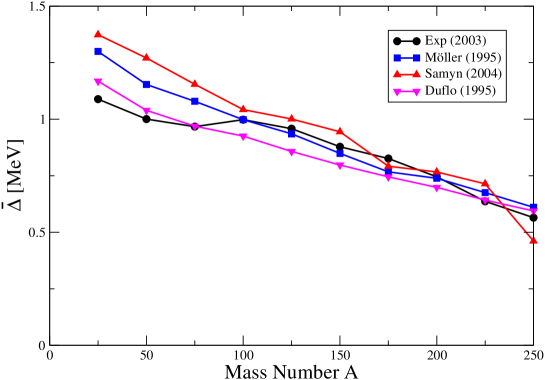
Figure 2: Average pairing gap versus mass number $A$ using the three-point measure, Eq. (1), with odd $M$. Binding energies are obtained from different theoretical mass models, Möller et al Moller (black dots), Samyn et al (red triangles pointing up) Samyn and Duflo et al (magenta triangles pointing down) Duflo . The theoretical curves are compared to experimental results (black dots), cf Fig.  1.

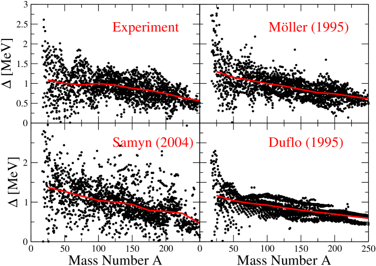
Figure 3: Pairing gaps extracted from Eq. (1) with odd $M$ versus mass number $A$ from experimental data, and three different theoretical mass models. Each black point corresponds to a nucleus. The solid red lines show the average pairing gap as shown in Fig. 2.

Figure 4: Root mean square (RMS) values of pairing gaps $\Delta$ obtained from Eq. (1) using odd $M$-values for three theoretical mass models, and experimental data. See caption of Fig. 2 for notations.

The pairing gap as defined by Eq. (1) can also be extracted from theoretical mass models, and in Fig. 2 we compare the average value of $\Delta_{3}$ versus particle number for three different mass models. Two of them are based on mean field theory. The first one is a non-self-consistent macroscopic-microscopic model Moller , the second one is a self-consistent calculation based on Skyrme-Hartree-Fock-Bogoliubov Samyn while the third one Duflo is a shell–model based calculation with parameterized monopole and multipole terms. Also the experimental mean value of the pairing gap is shown in Fig. 2, and it is seen that all three mass models give similar results in good agreement with experimental numbers. If, however, not average values, but pairing gaps obtained from all nuclei are shown (Fig. 3), it is clear that the average values give a poor description of the result. The fluctuations (RMS value) of the pairing gaps are indeed very large, and exhibit different variation with particle number for the different mass models, see Fig. 4. All mass formula show the same tendency of decreasing fluctuations with increasing mass number, as is also seen from experimental masses. However, considerably larger pairing fluctuations are seen in the mass model by Samyn et al Samyn , where, particularly for large mass numbers, almost three times larger fluctuations are obtained, as compared to pairing gap fluctuations obtained from measured masses. The mass model based on the shell–model Duflo gives systematically too small fluctuations, while the mass model by Möller et al Moller gives pairing fluctuations closest to experimental data.

It is thus clear that the fluctuations of the pairing gap is a most important property, and in the next section we shall present a semiclassical theory for pairing fluctuations based on periodic orbits Olofsson .

III Periodic orbit description of pairing fluctuations

The many-body Hamiltonian,

$$H=\hat{H}_{1}+\hat{V}_{\rm pair}=\sum_{k}e_{k}a^{\dagger}_{k}a_{k}-G\sum_{k\ell}a^{\dagger}_{k}a^{\dagger}_{\bar{k}}a_{\bar{\ell}}a_{\ell},$$ (4)

incorporates a one-body part, $\hat{H}_{1}$ (typically obtained from a deformed mean-field), and a two-body pairing interaction between time-reversed states, $\hat{V}_{\rm pair}$. All two-body matrix elements are assumed to take the same value, $G$ (seniority interaction). In the mean-field approximation in pairing space a pairing gap, or pairing ”deformation”,

$$\Delta=\left<G\sum_{k}a^{\dagger}_{k}a^{\dagger}_{\bar{k}}\right>,$$ (5)

is determined by the BCS gap equation BCS

$$\frac{2}{G}=\sum_{k}\frac{1}{\sqrt{(e_{k}-\lambda)^{2}-\Delta^{2}}},$$ (6)

that can be written as

$$\frac{2}{G}=\int_{-L}^{L}\frac{\rho(\varepsilon)d\varepsilon}{\sqrt{\varepsilon^{2}+\Delta^{2}}},$$ (7)

where $\rho(\varepsilon)$ is the single–particle level density, and we have put the Fermi energy, $\lambda$, to zero. The energy cut off is at $\pm L$.

Following semiclassical approaches, the pairing gap as well as the single-particle density of states are divided in a smooth part and a fluctuating part, $\Delta=\bar{\Delta}+\widetilde{\Delta}$ and $\rho=\bar{\rho}+\widetilde{\rho}$, respectively. In the weak coupling limit $\bar{\Delta}\ll L$, the smooth part of the gap is given by the well known solution $\bar{\Delta}=2L\exp(-1/\bar{\rho}G)$ (see e.g. Ref. BCS ). In semiclassical theory the fluctuating part of the density $\widetilde{\rho}$ can be calculated from purely classical properties semicl ,

$$\widetilde{\rho}(\varepsilon)=2\sum_{p}\sum_{r=1}^{\infty}A_{p,r}\cos(rS_{p}/\hbar+\nu_{p,r}),$$ (8)

where the sum is over all primitive periodic orbits $p$ (and their repetitions $r$) of the classical underlying effective single-particle Hamiltonian, $H_{1}$. Each orbit is characterized by its action $S_{p}$, stability amplitude $A_{p,r}$, period $\tau_{p}=\partial S_{p}/\partial\varepsilon$ and Maslov index $\nu_{p,r}$ (all evaluated at energy $\varepsilon$). Assuming $\widetilde{\Delta}\ll\bar{\Delta}$ and $\bar{\Delta}\ll L$ gives after some algebra Olofsson

$$\widetilde{\Delta}=2\frac{\bar{\Delta}}{\bar{\rho}}\sum_{p}\sum_{r=1}^{\infty}A_{p,r}K_{0}(r\tau_{p}/\tau_{\scriptscriptstyle\Delta})\cos\left(\frac{rS_{p}}{\hbar}+\nu_{p,r}\right),$$ (9)

where all classical quantities involved are evaluated at the Fermi energy. $K_{0}(x)$ is the modified Bessel function of second kind, and

$$\tau_{\scriptscriptstyle\Delta}=\frac{h}{2\pi\bar{\Delta}}$$ (10)

is a time corresponding to the pairing gap, that we may call the pairing time. Since $K_{0}(x)\propto\exp(-x)/\sqrt{x}$ for $x\gg 1$, the Bessel function exponentially suppresses all contributions for times $\tau\gg\tau_{\scriptscriptstyle\Delta}$ (making the sum in Eq. (9) convergent).

Since the value of the actions depend on the shape of the mean–field potential, Eq. (9) predicts generically fluctuations of the pairing gap as one varies, for instance, the particle number, or the shape of the system at fixed particle number. The fluctuations result from the interference between the different oscillatory terms that contribute to $\widetilde{\Delta}$. When the motion is regular (integrable), continuous families of periodic orbits having the same action, amplitude, etc, exist. The coherent contribution to the sum (9) of these families of periodic orbits produces large fluctuations. In contrast, in the absence of regularity or symmetries, incoherent contributions of smaller amplitude coming from isolated unstable orbits are expected for chaotic dynamics.

The second moment of the fluctuations may be obtained from Eq. (9) as Olofsson

$$\left<\widetilde{\Delta}^{2}\right>=2\frac{\bar{\Delta}^{2}}{\tau_{\scriptscriptstyle H}^{2}}\int_{0}^{\infty}d\tau K_{0}^{2}(\tau/\tau_{\scriptscriptstyle\Delta})K(\tau),$$ (11)

where $\tau_{\scriptscriptstyle H}=h/\delta$ is the Heisenberg time ($\delta=\bar{\rho}^{-1}$ is the single–particle mean level spacing at Fermi energy), and $K(\tau)$ is the spectral form factor, i.e. the Fourier transform of the two-point density–density correlation function Berry .

The structure of the form factor $K(\tau)$ is characterized by two different time scales. The first one, the smallest of the system, is the period $\tau_{\rm min}$ of the shortest periodic orbit. The form factor is zero for $\tau\leq\tau_{\rm min}$, and displays non-universal (system dependent) features at times $\tau_{\rm min}\stackrel{{\scriptstyle<}}{{\scriptstyle\sim}}\tau\ll\tau_{\scriptscriptstyle H}$. As $\tau$ further increases, the function becomes universal, depending only on the regular or chaotic nature of the dynamics, and finally tends to $\tau_{\scriptscriptstyle H}$ when $\tau\gg\tau_{\scriptscriptstyle H}$. The result of the integral (11) thus depends on the nature of the dynamics, and on the relative value of $\tau_{\scriptscriptstyle\Delta}$ with respect to $\tau_{\rm min}$ and $\tau_{\scriptscriptstyle H}$. In the simplest approximation, all the non–universal system–specific features are taken into account only through $\tau_{\rm min}$ Monastra , and one can write $K(\tau)=0$ for $\tau<\tau_{\rm min}$ and, for $\tau\geq\tau_{\rm min}$, $K(\tau)=\tau_{\scriptscriptstyle H}$ for integrable systems and $K(\tau)=2\tau$ for chaotic systems with time reversal symmetry. We assume a generic regular system; the analysis does not apply to the harmonic oscillator, whose form factor is pathological.

This finally gives the expressions for fluctuations of the pairing gap (normalized to the single–particle mean level spacing), $\sigma=\sqrt{\left<\widetilde{\Delta}^{2}\right>}/\delta$, assuming regular dynamics

$$\sigma_{\rm reg}^{2}=\frac{\pi}{4}\frac{\bar{\Delta}}{\delta}F_{0}\left(D\right)\ ,$$ (12)

and assuming chaotic dynamics,

$$\sigma_{\rm ch}^{2}=\frac{1}{2\pi^{2}}F_{1}\left(D\right)\ ,$$ (13)

where we have introduced the function Olofsson

$$F_{n}(D)=1-\frac{\int_{0}^{D}x^{n}K_{0}^{2}(x)dx}{\int_{0}^{\infty}x^{n}K_{0}^{2}(x)dx}.$$ (14)

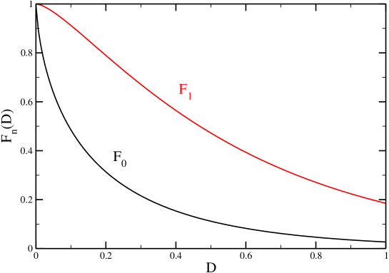
Figure 5: The two functions $F_{0}$ and $F_{1}$, see Eq. (14), versus the argument $D$.

The argument $D$ is defined as

$$D=\frac{\tau_{\rm min}}{\tau_{\scriptscriptstyle\Delta}}=\frac{2\pi}{g}\frac{\bar{\Delta}}{\delta},$$ (15)

where the parameter $g$ is the ratio between the Heisenberg time and the time of the shortest periodic orbit,

$$g=\frac{\tau_{H}}{\tau_{\rm min}}.$$ (16)

This parameter is often called ”dimensionless conductance”. It expresses the energy range, $L_{\rm max}(=g)$ (in dimensionless units; energies are divided by the mean energy spacing, $\delta$), in the single-particle spectrum where spectrum fluctuations show universal properties Berry . For a system where the corresponding classical dynamics is regular/chaotic (with time reversal symmetry), the statistical properties of the one-body energies, $e_{k}$ of Eq. (4) are described by Poisson/GOE (Gaussian Orthogonal Ensemble) statistics, respectively. The limit $g\rightarrow\infty$ (i.e. $D$=0), corresponds to a universal situation when the full spectrum corresponds to pure GOE (if chaotic) or Poisson (if regular) statistics.

The dimensionless parameter $D$ can also be expressed as the system size, $2R$, divided by the coherence length of the Cooper pair, $\xi_{0}=\hbar v_{\scriptscriptstyle F}/(2\bar{\Delta})$, where $v_{\scriptscriptstyle F}$ is Fermi velocity,

$$D=2R/\xi_{0}.$$ (17)

The Cooper pairs can thus be considered as restricted by the system size if $D<1$.

In Fig. 5 we show the two functions $F_{0}$ and $F_{1}$ of Eq. (14) versus the argument $D$. For small values of $D$, $F_{0}\approx 1$ and $F_{1}\approx 1$, and a universal behavior appears, i.e. the fluctuations do not depend on the system properties, only the dynamics, implying Poisson and GOE statistics for the full spectrum in the regular and chaotic cases, respectively. In the other limit when $D$ becomes large, $F_{0}$ and $F_{1}$ go to zero and all pairing fluctuations disappear. This is, for example, the situation in bulk systems with a large number of particles.

Figure 6: Fluctuations of the pairing gap as a function of the mean value for mesoscopic systems (log-log scale; all quantities normalized with the single-particle mean spacing). Regular and chaotic dynamics are shown by blue and red lines, respectively. The dashed curves correspond to different values of the dimensionless conductance, $g$, and the limiting case of $g\rightarrow\infty$ is shown by solid lines. The results are valid in the pairing regime $\bar{\Delta}/\delta>1$. Applications to Nuclei and Nano-grains are marked out. Ultracold atomic gases may be controlled to appear in major parts of the figure. From Ref. Olofsson .

In Fig. 6 pairing gap fluctuations are shown versus the pairing gap for different values of the dimensionless conductance, $g$, for regular as well as for chaotic dynamics. The plot covers a large range of parameter values and is shown in log-log scale. Pairing gaps of the order of the mean level spacing or smaller, $\bar{\Delta}<\delta$, (ultrasmall regime), are not treated by the present theory and corresponding region is shaded in the figure. In this region the Anderson condition Anderson implies no BCS pairing. As mentioned above, non-universal behavior (deviating from GOE or Poisson) appears when $D>0$, corresponding to finite values of the dimensionless conductance, $g$.

IV Fluctuations of pairing gap in nuclei

In a previous section we studied pairing gap fluctuations in nuclei as obtained from the odd-even mass difference, where binding energies were taken from different mass models as well as from data, see Fig. 4. We now would like to use the semiclassical theory developed in previous section to compare pairing gap fluctuations, and compare to these results. Notice that the theory does not contain any parameters. Once the system is defined, and the variable $D$ has been determined, the fluctuations only depend on the corresponding classical dynamics, being regular or chaotic. In nuclei ground states the dominating dynamics is expected to be regular, although elements from chaos may be present, see Ref.masses .

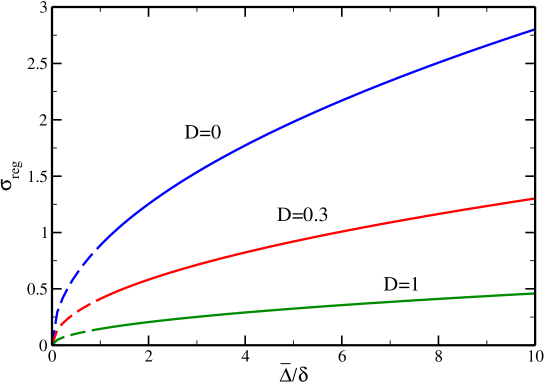
Figure 7: Fluctuations of pairing gap versus average pairing gap for different values of $D$. Regular dynamics is assumed. $D=0.3$ approximately corresponds to nuclei. Fluctuations and pairing gaps are expressed in units of the mean level spacing, $\delta$.

To evaluate the root mean square value (RMS) of the pairing fluctuations from the theoretical expressions, Eqs. (12) and (13), we only have to determine the parameter $D$. The size of the nucleus, $2R=2\times 1.2A^{-1/3}$ fm, and size of the pairing correlation length, $\xi_{0}=\hbar v_{F}/(2\bar{\Delta})=11.3A^{-1/4}$ fm, give (using Eqs. (2) and (17)) $D=2R/\xi_{0}=0.22A^{1/12}=0.27-0.33$ for mass numbers in the interval, $A$=25-250. The dependence of the pairing fluctuations, assuming regular dynamics, with the (average) pairing gap is shown in Fig. 7 for the three cases, $D$=0, 0.3 and 1. If the pairing correlation length is smaller than the system size ($D>1$) pairing fluctuations are quite small. Largest fluctuations appear in the universal limit when $D$=0. The small values of $D$ for nuclei ($D\approx$ 0.3) implies that the Cooper pairs are non-localized. The pairing gap fluctuations are thus substantial, and are about half the value at the universal limit.

Figure 8: RMS values of pairing gap fluctuations in nuclei versus mass number $A$, obtained from measured masses (dashed line connected by filled circles). Semiclassical calculations of the fluctuations assuming chaotic (Eq. (13)) and regular (Eq. (12)) dynamics are shown by red dashed and blue solid lines, respectively. From Ref. Olofsson

We may compare the fluctuations to the experimental pairing gap fluctuations by inserting the above values for $D$, and the average values of $\Delta$ from Eq. (2), in Eqs. (12) and (13), assuming regular or chaotic dynamics. The resulting curves are compared to the experimental one in Fig. 8. Note the good agreement between the theoretical pairing gap fluctuations assuming regular dynamics, and the experimental curve, both in the overall amplitude and in the $A$–dependence. In Ref.masses it was discussed the possibility that the dynamics of the nuclear ground state is mixed regular and chaotic. Making this assumption in the calculation of fluctuations of the pairing gap results in a curve that is very close to the purely regular curve in Fig. 8. That is, fluctuations of the pairing gap cannot distinguish if there is a chaotic component in the nuclear ground state.

V Shell structure in pairing gap from periodic orbit theory

Figure 9: A sample of classical periodic orbits of the cavity potential. The orbits shown correspond to the index $(v,w)$=(2,1), (3,1), (4,1), (5,2), (7,2) and (7,3), counted from upper left to lower right figure.

Figure 10: Nuclear pairing gaps for neutrons. Experimental isotope sequences are connected by thin solid lines. The blue dashed line shows average pairing gaps. Calculations from the cavity model are shown by the solid red line. Average behavior (Eq. (2)) is shown by solid black line. Data from Ref. NuclMass .

Shell effects in nuclei are also seen in the pairing gap. One may go beyond a statistical description, and use Eq. (9) to obtain a detailed description of the variation with neutron or proton numbers. For that purpose, we assume for the nuclear mean field a simple hard-wall cavity potential. The shape of the cavity at a given number of nucleons is fixed by minimization of the energy against quadrupole, octupole and hexadecapole deformations Hasse . To simplify, we take $N=Z$. The periodic orbits of the spherical cavity (a few short orbits are shown in Fig. 9) are used in Eq. (9), with modulations factors that take into account deformations and inelastic scattering creagh . This gives

$$\tilde{\Delta}=\frac{\bar{\Delta}}{\bar{\rho}E_{0}}\sum_{v,w}A_{vw}M_{vw}(x)\kappa_{\chi}(\ell_{vw})K_{0}\left(\frac{\ell_{vw}\bar{\Delta}}{2\bar{k_{F}}RE_{0}}\right)sin(\bar{k_{F}}R\ell_{vw}+\nu_{vw}\frac{\pi}{2}),$$ (18)

where $M_{vw}(x)$ is a modulation factor for perturbative deformations, $\kappa_{\chi}(\ell_{v\omega})$ a modulation factor for inelastic scattering, and $x$ stands for the three considered deformation degrees of freedom, quadrupole ($\varepsilon_{2}$), octupole ($\varepsilon_{3}$) and hexadecapole ($\varepsilon_{4}$). The summation is carried out over the two indices $(v,w)$ including the periodic orbits shown in Fig. 9. We set the average of $\widetilde{\Delta}$ to zero, as was done with the experimental data. In Fig. 10 we compare the theoretical result $\widetilde{\Delta}(N)$ to the experimental value averaged over the different isotopes at a given $N$. The agreement is excellent; the theory describes all the main features observed in the experimental curve.

VI Pairing fluctuations in nano-sized metallic grains

Experiments in the 90’s have explored the superconducting properties of nanometer scale aluminum grains RBT . Irregular shape of the grains implies chaotic dynamics, and energy levels are found to follow GOE (there are no further symmetries than time-reversal), see Ref. NanoRev . The existence of a superconducting gap was demonstrated in the regime $\bar{\Delta}>\delta$, whereas no gap was observed when $\bar{\Delta}<\delta$. The transition occurs around $N\sim 5000$, where $N$ is the number of conduction electrons in the grain. The $N$ dependence of the average gap $\bar{\Delta}$ is poorly understood. We will adopt for grains the thin-film value $\bar{\Delta}\approx 0.38\times 10^{-3}$ eV NanoRev . The mean level spacing is $\delta=(2E_{\scriptscriptstyle F})/(3N)\approx 2.1/N$ eV, whereas the dimensionless conductance, $g\approx 2.6N^{2/3}$. Eq. (15) gives $D\approx 4.4\times 10^{-4}N^{1/3}$, which ranges from $0.05$ to $0.02$ when $N$ varies between $10^{3}$ and $10^{5}$. This means that the variance will be close to its “universal” value (GOE limit) obtained by setting $F_{1}(D)=1$ in Eq. (13), namely Comm

$$\sigma^{2}_{\rm ch}=1/2\pi^{2}.$$ (19)

The typical range of variation of pairing gap fluctuations for nano-grains is marked out by a grey area in Fig. 6.

There are no explicitly measured pairing gap fluctuations for nanosized metallic grains to compare the present theory. We may, however, compare to other independent calculations, namely the condensation energy calculated of chaotic grains Dukelsky , and variation of the pairing gap with particle number in a regular cubic shaped grain Garcia .

The BCS condensation energy is defined as the total energy difference between the paired and the unpaired system. With our choice of gap equation (7) it is written as

$$E_{\rm C}=E_{\rm tot}(\Delta)-E_{\rm tot}(\Delta=0)=\int_{-L}^{L}\rho(e)ev^{2}(e)de-\frac{\Delta^{2}}{4G}-\int_{-L}^{0}\rho(e)edx$$ (20)

where $v^{2}(e)=\frac{1}{2}\left(1-\frac{e}{\sqrt{e^{2}+\Delta^{2}}}\right)$. Inserting the semiclassical approximations of $\rho=\bar{\rho}+\widetilde{\rho}$ and $\Delta=\bar{\Delta}+\widetilde{\Delta}$ and expanding $E_{\rm C}=\bar{E}_{\rm C}+\widetilde{E}_{\rm C}$ to lowest order in fluctuating properties, assuming $\widetilde{E}_{\rm C}\ll\bar{E}_{\rm C}$, gives

$$\widetilde{E}_{\rm C}=-2\sum_{p}\sum_{r=1}^{\infty}A_{p,r}\left[Q_{p,r}+qK_{0}(r\tau_{p}/\tau_{\scriptscriptstyle\Delta})\right]\cos\left(\frac{rS_{p}}{\hbar}+\nu_{p,r}\right)$$ (21)

where $K_{0}$ is the modified Bessel function of second kind, $q=\bar{\Delta}^{2}\left(1-\frac{1}{2\bar{\rho}G}\right)$ and

$$Q_{p,r}=\int_{-L}^{0}\cos\left(\frac{r\tau_{p}}{\hbar}\right)e\left(1+\frac{e}{\sqrt{e^{2}+\bar{\Delta}^{2}}}\right)de$$ (22)

The second moment, $\sigma_{\rm C}^{2}=\left<\widetilde{E}_{\rm C}^{2}\right>$, is thus obtained as

$$\sigma_{\rm C}^{2}=\frac{2}{h^{2}}\int_{0}^{\infty}\left[Q(\tau)+qK_{0}(\tau)\right]^{2}K(\tau)d\tau,$$ (23)

where $K(\tau)$ is the spectral form factor.

Figure 11: Fluctuations of the condensation energy as a function of the mean level spacing of the system. The blue solid and red dashed lines show the numerical calculations of regular and chaotic fluctuations according to Eq. (23). The squares show the calculations of ref. Dukelsky .

Using in addition the estimates $G=\frac{0.224}{\bar{\rho}}$ and $L=\frac{\bar{\Delta}}{2}e^{1/0.224}$ Dukelsky we show in Fig. 11 the fluctuations of the condensation energy, $\sigma_{\rm C}$, versus the level distance in the system, assuming regular and chaotic motion. As mentioned, there is no experimental data to compare to, but we may compare to a numerical calculation of the $\sigma_{\rm C}$ by Sierra et. al. Dukelsky where they use the Richardson’s solution of the pairing problem and random matrix theory (GOE) for generating the spectrum. We see that our semiclassical theory, assuming chaotic dynamics, agrees well with the random matrix calculation of Ref. Dukelsky . The random matrix model applied in Dukelsky happens to be a reasonable approximation for the considered nano-grains, since $D\approx 0$, i.e. the nano-grains have properties which are close to the universal limit.

Garcia-Garcia et al Garcia studied shell effects on the pairing gap in a cubic geometry as a function of the mean pairing gap, $\bar{\Delta}/\delta$. The cubic geometry implies classically regular motion, and we may thus use Eq. (12) above to calculate the fluctuation of the paring gap, normalized to the mean pairing gap $\bar{\Delta}$ instead of the mean level spacing $\delta$, $\sigma_{\rm reg}\delta/\bar{\Delta}=\sqrt{\frac{\pi}{4}\frac{\delta}{\bar{\Delta}}}$, where we have set $F_{0}=1$ since for small grains $D\approx 0$. This gives a very good agreement to the pairing fluctuations calculated in Ref. Garcia . It is interesting to note that by making the system chaotic, the pairing fluctuations decreases substantially and become (see Eq. (13)), $\sigma_{\rm ch}\delta/\bar{\Delta}=\frac{1}{\sqrt{2}\pi}\frac{\delta}{\bar{\Delta}}$, i.e. $\sigma_{\rm ch}/\sigma_{\rm reg}=\sqrt{\frac{2}{\pi^{3}}\frac{\delta}{\bar{\Delta}}}\approx 0.05$ if $\bar{\Delta}/\delta=20$.

VII Pairing fluctuations in ultracold fermionic gases

Recently, a large interest has emerged in studying trapped atomic gases of bosons and fermions. The gases are ultracold and dilute, and provide the possibility to study new quantum phenomena in the physics of finite many-body systems. The number of neutrons of the confined atoms determines the quantum statistics; odd number implies Fermions, and even number implies bosons. Studies of Bose condensates can be done for the bosonic gases, and studies of quantum phenomena including superfluidity and the transition to a Bose-Einstein condensate can be conducted for the Fermi gases.

Since the atom-atom interaction is short ranged and much smaller than the interparticle distance, the atom-atom interaction can be approximated by the $\delta$-interaction,

$$V(r_{1}-r_{2})=4\pi\frac{\hbar^{2}a}{m}\delta^{(3)}(r_{1}-r_{2}),$$ (24)

where $a$ is the s-wave scattering length, that can be externally controlled in size and even in sign through the Feshbach resonance. Also the confinement potential can be externally controlled to create regular as well as chaotic dynamics. Ultracold fermionic gases thus provide excellent conditions for theoretical as well as experimental studies of pairing properties, including pairing fluctuations. Since both particle number and interaction strength are experimentally controlled parameters, the fluctuations may appear in major parts of Fig. 6.

We estimate $\delta=(2E_{\scriptscriptstyle F})/(3N)$ and $g=\frac{1}{2}(3N)^{2/3}$; in the dilute BCS region $\bar{\Delta}=(2/e)^{7/3}E_{\scriptscriptstyle F}\exp\left(-\pi/2k_{\scriptscriptstyle F}|a|\right)$ Gorkov , with $k_{\scriptscriptstyle F}$ the Fermi wavevector, giving

$$D=\frac{2R}{\xi_{0}}=2\pi(2/e)^{7/3}(3N)^{1/3}\exp\left(-\pi/2k_{\scriptscriptstyle F}|a|\right).$$ (25)

Recent experiments using Li⁶ reach $k_{\scriptscriptstyle F}|a|=0.8$ KetterleLi6 , implying negligible fluctuations for typical values of $N\sim 10^{6}$. Reducing to $k_{\scriptscriptstyle F}|a|=0.2$ and $N=10^{4}$ yields for generic regular systems fluctuations that are on the same magnitude as the mean pairing gap, $\sigma_{\rm reg}\approx 0.5\bar{\Delta}/\delta$.

VIII Summary

In summary, we have presented a semiclassical theory that provides a generic description of fluctuations and shell structure of the BCS pairing gap in finite Fermi systems. These mesoscopic systems are generically dominated by system specific features not included in purely statistical models like GOE. Different possible regimes, as well as the influence of order/chaos dynamics, were investigated, in particular for the typical size of the fluctuations (Fig. 6). The present theory provides analytic predictions, valid for a wide range of physical situations. It also compares very favorably with available experimental data.

S.Å. thanks the Swedish Science Research Council, and P.L. acknowledges support by grants ANR–05–Nano–008–02, ANR–NT05–2–42103 and by the IFRAF Institute.

References

- (1) A. Bohr, B.R. Mottelson and D. Pines, Phys. Rev. 110, 936 (1958).
- (2) H. Olofsson, S. Åberg, P. Leboeuf, Phys. Rev. Lett. 100, 037005 (2008).
- (3) J. Dobaczewski et al., Phys. Rev. C 63, 024308 (2001).
- (4) G. Audi, A.H. Wapstra and C. Thibault, Nucl. Phys. A729, 337 (2003).
- (5) P. Möller, J. R. Nix, W. D. Myers, and W. J. Swiatecki, At. Data and Nucl. Data Tables 59 (1995) 185.
- (6) M. Samyn, S. Goriely, M. Bender, and J. M. Pearson, Phys. Rev. C 70, 044309 (2004).
- (7) J. Duflo and A. P. Zuker, Phys. Rev. C 52, R23 (1995).
- (8) D. Brink and R.A. Broglia, Nuclear Superfluidity: Pairing in Finite Systems (Cambridge Univ. Press, 2005).
- (9) M. Brack and R.K. Bhaduri, Semiclassical Physics (Addison and Wesley, Reading, 1997).
- (10) M.V. Berry, Proc. Roy. Soc. Lond. A 400, 229 (1985).
- (11) P. Leboeuf and A.G. Monastra, Ann. Phys. 297, 127 (2002).
- (12) P.W. Anderson, J. Phys. Chem. Solids B 11, 26 (1959).
- (13) O. Bohigas and P. Leboeuf, Phys. Rev. Lett. 88, 092502 (2002).
- (14) R. Hasse, Ann. Phys. 68, 377 (1971).
- (15) S. C. Creagh, Ann. Phys. (N.Y.) 248, 60 (1996); P. Leboeuf, Lect. Notes Phys. 652, Springer, Berlin Heidelberg 2005, p.245, J. M. Arias and M. Lozano (Eds.).
- (16) D.C. Ralph, C.T. Black and M. Tinkham, Phys. Rev. Lett. 74, 3241 (1995); ibid 76, 688 (1996)
- (17) J. von Delft and D.C. Ralph, Phys. Rep. 345, 61 (2001).
- (18) The expression for pairing fluctuations in the universal GOE limit (corresponding to =0) was first derived in ML .
- (19) K.A. Matveev and A.I. Larkin, Phys. Rev. Lett. 78, 3749 (1997).
- (20) G. Sierra et al., Phys. Rev. B 61, 11890 (2000).
- (21) M. Garcia-Garcia et al, arXiv:0710.2286 (2007).
- (22) L.P. Gor’kov and T.K. Melik-Barkhudarov, Sov. Phys. JETP 13, 1018 (1961).
- (23) C.H. Schunck et al., Phys. Rev. Lett. 98, 050404 (2007).