Implications of multi-Regge limits for the Bern-Dixon-Smirnov conjecture

Abstract

Planar ${\cal N}=4$ super Yang-Mills $SU(N)$ theory is expected to exhibit stringy behavior, anticipated by the ’t Hooft genus expansion and the $AdS/CFT$ correspondence. We examine the Bern-Dixon-Smirnov (BDS) conjecture for $n$-gluon amplitudes in the context of single-Regge and multi-Regge limits and show that these amplitudes have the expected Regge form in the Euclidean region.

1 Introduction

The $AdS/CFT$ correspondence, in conjunction with recent work, has made it possible to study $n$-gluon scattering amplitudes in the $SU(N)$ planar ${\cal N}=4$ super Yang-Mills (SYM) theory, both at weak and strong coupling. In this context Bern, Dixon and Smirnov (BDS) [1] (see also [2]) have made a conjecture for the color-ordered maximal helicity-violating (MHV) $n$-gluon amplitudes. Further, Alday and Maldacena (AM) presented a strong-coupling description of the $n$-gluon amplitude using the $AdS/CFT$ correspondence [3]. Schematically their solution is of the form

$${\cal A}_{n}=A_{tree}e^{\textstyle-\frac{\sqrt{\lambda}}{2\pi}A_{min}(C_{n})}$$ (1.1)

where $A_{min}(C_{n})$ is the minimal area for a surface in $AdS_{5}$ spanning the contour $C_{n}$ made of $n$ light-like segments with the $i$th side given by the on-shell gluon momentum $k^{\mu}_{i}$. Alday and Maldacena pointed out that after regularization, the finite part of (1.1) for $n=4$ agrees with the BDS conjecture. Motivated by this, it was conjectured that there exists a duality between the gluon amplitudes and light-like Wilson loops also at weak-coupling, and proven at 1 loop in [4, 5]. This duality has been verified at two-loops for $n=4$ and $n=5$, and a conformal Ward identity was derived for the light-like Wilson loops $W(C_{n})$, presumed to be valid to all orders in the ’t Hooft coupling, $\lambda=g^{2}N$[6, 7]. The Ward identity fixes the finite part of the Wilson loop for $n=4$ and $n=5$, up to an additive constant, and agrees with the BDS conjecture for these amplitudes. Recently doubt has been cast on the BDS conjecture for $n\geq 6$. In particular AM [8] argued that for a large number of gluons the Wilson loop disagrees with the BDS conjecture, although their results might still be compatible with a possible duality between the gluon amplitudes and the Wilson loops. There has also been explicit consideration of the $n=6$ amplitude, where problems with the BDS conjecture are encountered. Astefanesei et. al. [9] analyze the strong-coupling prediction of the BDS conjecture for $n=6$ and find discrepancies with the $AdS/CFT$ prescription of AM. The finite part of the BDS $n=6$ amplitude was also compared to the hexagonal light-like Wilson loop at two loops [10], with the two expressions differing by a non-trivial function of the three (dual) conformal invariant variables.

Since large N $SU(N)$ ${\cal N}=4$ SYM is closely related to a string theory by means of the $AdS/CFT$ correspondence, it is reasonable to expect that ${\cal N}=4$ SYM theory exhibits evidence of stringy behavior. Further this is already anticipated by ’t Hooft’s large N expansion of the theory as a genus expansion. In flat-space string theory, it is well-known that scattering amplitudes exhibit Regge behavior at high energy with fixed momentum transfer, $t$, e.g., for 2-to-2 scattering,

$$A(s,t)\sim\beta(t)(s/t)^{\alpha(t)}$$ (1.2)

where $\alpha(t)$ is the Regge trajectory function, see Fig. 1. Indeed the $n=4$ BDS gluon amplitude can be recast [4, 11] so as to exhibit Regge behavior, with a Regge trajectory for the gluon and Regge residue given to all orders in perturbation theory in terms of the cusp anomalous dimension [12, 13]. Given the AM results, strong-coupling limits of the trajectory function and residue are included as well.

Given the view that ${\cal N}=4$ SYM has string behavior and the Regge behavior of the $n=4$ gluon amplitude, it is suggestive that the gluon scattering amplitudes for $n\geq 5$ might also be expected to exhibit Regge and multi-Regge behavior. It is the objective of this paper to examine this issue for $n\geq 5$ BDS gluon amplitudes. We find that the BDS amplitudes have the expected Regge and multi-Regge behavior in various Euclidean limits. A crucial tool in establishing this result is an understanding of the cross-ratios in various Regge limits. This may have significance beyond ${\cal N}=4$ SYM.

Further, we relate the solution to the conformal Ward identity for the lightlike polygon Wilson loop proposed in [6, 7] to the Regge behavior of the BDS amplitude, giving support to the strong coupling Wilson loop/gluon amplitude duality implied by the Alday-Maldacena proposal. (Note that this duality fails at finite temperature [14]).

In Sec. 2 we review the BDS conjecture and the Regge behavior of the $n=4$ amplitude. In Sec. 3 we describe the Regge and multi-Regge limits of general $n>4$ amplitudes. In Sec. 4, we successfully recast the $n=5$ BDS amplitude to reveal its Regge behavior. In Sec. 5 we consider the Regge and multi-Regge limits of the $n=6$ BDS amplitude. Sec. 6 extends the discussion to the BDS amplitudes for $n\geq 7$. In Sec. 7 we relate the Wilson loop solution to the conformal Ward identity to the Regge behavior of the BDS amplitudes. In Sec. 8 we summarize our results. Appendix A describes details of the BDS variables and constraints, while Appendix B contains details omitted from Sec.  6.

2 The four-gluon amplitude

The Reggeization of the gluon in non-supersymmetric Yang Mills theories [15, 16, 17, 18, 19], as well as supersymmetric Yang Mills  [20, 21, 22, 23], has a long history. We review this issue for ${\cal N}=4$ SYM in the context of the BDS conjecture for the on shell 2-2 gluon scattering amplitude, ${\cal A}_{4}(k_{1}+k_{2}\rightarrow-k_{3}-k_{4})$, where the Mandelstam variables are $s=(k_{1}+k_{2})^{2}$, $t=(k_{1}+k_{4})^{2}$ and $u=(k_{1}+k_{3})^{2}$, with $s+t+u=0$. The $1-2-3-4$ color ordered four point amplitude in the BDS conjecture is

$${\cal A}_{4}={A}_{tree}{A}^{2}_{div}(s){A}^{2}_{div}(t)\;e^{\textstyle\textstyle\frac{f(\lambda)}{8}\log^{2}(s/t)+\widetilde{c}(\lambda)}$$ (2.1)

where $f(\lambda)$ is proportional to the cusp anomalous dimension and in $d=4-2\epsilon$ the IR divergent contribution is

$${A}_{div}(s)=\exp\left[-\frac{1}{8\epsilon^{2}}f^{(-2)}\left(\lambda(\frac{\mu^{2}}{-s})^{\epsilon}\right)-\frac{1}{4\epsilon}g^{(-1)}\left(\lambda(\frac{\mu^{2}}{-s})^{\epsilon}\right)\right]$$ (2.2)

where $\lambda=g^{2}N$, and $\mu$ is a scale introduced with the IR regulator. Expanding in $\epsilon$, one obtains $f(\lambda)$ and $g(\lambda)$ [1, 3, 12, 13, 24, 25, 26, 27]

$$f(\lambda) = (\lambda\frac{d}{d\lambda})^{2}f^{(-2)}(\lambda)=(\lambda\frac{d}{d\lambda})f^{(-1)}(\lambda)$$ (2.3)

$$g(\lambda) = (\lambda\frac{d}{d\lambda})g^{(-1)}(\lambda)$$

where $\widetilde{c}(\lambda)$ is a a constant. In weak coupling,

$$f(\lambda) = \frac{\lambda}{2\pi^{2}}+O(\lambda^{2})$$

$$g(\lambda) = O(\lambda^{2})$$ (2.4)

$$\widetilde{c}(\lambda) = \frac{\lambda}{16\pi^{2}}(\frac{4\pi^{2}}{3})+O(\lambda^{2})$$

Although ${\cal A}_{4}(s,t)$ is manifestly symmetric in $s\leftrightarrow t$, with ${\cal A}_{tree}\sim(s/t)$ for $|s/t|>>1$, a straight forward calculation gives

$${\cal A}_{4}(s,t)=\beta(t)(s/t)^{\alpha(t)}$$ (2.5)

where the gluon trajectory function  is

$$\alpha(t)=1+\frac{1}{4\epsilon}f^{(-1)}(\lambda)-\frac{1}{4}f(\lambda)\log(-t/\mu^{2})+{\frac{1}{2}}g(\lambda)$$ (2.6)

Figure 1: Regge amplitude for elastic 4-point amplitude defines and fixes the trajectory function $\alpha(t)$ and the Reggeon vertex, $\gamma(t)$.

and the Regge residue is

$$\beta(t)\equiv\gamma^{2}(t)=\;\mbox{const}\;[{A}_{div}(t)]^{4}\;e^{\textstyle\widetilde{c}(\lambda)}\;,$$ (2.7)

as in Fig.1, where the Sudakov factor

$$A_{div}(t)=\exp\left\{-\frac{1}{16}f\left(\lambda\right)\log^{2}(-t/\mu^{2})+\left[\frac{1}{8\epsilon}f^{(-1)}\left(\lambda\right)+\frac{1}{4}g\left(\lambda\right)\right]\log(-t/\mu^{2})\right\}$$ (2.8)

contains in the exponent a term quadratic in $\log(-t/\mu^{2})$ and the $O(1/\epsilon^{2})$ divergent constant has been dropped. One way to see how to go from (2.1) to (2.5) is to recognize that

$${A}_{div}(s) = {A}_{div}(t)$$ (2.9)

$$\times \exp[+\frac{1}{8\epsilon}f^{(-1)}(\lambda)\log(s/t)+\frac{1}{4}g(\lambda)\log(s/t)$$

$$- \frac{1}{16}f(\lambda)\log^{2}(-s/\mu^{2})+\frac{1}{16}f(\lambda)\log^{2}(-t/\mu^{2})]\;,$$

It is crucial to note the cancellation of the $\log^{2}(s/t)$ in Eq. (2.1) with the $\log^{2}(-s/\mu^{2})$ in ${\cal A}_{div}$ in leading to the Regge amplitude (2.5). We also note that Eq. (2.5) is first defined in the Euclidean region where $s,t<0$ and then continued to the physical region where $s>0$ and $t<0$, with the phase of the amplitude given by $(s/t)^{\alpha}=e^{-i\pi\alpha}(s/-t)^{\alpha}$. In our subsequent multi-Regge analysis we will not spell out explicitly phases resulting from continuation to the physical scattering region. The important issue of phase in the multi-Regge limit will be consider in subsequent work.

Note that the trajectory (2.6) goes as $-\log(-t/\mu^{2})$ rather than rising linearly with $t$, suggesting stringy behavior, but in the infinite tension limit. There are no Regge recurrences and no scale for the slope $\alpha^{\prime}$, consistent with a ${\cal N}=4$ conformal theory with no massive states. 

3 Regge limits of $n>4$ amplitudes

For $n>4$ amplitudes, the Regge limits are more complicated. In particular, one has to distinguish between single-Regge limits, that are a direct generalization of the Regge limit of the 4-point amplitude, where a single momentum invariant quantity (the analog of $s$ for 4-point) goes to infinity, and multi-Regge limits, where several momentum invariant quantities go to infinity ($s_{1},...,s_{k}$). Moreover, there are large class of multi-Regge limits. Here we will restrict ourselves to the single-Regge and the extreme multi-Regge example, the so-called “linear multi-Regge” limit, since they are diagrammatically easy to understand and will be used in the general n-point analysis in Sec. 6. For more details on multi-Regge limits and their realization in flat space open string theory, see the review [28].

It should be emphasized that the Regge hypothesis, although based on a long history of experience, is not a proven property in detail, particularly for a conformal field theory, let alone for ${\cal N}=4$ SUSY. However as one gains confidence in the Regge properties, they do become an increasingly plausible and powerful non-perturbative constraint. Indeed this was one of the salient constraints originally used in the discovery of flat-space string theory. To be specific consider the single-Regge limit for a 2-to-(n-2) amplitude as illustrated in Fig 3. The large invariant is taken to be $s_{m}=(k_{m+1}+k_{m+2})^{2}$ with rapidity gap $y\sim\log(s_{m})\rightarrow\infty$. Without loss of generality, we consider the group of particles with momenta $k_{1},\cdots,k_{m+1}$ to be “right movers” with large postive velocities on the z-axis and particles with $k_{m+2},\cdots,k_{n}$ to be “left movers” with large negative velocities on the z-axis . In light-cone coordinates, the right and left movers have large components $k^{+}=(k^{0}+k^{3})/\sqrt{2}$ and $k^{-}=(k^{0}-k^{3})/\sqrt{2}$ respectively so the Regge limit can be identified with a matrix element of a Lorentz boost,

$${\cal A}_{n}(s)\simeq\langle\bar{k}_{1},\cdots,\bar{k}_{m+1}|\;\exp[yM_{+-}]\;|\bar{k}_{m+2},\cdots\bar{k}_{n}\rangle\;$$ (3.1)

The matrix element is taken between states boosted to a frame with (near) zero z-momenta so that the relative boost back to the original frame is given by the rapidity difference, $y=y_{R}-y_{L}\sim\log(s_{m})$. A detailed analysis  [29, 30, 31] leads to the consequence that the singularities in the angular-momentum $J$-plane are determined by the spectrum of the boost operator, $M_{+-}$, through the Mellin-Laplace transform,

$${\cal A}_{n}(j)\simeq\int^{\infty}_{\mu^{2}}ds\;s^{-j-1}\;{\cal A}(s)\quad\sim\quad\langle\bar{k}_{1},\cdots,\bar{k}_{m+1}|\frac{1}{j-M_{+-}}|\bar{k}_{m+2},\cdots,\bar{k}_{n}\rangle\;.$$ (3.2)

If the largest eigenvalue eigenvalue for $M_{+-}$ is discrete, there is a leading simple pole in the $J$-plane and a dominant pure power $s_{m}^{\alpha(t_{m})}$ for the amplitude at high energies. A fundamental hypothesis of Regge theory states that all amplitudes with the same quantum numbers must share exactly the same $J$-plane poles and the residues factorize .

Remarkably the exact 4-point BDS amplitude has been found to corresponds to a single $J$-plane pole plus integer space daughters [4, 11]. This property of an exact meromorphic $J$-plane also holds for the BDS 5-point function. The similarity between the BDS $J$-plane and flat space string theory is striking. The classic 4-point Veneziano amplitude of flat space string theory is also meromorphic in the $J$-plane with integer spaced daughters. Since flat space string theory is integrable, it is known that there is the absense of Regge cuts in the planar limit, which raises the question of whether planar ${\cal N}=4$ SYM might also exhibit pure $J$-plane meromorphy with simple poles and no Regge cuts.

Figure 2: n-point amplitude expressed as a tree diagram of effective particle (”Reggeon”) exchange in order to emphasize the parameterization of the linear multi-Regge limit.

The focus of this article is restricted to the examination of the leading Regge and multi-Regge behavior for the conjetured BDS amplitudes for $n>4$ in the Euclidean region. The BDS ansatz for a general $n$-point is conveniently expressed in terms of an over complete set of cyclic “Mandelstam” invariants $t_{i}^{[r]}\equiv(k_{i}+...+k_{i+r-1})^{2}$ for all unitarity cuts of the n-point function with the external legs arranged in the cyclic order of the large N single color trace. There are $n(n-3)/2$ such distinct cyclic invariants, but due to $n$ mass-shell conditions and 10 Lorentz symmetries, this reduces the $4n$ momentum components, $k^{\mu}_{i}$ to $3n-10$ independent Lorentz variables. Hence there are constraints for $n\geq 6$. Fortunately in the Regge limit the constraints take a simple form. (see Appendix A for more details on these constraints.)

First let us consider an independent set of invariants most appropriate for the 2-to-(n-2) amplitude in the linear multi-Regge limit. Here one views the $n$-point amplitudes as tree level interactions involving effective particle (”Reggeon”) exchange, as in Fig. 2. Associated with this configuration, it is natural to define $n-3$ two body energy invariants, $s_{i}$, and $n-3$ momentum transfers, $t_{i}$.

$$s_{i}=t_{i+1}^{[2]}\;,\quad i=1,...,n-3\;,\quad{\rm and}\quad t_{r}=t_{1}^{[r+1]}\;,\;\quad r=1,...,n-3\;.$$ (3.3)

Clearly $\{s_{i}\}$ and $\{t_{r}\}$ may be regarded as generalization of $s$ and $t$ for the 4-point amplitude. In the linear multi-Regge limit, all $\{s_{i}\}$ goes to infinity with $\{t_{r}\}$ fixed. For the remaining $n-4$ independent variables, we provisionally choose the three body energies,

$$\Sigma_{i}=t_{i+1}^{[3]},\;\quad i=1,...,n-4\;.$$ (3.4)

An alternative choice, which is more convenient for discussing various Regge limits, is to scale $\Sigma_{i}$ by defining ratio variables

$$\kappa_{i}\equiv\frac{\Sigma_{i}}{s_{i}s_{i+1}},\;\quad i=1,...,n-4$$ (3.5)

An n-point amplitude can be considered as a function of this set of $3n-10$ independent variables, ${\cal A}_{n}(s_{1},\cdots,s_{n-3},t_{1},\cdots,t_{n-3},\kappa_{1},\cdots,\kappa_{n-4})\;$. All other BDS invariants can be expressed in terms of this set (see Appendix A.)

Single Regge Limit: In this limit there is a single large rapidity gap, which for the general n-point function we take to be given by $\log(s_{k})\sim\log(s)\rightarrow\infty$, which cuts the diagram into two halves of right and left movers as described before and illustrated in Figs. 2 and 3. This implies a Reggeon propagator carrying an invariant mass squared $t_{k}$ dual to the cut,

$${\cal A}_{n}\sim s_{k}^{\alpha(t_{k})}$$ (3.6)

A nice pictorial way to represent the single Regge limit it is to draw a dotted line cutting through the corresponding “Reggeon exchange” line, in our example dotted line $k$ cutting through $t_{k}$ and separating particles $1$ through $k+1$ from the rest, Fig. 2. Then any of the BDS invariants, $[i,i+r]$, that contains momenta on both sides of the dotted line, (expressed either as $t_{i}^{[r]}$ or as $t_{i+r}^{[n-r]}$, i.e., $[i,i+r]\;({\rm mod}\;n)=t_{i}^{[r]}=t_{i+r}^{[n-r]}$), will go to infinity. Thus in this example, from the set of independent variables $\{s_{i},t_{j},\Sigma_{i}\}$, only $s_{k}$ and $\Sigma_{k-1},\Sigma_{k}$ go to infinity (if $k\neq 1$), and all the others stay fixed. Furthermore, since $s_{k}\sim\Sigma_{k-1}\sim\Sigma_{k}$, it follows that $\kappa_{k}$ is fixed. That is, this single-Regge limit is defined by $s_{k}\rightarrow\infty$, with $s_{1},s_{2}\cdots,s_{n-3},\;(\neq s_{k}),t_{1},t_{2},\cdots,t_{n-3}$, and $\kappa_{1},\kappa_{2},\cdots,\kappa_{n-4}$ fixed.

As the number of external lines is increased this leads to a sequence of single-Regge limits,

$${\cal A}_{4} \simeq [\gamma(t)]^{2}\left(\frac{s}{t}\right)^{\alpha(t)}$$ (3.7)

$${\cal A}_{5} \simeq \gamma(t_{1})\left(\frac{s_{1}}{t_{1}}\right)^{\alpha(t_{1})}G^{[3]}_{1}(t_{1},s_{2},\kappa_{1},t_{2})$$ (3.8)

$${\cal A}_{6} \simeq \gamma(t_{1})\left(\frac{s_{1}}{t_{1}}\right)^{\alpha(t_{1})}G^{[4]}_{1}(t_{1},\kappa_{1},s_{2},t_{2},\kappa_{2},s_{3},t_{3})$$ (3.9)

$${\cal A}_{6} \simeq G^{[3]}_{1}(t_{1},s_{1},\kappa_{1},t_{2})\left(\frac{s_{2}}{t_{2}}\right)^{\alpha(t_{2})}G^{[3]}_{1}(t_{2},s_{3},\kappa_{2},t_{3})$$ (3.10)

$${\cal A}_{7} \simeq \cdots\cdots$$

all of which must share the same Regge trajectory function, $\alpha(t)$ and the “residues” for different amplitudes factorize into a single sequence of Reggeon k-particle vertex functions: $\gamma(t)$, $G_{1}^{[k]}(t_{i},s_{i},\kappa)$. This places a strong recursive consistency condition on the BDS construction. In essence this condition reflects the existence of a well defined spectral decomposition for the boost operator $M_{+-}$ analogous to the spectral condition for a Hamiltonian. In particular once $\gamma(t)$ is determined from ${\cal A}_{4}$ and $G^{[3]}_{1}$ from ${\cal A}_{5}$, the symmetric Regge (3.10) limit of ${\cal A}_{6}$ is entirely fixed. We show that the BDS conjecture satisfies these constraints.

As we will see in our subsequent analysis the crucial simplification of the BDS amplitude in the Regge limits relates to the limit of conformal cross-ratios . The way this works is as follows. The n-point function has momenta $k_{i}$ with one energy-momentum constraint, $k_{1}+k_{2}+\cdots+k_{n}=0$. This constraint is satisfied by introducing $n$ variables $x_{i}$ on the dual vertices of the dual polygon with $k_{i}$ assigned to the edges such that $k_{i}=x_{i}-x_{i+1}$ and the variables

$$x_{i,j}=x_{i}-x_{j}=k_{i}+\cdots+k_{j-1}$$ (3.11)

so that the BDS variables are redefined as unique differences,

$$t^{[r]}_{i}=t^{[n-r]}_{i+r}=x^{2}_{i,i+r}\equiv(x_{i}-x_{i+r})^{2}$$ (3.12)

In computation, the notation $[i,j]\equiv x^{2}_{i,j}$ often proves to be convenient. All indices are treated cyclically modular $n$. The BDS amplitudes make special use of conformally invariant cross ratios,

$$u(i,j;a,b)=\frac{x^{2}_{i,j}x^{2}_{a,b}}{x^{2}_{i,b}x^{2}_{a,j}}=\frac{[i,j][a,b]}{[i,b][a,j]}\;.$$ (3.13)

As an example in single-Regge limits consider a cross ratio where all 4 invariant factors connect the right movers ($k^{+}_{R}\rightarrow\infty$ for $R=2,\cdots,k+1$) with the left movers ($k^{-}_{L}\rightarrow\infty$ for $L=k+2,\cdots,n-1$) as depicted in Fig. 3.

Figure 3: Cross ratios in the single-Regge limit

The $s_{k}\rightarrow\infty$ limit implies that all such cross ratios,

$$u(i,j,p,q)=\frac{x_{i,j}^{2}x_{p,q}^{2}}{x_{i,q}^{2}x_{p,j}^{2}}=\frac{(k_{i}+...+k_{j-1})^{2}(k_{p}+...+k_{q-1})^{2}}{(k_{i}+...+k_{q-1})^{2}(k_{p}+...+k_{j-1})^{2}}\rightarrow 1+O(1/s_{k})$$ (3.14)

approach 1. This follows immediately from the fact that scalar products ($p_{R}q_{L}\simeq p^{+}_{R}q^{-}_{L})$ between right and left movers become large,

$$u(i,j,p,q)\simeq\frac{(P^{+}Q^{-})(p^{+}q^{-})}{(P^{+}q^{-})(p^{+}Q^{-})}=1\;,$$ (3.15)

where we have collected the partial sums into $P^{\mu}=\sum_{R=i}^{k+1}k_{R}^{\mu}$, $p^{\mu}=\sum_{R=p}^{k+1}k_{R}^{\mu}$ and $Q^{\mu}=\sum_{L=k+2}^{j-1}k_{L}^{\mu}$, $q^{\mu}=\sum_{L=k+2}^{q-1}k_{L}^{\mu}$. This is a crucial kinematic feature leading to Regge behavior for the BDS ansatz. Other specific examples of the simplification of the constraints in the Regge limit are given in the following text as we need them and summarized in Appendix A.

Linear Multi-Regge Limit: Interpreting the Regge limit in terms of large rapidity separation allows a systematic generalization to multi-Regge limits  [32, 33]. The basic idea is to consider the external momenta ordered by rapidities and to separate them in groups with infinite rapidity differences between them.

The “linear multi-Regge” limit (also known as “multi-peripheral limit”) is defined by taking several infinite rapidity gaps, corresponding to several of the dotted lines in Fig. 2. The maximal case is when all $n-3$ lines correspond to infinite rapidity gaps. Then all of the $s_{i}$ go to infinity independently, i.e., the limit is defined by $s_{1},s_{2},\cdots,s_{n-3}\rightarrow\infty$ holding $t_{1},t_{2},\cdots,t_{n-3},\kappa_{1},\kappa_{2},\cdots,\kappa_{n-4}$ fixed. In this limit, since $s$ is linear in each $s_{i}$, it can be shown that

$$s\simeq\;b_{0}s_{1}s_{2}\cdots s_{n-3}\;.$$ (3.16)

where $b_{0}=\Pi_{i=1}^{n-4}\kappa_{i}$. The postulated behavior for this “maximal multi-Regge limit” is

$${\cal A}_{5} \simeq \gamma(t_{1})\left(\frac{s_{1}}{t_{1}}\right)^{\alpha(t_{1})}G_{2}(t_{1},\kappa_{1},t_{2})\left(\frac{s_{2}}{t_{2}}\right)^{\alpha(t_{2})}\gamma(t_{2})$$ (3.17)

$${\cal A}_{6} \simeq \gamma(t_{1})\left(\frac{s_{1}}{t_{1}}\right)^{\alpha(t_{1})}G_{2}(t_{1},\kappa_{1},t_{2})\left(\frac{s_{2}}{t_{2}}\right)^{\alpha(t_{2})}G_{2}(t_{2},\kappa_{2},t_{3})\left(\frac{s_{3}}{t_{3}}\right)^{\alpha(t_{3})}\gamma(t_{3})$$

$$\cdots\cdots$$

$${\cal A}_{n} \simeq \gamma(t_{1})\left(\frac{s_{1}}{t_{1}}\right)^{\alpha(t_{1})}G_{2}(t_{1},\kappa_{1},t_{2})\cdots\cdots\left(\frac{s_{n-3}}{t_{n-3}}\right)^{\alpha(t_{n-3})}\gamma(t_{n-3})$$ (3.19)

In this limit, kinematic simplifications can be achieved since, for $2\leq i<j\leq n$,

$$[i,j]=x_{i,j}^{2}=t_{i}^{[j-i]}=(\sum_{r=i}^{j-1}k_{r})^{2}\simeq 2k^{+}_{i}\cdot k^{-}_{j-1}+0(1)\;.$$ (3.20)

Moreover, $\kappa_{i}$ now has a simple physical interpretation,

$$\kappa_{i-2}\simeq(2k^{+}_{i}k^{-}_{i})^{-1}={k_{i,\perp}^{2}}^{-1}$$ (3.21)

so that the sub-energy invariant $s_{i}$ is proportional to the ratio $k^{+}_{i+1}/k^{+}_{i+2}$,

$$s_{i}\simeq 2k^{+}_{i+1}k^{-}_{i+2}\simeq{k_{i+2,\perp}^{2}}(k_{i+1}^{+}/k_{i+2}^{+})>>1\;.$$ (3.22)

For more details on these kinematic constraints see Appendix A.

4 The BDS five-gluon amplitude

The BDS conjectured $n=5$ amplitude for the on shell gluon amplitude with $k_{1}+k_{2}+k_{3}+k_{4}+k_{5}=0$ and $t^{[r]}_{i}=(k_{i}+\cdots+k_{i+r-1})^{2}$ is given by

$${\cal A}={A}_{tree}\prod^{5}_{i=1}A_{div}(t^{[2]}_{i})e^{\textstyle{\cal F}_{5}(0)}$$ (4.1)

where

$${\cal F}_{5}(0) = \frac{f(\lambda)}{8}(L_{5}+\frac{15}{2}\zeta_{2})\;,\quad$$ (4.2)

and

$$L_{5}=-{\frac{1}{2}}\sum_{i=1}^{5}\log(\frac{-t^{[2]}_{i}}{-t^{[2]}_{i+3}})\log(\frac{-t^{[2]}_{i+1}}{-t^{[2]}_{i+2}})$$ (4.3)

Let us choose a specific kinematical configuration for definiteness, appropriate to $1+5\rightarrow\bar{2}+\bar{3}+\bar{4}$, as in Fig  4.

Figure 4: Regge limits for 5-point amplitude. On the left, the single Regge limit factorizes defining a new single Regge 3-particle vertex, $G^{[3]}(t_{1},\kappa_{12},s_{2},t_{2})$ and on the right, the double Regge limit defines a new two-Reggeon vertex, $G_{2}(t_{1},\kappa_{1},t_{2})$.

The variables correspond to the BDS variables as follows,

$$t^{[2]}_{1}=t_{1};\;\;t^{[2]}_{2}=s_{1};\;\;t^{[2]}_{3}=s_{2};\;\;t^{[2]}_{4}=t_{2};\;\;t^{[2]}_{5}=\Sigma_{1}=s$$ (4.4)

As discussed in sec. 3, we will use, instead of $\Sigma_{1}$, an alternative ratio variable

$$\kappa_{1}=\frac{\Sigma_{1}}{s_{1}s_{2}}=\frac{s}{s_{1}s_{2}}$$ (4.5)

Thus using relations (2.9) in (4.1) it is a straightforward algebraic exercise to show that the color ordered 5-point BDS amplitude is

$${\cal A}_{5} = \mbox{const}\;A^{2}_{div}(t_{1})\;A_{div}(-\mu^{4}\kappa_{1})A^{2}_{div}(t_{2})(-s_{1}/\mu^{2})^{\alpha(t_{1})}(-s_{2}/\mu^{2})^{\alpha(t_{2})}(-\mu^{4}\kappa_{1})^{3/2}$$

$$(-t_{1}/\mu^{2})^{{\frac{1}{2}}\alpha(\mu^{4}\kappa_{1})-\alpha(-\mu^{2})}(-t_{2}/\mu^{2})^{{\frac{1}{2}}\alpha(\mu^{4}\kappa_{1})-\alpha(-\mu^{2})}\exp[f(\lambda)\log^{2}(t_{1}t_{2}/\mu^{4})/16]$$

where the Regge trajectories appearing in (4) are the same as the gluon trajectory of (2.6. It should be emphasized that (4) is an exact consequence of Eqs. (4.1) to (4.3).

The single Regge limit corresponds to $s_{1}\rightarrow\infty,s\rightarrow\infty$, holding $t_{1},t_{2},s_{2},\kappa$ fixed and gives

$${\cal A}_{5}\sim(s_{1}/t_{1})^{\alpha(t_{1})}\left(\gamma(t_{1})G_{1}^{[3]}(t_{1},t_{2},s_{2},\kappa_{1})\right)$$ (4.7)

as expected. From (4) and (2.7), explicit expression for $G_{1}^{[3]}(t_{1},t_{2},s_{2},\kappa_{1})$ can readily be extracted.

According to the general discussion, the double Regge (“multi-Regge”) limit appropriate to (4) is taken first with

$$s_{1}\rightarrow-\infty;\;\;s_{2}\rightarrow-\infty;\;\;s\rightarrow-\infty$$ (4.8)

while holding $t_{1}<0$, $t_{2}<0$ and $\kappa_{1}<0$ fixed. The expected form of the amplitude is given by

$${\cal A}_{5}=\mbox{const}\;(s_{1}/t_{1})^{\alpha(t_{1})}G(t_{1},t_{2},\kappa_{1})(s_{2}/t_{2})^{\alpha(t_{2})}$$ (4.9)

where we have renamed $G=\gamma(t_{1})G_{2}\gamma(t_{2})$. It is gratifying to note that (4) has this factorized form, from which $G_{2}(t_{1},t_{2},\kappa_{1})$ can also be obtained directly. The physical region is reached by analytically continuing $s_{1}\rightarrow e^{-i\pi}s_{1}$, $s_{2}\rightarrow e^{-i\pi}s_{2}$ and $\kappa_{1}\rightarrow e^{i\pi}\kappa_{1}$. The associated analyticity question in $\kappa_{1}$ is subtle for a conformal theory, and a careful re-examination of the Steinmann rule might be required [28, 34, 35, 36]. In this paper, we shall focus mainly on Regge behavior in the Euclidean limit. Again Regge behaviour in (4) is achieved due to the cancellations of the $\log^{2}(-s_{1}/\mu^{2})$ and $\log^{2}(-s_{2}/\mu^{2})$ terms in ${\cal F}_{5}(0)$ with analogous terms in $A_{div}(s_{1})$, $A_{div}(s_{2})$, and $A_{div}(s=\kappa_{1}s_{1}s_{2})$ .

It is worth pointing out that one could naively have expected additional “Regge-like” limits, e.g., (a) $s_{1}$ and $s_{2}$ becoming large independently, with $t_{1}$, $t_{2}$ and $s$ fixed, or (b) $s_{1}$, $s_{2}$, and $s$ becoming large independently, with $t_{1}$ and $t_{2}$ fixed. It is easily to check that Eq. (4) would not lead to Regge-like power behavior for these limits. As we explain in Sec. 3, there is a systematic approach in defining various Regge limits. Each limit can be associated with a “tree-graph”. A complex-angular momentum, $J$, can be defined relative to each internal propagator, and an associated Regge limit defined, with a corresponding Regge contribution. Neither case (a) nor case (b) listed above is a legitimate Regge limit. These properties can be illustrated explicitly by making use of the Koba-Nielson representation for an ordered flat-space open-string 5-point amplitude [34].

Therefore the BDS amplitude has the double Regge form (4.9) as expected from a stringy behavior of the 5-gluon planar ${\cal N}=4$ SYM amplitude. This supports the conclusion, reviewed in the Introduction, that the BDS conjecture is in fact valid for $n=5$.

5 The BDS six-gluon amplitude

We now consider the 6-gluon ordered amplitude. The simplest limit to consider is the single-Regge limit defined in section 3, with variables defined in Fig. 5 (from the general case in section 3 and Appendix A).

Figure 5: Linear Regge limits for 6-point gluon amplitude

As we can see from the figure, there are two types of inequivalent single Regge limits one can take: type-I, where the Regge line is taken to be dotted line 1 or 3, and type-II, where the Regge line is taken to be dotted line 2, with an inelastic vertex on each side of the cut.

The BDS 6-point function is

$${\cal A}_{6}=A_{tree}\prod^{6}_{i=1}A_{div}(t^{[2]}_{i})\;e^{\textstyle{\cal F}_{6}(0)}$$ (5.1)

where

$${\cal F}_{6}(0)=\frac{f(\lambda)}{8}\left(Q_{6}+D_{6}+L_{6}+\frac{18}{2}\zeta_{2}\right)$$ (5.2)

with

$$Q_{6} = -\sum^{6}_{i=1}\ln\left(\frac{t^{[2]}_{i}}{t^{[3]}_{i}}\right)\ln\left(\frac{t^{[2]}_{i+1}}{t^{[3]}_{i}}\right)$$ (5.3)

$$D_{6} = -{\frac{1}{2}}\sum^{6}_{i=1}{\rm Li}_{2}\left(1-\frac{t^{[2]}_{i}t^{[4]}_{i-1}}{t^{[3]}_{i}t^{[3]}_{i-1}}\right)$$ (5.4)

$$L_{6} = -\frac{1}{4}\sum^{6}_{i=1}\ln\left(\frac{t^{[3]}_{i}}{t^{[3]}_{i+4}}\right)\ln\left(\frac{t^{[3]}_{i+1}}{t^{[3]}_{i+3}}\right)=\frac{1}{2}\sum_{i=1}^{3}\ln^{2}\left(\frac{-t^{[m]}_{i}}{-t^{[m]}_{i+1}}\right)$$ (5.5)

For convenience, the BDS variables are now denoted as $s_{i},t_{i},\Sigma_{i},s$,

$$t_{1}^{[2]}=t_{1};\;\;t_{2}^{[2]}=s_{1};\;\;t_{3}^{[2]}=s_{2};\;\;t_{4}^{[2]}=s_{3};\;\;t_{5}^{[2]}=t_{3};\;\;t_{6}^{[2]}=s$$

$$t_{1}^{[3]}=t_{2};\;\;t_{2}^{[3]}=\Sigma_{1};\;\;t_{3}^{[3]}=\Sigma_{2}$$ (5.6)

We note that there are 9 BDS variables but one, $s$, will be considered as a dependent variable  .

For $n=6$, ${\cal F}_{6}(0)$ involves two new types of terms, $Q_{6}$, (5.3), and $D_{6}$, (5.4). The latter leads to the presence of dilogarithm function, Li${}_{2}(1-u_{i})$, where for $n=6$ there are three combinations of “cross ratios”,

$$u_{1}=\frac{t_{1}^{[2]}t_{6}^{[4]}}{t_{1}^{[3]}t_{6}^{[3]}}=\frac{t_{1}s_{3}}{t_{2}\Sigma_{2}}\;,\;\quad u_{2}=\frac{t_{2}^{[2]}t_{1}^{[4]}}{t_{2}^{[3]}t_{1}^{[3]}}=\frac{t_{3}s_{1}}{t_{2}\Sigma_{1}}\;,\;\quad u_{3}=\frac{t_{3}^{[2]}t_{2}^{[4]}}{t_{3}^{[3]}t_{2}^{[3]}}=\frac{s_{2}s}{\Sigma_{1}\Sigma_{2}}\;.$$ (5.7)

Although these dilogarithms make the $n=6$ BDS amplitude more involved, we demonstrate below that these terms do not contribute to the leading Regge behavior for all the limits we will consider here.

Consider first the type-I single-Regge limit where

$$s_{1}\rightarrow-\infty$$

$$t_{1},t_{2},t_{3},s_{2},s_{3},\kappa_{1},\kappa_{2}<0\quad{\rm fixed}$$ (5.8)

The dependent variable $s$ also become large, with $s/s_{1}>0$ and fixed. Note that all three cross ratios can be expressed as

$$u_{1}=\frac{t_{1}}{t_{2}s_{2}\kappa_{2}}\;,\;\quad u_{2}=\frac{t_{3}}{t_{2}s_{2}\kappa_{1}}\;,\;\quad u_{3}=\frac{s}{\kappa_{1}\kappa_{2}s_{1}s_{2}s_{3}}\;.$$ (5.9)

and they remain bounded and fixed in this limit. Furthermore, in the Euclidean limit, dilogarithms $Li_{2}(1-u_{i})$ in (5.4) will be evaluated on the principal sheet, thus bounded. With $Li_{2}(0)=0$ and $Li_{2}(1)=\pi^{2}/6$, they do not lead to terms which grow with $\log s_{1}$, thus they have no effect on the Regge behavior of the amplitude .

Figure 6: Type-I and type-II single-Regge limits for 6-point amplitude. On the right, type-II single-Regge limit with vertices $G_{1}^{[3]}(t_{1},\kappa_{1},s_{1},t_{2})$ and $G_{1}^{[3]}(t_{3},\kappa_{2},s_{3},t_{2})$, which are dtermined by factorization from the 5-point amplitude.

Turning next to $\log s_{1}$ terms in $A_{div}$, $Q_{6}$, and $L_{6}$. One can show, by a straight forward calculation, all terms quadratic in $logs_{1}$ cancel, and the BDS amplitude becomes

$$\log(A_{6}/A_{6,tree})\simeq\log\left(\frac{s_{1}}{t_{1}}\right)\left\{-\frac{f(\lambda)}{4}\log\left[\frac{-t_{1}}{\mu^{2}}\right]+\frac{g(\lambda)}{2}+\frac{f^{-1}(\lambda)}{4\epsilon}\right\}+O(1)$$ (5.10)

That is, it has precisely the desired Regge behaviour, Eq. (3.9),

$$A_{6}\sim\left(\frac{s_{1}}{t_{1}}\right)^{\alpha(t_{1})}$$ (5.11)

with the same Regge trajectory obtained previously from the $n=4$ BDS amplitude. The $O(1)$ term in (5.10) leads to a new coupling, $G_{1}^{[4]}$, Fig. 6. To avoid cluttering, we will not exhibit here explicit expression for $G_{1}^{[4]}$ here.

We consider next the type-II single-Regge limit, namely

$$s_{2}\rightarrow-\infty$$

$$t_{1},t_{2},t_{3},s_{1},s_{3},\kappa_{1},\kappa_{2}<0\quad{\rm fixed}$$ (5.12)

The dependent variable $s$ also become large, now with $s/s_{2}$ fixed. In this limit, from (5.7) and (A.11), we get

$$u_{1}\rightarrow 0\;,\;\quad u_{2}\rightarrow 0\;\,\quad u_{3}\rightarrow 1\;\;.$$ (5.13)

so that the dilogarithm terms remain bounded and, again, they do not contribute to this Regge limit  .

After canceling quadratic tems in $\log s_{2}$, we obtain

$$\log(A_{6}/A_{6,tree})\simeq\log\left(\frac{s_{2}}{t_{2}}\right)\left\{-\frac{f(\lambda)}{8}\left[2\log\left(\frac{-t_{2}}{\mu^{2}}\right)-\log u_{3}\right]+\frac{g(\lambda)}{2}+\frac{f^{-1}(\lambda)}{4\epsilon}\right\}+O(1)\;.$$

Since $u_{3}\rightarrow 1$, we have obtained the expected Regge behavior. We have verified that the 6-point function has the anticipated factorized form of Eq. (3.10), depicted in Fig. 6,

$${\cal A}_{6}\simeq G^{[3]}_{1}(t_{1},s_{1},\kappa_{1},t_{2})\left(\frac{s_{2}}{t_{2}}\right)^{\alpha(t_{2})}G^{[3]}_{1}(t_{2},s_{3},\kappa_{2},t_{3})\;.$$

Figure 7: Linear triple-Regge limit with with internal vertices $G_{2}(t_{1},\kappa_{1},t_{2})$ and $G_{2}(t_{2},\kappa_{2},t_{3})$, which are determined by factorization from the 5-point amplitude.

Let us next examine the multi-Regge limit, Fig. 7,

$$s_{1},s_{2},s_{3}\rightarrow-\infty;\;\;\;$$

$$t_{1},t_{2},t_{3},\kappa_{1},\kappa_{2}<0\;\;\;\;{\rm fixed}$$ (5.15)

One again finds $s/s_{2}\rightarrow\infty$, and

$$u_{1}\rightarrow 0\;,\quad u_{2}\rightarrow 0\;,\quad u_{3}\rightarrow 1$$ (5.16)

In this limit, the dilogarithms again do not contribute, and we obtain the desired multi-Regge limit,

$${\cal A}_{6}\sim\left(\frac{s_{1}}{t_{1}}\right)^{\alpha(t_{1})}\left(\frac{s_{2}}{t_{2}}\right)^{\alpha(t_{2})}\left(\frac{s_{3}}{t_{3}}\right)^{\alpha(t_{3})}\,$$ (5.17)

as in Eq. (LABEL:eq:multiregge6-2) and also depicted in Fig. 7.

It is worth commenting that, in arriving at the multi-Regge limit, (5.17), cancellation of quadratic terms in $\ logs_{j}$ must occur. We note that, the net contribution to $\log M_{6}$ from $A_{div}$ and $L_{6}$ is

$$-\frac{f(\lambda)}{4}\ln(-s_{1})\ln(-s_{3})\;.$$ (5.18)

This crossed-term is cancelled when $Q_{6}$ is taken into account.

We now turn to a new class of “poly-Regge limits”. We consider the kinematical variables described in Fig. 8, which for $n=6$, is referred to as “triple-Regge” limit  [37, 34]. Note that this is not the ”linear multi-Regge limit” discussed above and more generally in Sec. 3, but rather a symmetric limit involving a set of three pairs of near-collinear momenta .

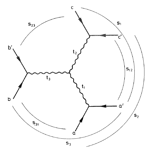
Figure 8: Triple-Regge limit of six-point amplitude.

The variables of Fig. 8 can be expressed in term of BDS variables as follows, (identified in counter clockwise order),

$$t^{[2]}_{a^{\prime}}=s_{12};\;\;t^{[2]}_{c}=s_{23};\;\;t^{[2]}_{b}=s_{31};\;\;t^{[2]}_{a}=t_{1};\;\;t^{[2]}_{c^{\prime}}=t_{2};\;\;t^{[2]}_{b^{\prime}}=t_{3};\;\;t^{[3]}_{a^{\prime}}=s_{1};\;\;t^{[3]}_{a}=s_{2};\;\;t^{[3]}_{b}=s_{3}$$

However only 8 of the 9 variables are independent invariants. Define

$$\eta_{ij}=\frac{s_{ij}}{s_{i}s_{j}}\;.$$ (5.19)

A constraint can be written involving $\eta$’s and $t$’s, and it can be used to eliminate one of the $\eta$’s   [34]. Proceeding as in Sec. 2 and Sec. 4, we find the exact result

$${\cal A}_{6} = \mbox{const}\;A_{tree}\prod^{3}_{i=1}A^{2}_{div}(t_{i})e^{\textstyle\frac{f(\lambda)}{16}[2Q_{6}+\lambda(\log s_{12},\log s_{23},\log s_{31})]}$$ (5.20)

$$\times e^{\textstyle[\frac{f^{(-1)}(\lambda)}{8\epsilon}+\frac{g(\lambda)}{4}][\log(s_{12}/t_{1})+\mbox{cyclic}]+\frac{f(\lambda)}{16}[\log^{2}(t_{1}/\mu^{2})+\mbox{cyclic}]}$$

$$\times e^{\textstyle-\frac{f(\lambda)}{8}[\log(\eta_{13}/\eta_{23})\log(s_{13}/s_{23})+\mbox{cyclic}]+\frac{f(\lambda)}{16}[\log^{2}(\eta_{13}/\eta_{23})+\mbox{cyclic}]}$$

$$\times e^{\textstyle-\frac{f(\lambda)}{8}[{\rm Li}_{2}(1-t_{1}\eta_{23})+{\rm cyclic}]}$$

where $\lambda(a,b,c)=a^{2}+b^{2}+c^{2}-2ab-2bc-2ac$. Note that the cross ratios, which enter through the arguments of the dilogarithms, again remain fixed and finite. One can show again that the $\log^{2}s_{ij}$ type terms in (5.20) cancel. The triple-Regge limit most appropriate to Fig 8 is

$$s_{1},\;\;s_{2},\;\;s_{3},\;\;s_{12},\;\;s_{23},\;\;s_{31}\;-\rightarrow\infty$$

$$t_{1},\;\;t_{2},\;\;t_{3},\;\;\eta_{12},\;\;\eta_{23},\;\;\eta_{31}<0\;,\quad\mbox{fixed}$$ (5.21)

i.e., $u_{1},u_{2},u_{3}$ are again fixed. One finds that (5.20) can again be expressed simply in terms of the gluon Regge trajectory, with the desired triple Regge behavior [34],

$${\cal A}_{6}=\prod^{3}_{i=1}A^{2}_{div}(t_{i})\prod^{3}_{j=1}\left(\frac{-s_{j}}{\mu^{2}}\right)^{\alpha(t_{j})}\;F(t_{i},\eta_{ij})$$ (5.22)

Finally, we note that Regge behavior for 6-point gluon amplitude has also been addressed in [39] from a different perspective.

6 The general BDS $n$-gluon amplitude

We next demonstrate that the findings for $n=6$ in the single-Regge limits and the maximal linear multi-Regge limit can be generalized directly to $n>6$. For $n>6$, type-I single-Regge refer to either $s_{1}$ becoming large or the equivalent limit where $s_{n-3}$ becomes large, whereas type-II will refer to the limit where one of the remaining $s_{k}$’s becoming large.

The BDS formula for general $n$ is ${\cal A}_{n}={\cal A}_{tree,n}M_{n}$,

$$\ln M_{n}=\sum_{i=1}^{n}\ln A_{div}(t_{i}^{[2]})+{\cal F}_{n}^{(1)}(0)\;,$$ (6.1)

where $A_{div}$ is given by (2.8) and ${\cal F}_{n}^{(1)}(0)=(f(\lambda)/8)(Q_{n}+D_{n}+L_{n}+(3n/2)\zeta_{2})$ is obtained from the finite part of the 1-loop ordered n-point amplitude, with

$$Q_{n} = -\sum_{i=1}^{n}\sum_{r=2}^{[n/2]-1}\ln\left(-\frac{t^{[r]}_{i}}{-t^{[r+1]}_{i}}\right)\ln\left(\frac{-t^{[r]}_{i+1}}{-t^{[r+1]}_{i}}\right)$$ (6.2)

and, depending on $n$ even or odd,

$$D_{2m} = -\sum_{i=1}^{2m}\sum_{r=2}^{m-2}{\rm Li}_{2}\left(1-\frac{t^{[r]}_{i}t^{[r+2]}_{i-1}}{t^{[r+1]}_{i}t^{[r+1]}_{i-1}}\right)-\sum_{i=1}^{m}{\rm Li}_{2}\left(1-\frac{t^{[m-1]}_{i}t^{[m+1]}_{i-1}}{t^{[m]}_{i}t^{[m]}_{i-1}}\right)$$ (6.3)

$$L_{2m} = -\frac{1}{4}\sum_{i=1}^{2m}\ln\left(\frac{-t^{[m]}_{i}}{-t^{[m]}_{i+m+1}}\right)\ln\left(\frac{-t^{[m]}_{i+1}}{-t^{[m]}_{i+m}}\right)=\frac{1}{2}\sum_{i=1}^{m}\ln^{2}\left(\frac{-t^{[m]}_{i}}{-t^{[m]}_{i+1}}\right)$$ (6.4)

$$D_{2m+1} = -\sum_{i=1}^{2m+1}\sum_{r=2}^{m-1}{\rm Li}_{2}\left(1-\frac{t^{[r]}_{i}t^{[r+2]}_{i-1}}{t^{[r+1]}_{i}t^{[r+1]}_{i-1}}\right)$$ (6.5)

$$L_{2m+1} = -\frac{1}{2}\sum_{i=1}^{2m+1}\ln\left(\frac{-t^{[m]}_{i}}{-t^{[m]}_{i+m+1}}\right)\ln\left(\frac{-t^{[m]}_{i+1}}{-t^{[m]}_{i+m}}\right)$$ (6.6)

As in the case of $n=6$, we first note the appearance of dilogarithm, with arguments depending on the cross-ratios

$$B_{i,r}=\frac{t^{[r]}_{i}t^{[r+2]}_{i-1}}{t^{[r+1]}_{i}t^{[r+1]}_{i-1}}=\frac{x_{i,j}^{2}x_{i-1,j+1}^{2}}{x_{i,j+1}^{2}x_{i-1,j}^{2}}=u(i,j;i-1,j+1)\;,$$ (6.7)

where $j=i+r$. Note that $B_{i,2}$ is a generalization for $n\geq 6$ of the cross-ratios $u_{1},u_{2},u_{3}$, defined for $n=6$. We will see later another kind of generalized cross-ratio, $u_{k,n}$ ($n=2m$ or $2m+1$), appearing as a constraint in the Regge limits. In the next section cross-ratios will appear in a different context, giving a possible parametrization of the n-point amplitudes. Like for the case of $n=6$, we can show that all these cross-ratios remain bounded in various Regge limits of interests.

In what follows, we will focus on the even amplitudes, $M_{2m}$, $3\leq m$, and, the discussion for $n$ odd, $n=2m+1$, will be also be done in Appendix B. Except for lengthy algebra, nothing note- worthy is found for the odd amplitudes.

We will first analyze the maximal linear multi-Regge limit, where all $s_{i}$, $i=1,2,\cdots,$ $n-3$ are large, and find that we obtain the correct Regge behaviour.

Using the fact that, in the multi-Regge limit, the BDS invariant $t_{i}^{[r]}$, for $2\leq i<i+r\leq n-1$, takes on the factorized form, Eq. (A.15), we show in Appendix B that these cross-ratios approach either $0$ or $1$, just as the case for $n=6$, discussed in Sec. 5. For example, we have, in the multi-Regge limit,

$$B_{1,m-1} = \frac{t^{[m-1]}_{1}t^{[m+1]}_{2m}}{t^{[m]}_{1}t^{[m]}_{2m}}=\left(\frac{t_{m-2}}{t_{m-1}}\right)\left(\frac{t^{[m-1]}_{m+1}}{t^{[m]}_{m}}\right)\simeq\left(\frac{t_{m-2}}{t_{m-1}}\right)\left(\frac{1}{\kappa_{m-1}s_{m-1}}\right)\sim\frac{1}{s_{m-1}}\rightarrow 0$$

$$B_{i,r} = \frac{t^{[r]}_{i}t^{[r+2]}_{i-1}}{t^{[r+1]}_{i}t^{[r+1]}_{i-1}}=\left(\frac{t^{[r]}_{i}}{t^{[r+1]}_{i-1}}\right)\left(\frac{t^{[r+2]}_{i-1}}{t^{[r+1]}_{i}}\right)\simeq\left(\frac{\kappa_{i-1}s_{i-1}}{1}\right)\left(\frac{1}{\kappa_{i-1}s_{i-1}}\right)\rightarrow 1\;,$$ (6.8)

$$\quad\quad\hskip 180.67499pt\;\;3\leq i<i+r\leq 2m-1\;.$$

It follows that these dilogarithms will not affect the leading Regge behaviour. A similar statement applies for the single Regge limits, except there the $B_{i,r}$’s cover what is defined in Appendix A as type 1, 2 and 3 cross-ratios and thus can take on finite values that differ from 0 and 1.

A necessary condition for Regge behaviours is the cancellation of all quadratic terms, both direct, $\ln^{2}s_{j}$, and crossed, $\ln s_{i}\ln s_{j}$, $i\neq j$, $i,j=1,2,\cdots n-3$, for $\log M_{n}$.

Let us first express the contribution from $A_{div}$ as

$$\sum_{i=1}^{2m}\ln A_{div}(t_{i}^{[2]}) = -\frac{f(\lambda)}{16}\left[\sum_{i=1}^{2m-3}\ln^{2}s_{i}+\ln^{2}s\right]+O(1)$$ (6.9)

$$= -\frac{f(\lambda)}{16}\left[\sum_{i=1}^{2m-3}\ln^{2}s_{i}+\ln^{2}(s_{1}s_{2}....s_{2m-3})\right]+O(\ln s_{i})$$

where we have used that, in the multi-Regge limit, the dependent variable $s$ is

$$s\simeq b_{0}\;s_{1}s_{2}....s_{2m-3}$$ (6.10)

where $b_{0}=\Pi_{i=1}^{2m-4}\kappa_{i}$.

We next turn to the contributions from $L_{2m}$. To find them, we need to know how ratios $t_{i}^{[m]}/t_{i+1}^{[m]}$, $1\leq i\leq m$, behave in the multi-Regge limit. Recall, from (A.15), that $t^{[m]}_{i}$ is linear in $s_{j}$ if $j$ falls in the range $[i-1,m+i-3]$. It follows that

$$t^{[m]}_{i}\simeq\beta_{i-1}\;s_{i-1}s_{i}\cdots s_{m+i-4}s_{m+i-3}\;,$$ (6.11)

where $\beta_{i}=\Pi_{j=i}^{m+i-3}\kappa_{j}$, and

$$\frac{t^{[m]}_{i}}{t^{[m]}_{i+1}}\sim\frac{s_{i-1}}{s_{m+i-2}}$$ (6.12)

Since Eq. (6.11) is valid for $2\leq i\leq 2m-r$ and $2\leq r\leq m$, it leads to

$$L_{2m} \simeq \frac{1}{2}\left[\ln^{2}(\frac{t_{m-1}}{s_{1}...s_{m-1}})+\sum_{i=1}^{m-2}\ln^{2}\frac{s_{i}}{s_{m+i-1}}+\ln^{2}(\frac{s_{m-1}s_{m}...s_{2m-3}}{t_{m-1}})\right]+O(\ln s_{i})$$ (6.13)

$$= \frac{1}{2}\left[\sum_{i=1}^{2m-3}\ln^{2}s_{i}+\ln^{2}(s_{1}s_{2}....s_{2m-3})+({\rm crossed\;\;terms})\right]+O(\ln s_{i})$$

where we have made use of the fact that $t_{1}^{[m]}=t^{[m]}_{m+1}=t_{m-1}$. Upon adding $(f(\lambda)/8)L_{2m}$ and $\sum_{i=1}^{2m}\ln A_{div}(t_{i}^{[2]})$, all quadratic terms of the form $\ln^{2}s_{j}$ cancel, leaving only crossed terms as uncanceled contributions to $\ln M_{2m}$,

$$\ln M_{2m} = -\frac{f(\lambda)}{8}\left[\sum_{i=1}^{m-2}\ln s_{i}\ln s_{m+i-1}+\ln(s_{1}...s_{m-2})\ln(s_{m}...s_{2m-3})\right]$$ (6.14)

$$+ \frac{f(\lambda)}{8}Q_{2m}+O(\ln s_{i})\;.$$

For $m=3$, we have

$$\ln M_{6}=-\frac{f(\lambda)}{4}\ln(s_{1})\ln(s_{3})+\frac{f(\lambda)}{8}Q_{6}+O(\ln(s_{i}))\;,$$ (6.15)

which agrees with what we found earlier.

For the contribution from $Q_{2m}$ we need to know how $\ln\frac{t^{[r]}_{i}}{t^{[r+1]}_{i}}\ln\frac{t^{[r]}_{i+1}}{t^{[r+1]}_{i}}$ behaves in the multi-Regge limit. That is, we need to extend (6.11) to $t^{[r]}_{i}$ for $1\leq i\leq 2m-r-1$ and $2\leq r\leq m$, and next to a wider range, i.e., $1\leq i\leq 2m+1$ and $2\leq r\leq m-1$. This is done in Appendix B. ¿From (B.11), we find

$$Q_{2m} \simeq -\sum_{r=2}^{m-1}\left[\sum_{i=1}^{2m-r-2}\ln s_{i}\ln s_{r+i-1}-\ln{s_{1}...s_{2m-r-2}}\ln s_{2m-r-1}\right]$$ (6.16)

$$- \sum_{r=2}^{m-1}\left[\sum_{i=1}^{r-2}\ln s_{i}\ln s_{2m-r+i-1}-\ln s_{r-1}\ln{s_{r}...s_{2m-3}}\right]+O(\ln s_{j})$$

Note that this is a sum of quadratic products, $\ln s_{i}\ln s_{j}$, $i\neq j$. For instance, for $m=3$,

$$Q_{6}\simeq 2\ln s_{1}\ln s_{3}+O(\ln s_{j})\;,$$ (6.17)

which cancels the corresponding term in (6.15). For general $n=2m$, after expanding as a sum over $\ln s_{i}\ln s_{j}$, and after a bit of algebra, these quadratic terms from $Q_{2m}$ cancel exactly against those obtained above, (6.14).

We are now in the position to verify Regge behaviour by finding terms linear in $\ln s_{j}$, thus verifying that the same Regge trajectory function emerges, as dictated by Regge factorization. In order to carry out this analysis, we must keep track of the coefficients of proportionality in (3.16), (6.11), etc. We have done this explicitly in the multi-Regge limit, but the algebra is a bit involved, so we will show some of it in the Appendix. We will instead show this analysis for the single-Regge limits, while leaving out some of the algebraic details. Note that although the algebra is quite different from the multi-Regge case, we in fact obtain the same result for the leading $s_{k}$ behaviour in both cases. If all the single-Regge limits give the expected trajectories, the multi-Regge behaviour will also give the correct result.

We thus finally obtain that

$$\ln M_{2m}\simeq\sum_{k=1}^{2m-3}(\alpha(t_{k})-1)\ln(-s_{k})+O(1)$$ (6.18)

A similar analysis can also be carried out for the $O(1)$ terms. It follows that $M_{2m}$ can now be put into the expected multi-Regge power law behaviour, (3.19). Details of this analysis, together with that for $n=2m+1$, are shown in Appendix B.

We now address the single Regge limits. In the case of $n=6$, we have distinguished two types of single-Regge limits. For type-I, one of the two vertices is elastic, involving only two particles. We will provide a unified treatment here where an arbitrary $s_{k}$ goes to infinity, with other $s_{r}$’s fixed. Because of symmetry, we can restrict to $1\leq k\leq m-1$, and type-I Regge corresponds to $k=1$.

To be precise, the single-Regge limit now corresponds to

$$s_{k}\rightarrow-\infty,$$ (6.19)

with $t_{i}$, $\kappa_{j}$, and all other $s_{l}$ negative and fixed. As discussed in Sec. 3 and in Appendix A, those BDS invariants, $t_{i}^{[r]}$, which “cross” the Regge line, labelled by $t_{k}$, (see Figs. 2 and 3), will also go to infinity. That is, $t_{i}^{[r]}\rightarrow\infty$, with $\frac{t_{i}^{[r]}}{s_{k}}$ fixed,

$${\rm for}\;\;2\leq i\leq k+1\;\;,\quad\quad{\rm if}\quad k+3\leq i+r\leq 2m$$

$${\rm for}\;\;k+2\leq i\leq 2m\;\;,\quad\quad{\rm if}\quad 2\leq i+r-2m\leq k+1\;.$$ (6.20)

In particular, the dependent variable $s$ also goes to infinity, with $s/s_{k}$ fixed.

With these preliminaries, we now repeat what we have done earlier in the cancellation of the quadratic term, $\ln^{2}s_{k}$, while keeping track of terms linear in $\ln s_{k}$. From $L_{2m}$ and $A_{div}$, the $\ln^{2}s_{k}$ term indeed cancels, and we obtain, (after a bit of algebra), the contribution to $\ln M_{2m}$ which is linear in $\ln s_{k}$,

$$\left[\frac{f(\lambda)}{8}\ln\left(\frac{t_{2}^{[m]}t^{[m]}_{k+1}\mu^{4}}{t_{m-1}ss_{k}t_{k+2}^{[m]}}\right)+\frac{g(\lambda)}{2}+\frac{f^{-1}(\lambda)}{4\epsilon}\right]\ln s_{k}$$ (6.21)

The analysis of the terms coming from $Q_{2m}$ is understandably quite involved, and we will not reproduce it here. As expected, it does not contain a $\ln s_{k}^{2}$ term, and the result is a contribution $O(\ln s_{k})$

$$\frac{f}{8}\ln\left[\left(\frac{\mu^{2}}{-t_{k}^{2}}\right)\left(\frac{t_{m-1}s_{k}st_{k+2}^{[m]}}{t_{2}^{[m]}\mu^{4}t_{k+1}^{[m]}}\right)\left(\frac{s_{k}s}{t_{2}^{[k+1]}t_{2m}^{[k+1]}}\right)\right]\ln s_{k}$$ (6.22)

Adding up these two contributions, we obtain, after re-expressing $s_{k}=t_{k+2}^{[2]}$ and $s=t_{2}^{[2m-2]}$

$$\ln M_{2m}\simeq(\alpha(t_{k})-1)\ln s_{k}+\frac{f}{8}\;\ln\left(\frac{t_{k+1}^{[2]}\;t_{2}^{[2m-2]}}{t_{2}^{[k+1]}t_{2m}^{[k+1]}}\right)\ln s_{k}$$ (6.23)

For the type-I single-Regge limit, with $k=1$ (or $k=2m-3$), the last factor cancels identically, and, as in the case of $n=6$, we obtain the desired Regge trajectory.

Next consider type-II single-Regge. Note that the combination in the last term is a cross-ratio, $2\leq k\leq 2m-4$, (a different generalization of $u_{3}$ to the case of $n\geq 6$ than $B_{i,r}$)

$$u_{k,2m}=\frac{t_{2}^{[2m-2]}\;t_{k+1}^{[2]}}{t_{2}^{[k+1]}t_{2m}^{[k+1]}}=u(2,2m;k+1,k+3)\;.$$ (6.24)

For $m=3$ and $k=2$, one easily verify that $u_{2,6}=u_{3}$ introduced in (5.7). Since this cross-ratio approaches 1 in the single-Regge limit (see eq. (A.11)),

$$u(2,2m;k+1,k+3)\rightarrow 1$$ (6.25)

it follows that

$${\cal A}_{2m}\sim\left(\frac{s_{k}}{t_{k}}\right)^{\alpha(t_{k})}$$ (6.26)

for both type-I and type-II single Regge limits, as advertised. The same cross-ratio constraint, $u_{k,2m}\rightarrow 1$ appears in the Regge trajectory for the multi-Regge limit.

7 Regge behaviour and dual conformal symmetry

In this section we describe the interplay between Regge behaviour of the n-gluon amplitude and the solution of the conformal Ward identities for the n-cusp Wilson loop [7]. Drummond et al. [4] and Brandhuber et al. [5] proposed a duality between the n-sided polygon Wilson loops and the n-point gluon amplitudes, in part from a perturbative analysis for n=4,5 [4] and general n [5]. At 1 loop, the duality is found to be exact. Further, the Alday and Maldacena proposal [3] for the strong coupling gluon amplitude implies the validity of the duality as a consequence of the trivial geometric equality of the AdS space (where one calculates the minimal surface of the Wilson loop) and of the T-dual AdS space (where one calculates the minimal surface giving the gluon amplitude). However, to define the Wilson loop or its dual one needs a regulator, which makes the duality less trivial. This duality is also broken at finite temperature [14].

Drummond et al. [6, 7] further proved a conformal Ward identity for the polygon Wilson loops for all orders in perturbation theory. Recently Komargodski [40] proved the anomalous Ward identity of Drummond et al. for the strong- coupling (AM) dual of the gluon amplitude. One writes the expectation value of the Wilson loop $W(C_{n})$ as

$$\ln W_{n}(C_{n})=Z_{n}+F_{n}^{(WL)}$$ (7.1)

which separates the divergent factor $Z_{n}$ from the finite part of the Wilson loop, and $C_{n}$ is the same contour that appears in (1.1). They propose that

$$\sum_{i=1}^{n}(2x_{i}^{\mu}x_{i}\cdot\partial_{i}-x_{i}^{2}\partial_{i}^{\mu})F_{n}^{(WL)}=\frac{1}{2}\Gamma_{cusp}(\lambda)\sum_{i=1}^{n}\ln\left(\frac{x_{i,i+2}^{2}}{x_{i-1,i+1}^{2}}\right)x_{i,i+1}^{\mu}$$ (7.2)

where

$$x^{2}_{i,i+r}=(k_{i}+...+k_{i+r-1})^{2};\;\;\;\;k_{i}=x_{i}-x_{i+1}$$ (7.3)

thus $x_{i,i+r}^{2}$ is $t_{i}^{[r]}$ in the case of the dual gluon amplitude, and $\Gamma_{cusp}=Cf(\lambda)$ is the cusp anomalous dimension that appears in the previous sections. The most general solution to (7.2) for n=4 and n=5 is

$$F_{4}^{(WL)}=F_{4}^{(BDS)}+{\rm constant};\;\;\;\;\;\;F_{5}^{(WL)}=F_{5}^{(BDS)}+{\rm constant}$$ (7.4)

where

$$\exp F_{n}^{(BDS)}=[A_{n}^{(BDS)}]_{finite}$$ (7.5)

Equation (7.4) lends support to the BDS conjecture for n=4 and 5, and led to the proposed duality between the n-cornered Wilson loop and the n-gluon amplitude.

The general solution of (7.2) for n=6 is

$$F_{6}^{(WL)}=F_{6}^{(BDS)}+f(u_{1},u_{2},u_{3})$$ (7.6)

where $f(u_{1},u_{2},u_{3})$ is an arbitrary function of the three cross-ratios

$$u_{1}=\frac{x_{13}^{2}x_{46}^{2}}{x_{14}^{2}x_{36}^{2}};\;\;\;u_{2}=\frac{x_{24}^{2}x_{15}^{2}}{x_{25}^{2}x_{14}^{2}};\;\;\;u_{3}=\frac{x_{35}^{2}x_{26}^{2}}{x_{36}^{2}x_{25}^{2}}$$ (7.7)

It is important to note that the dilog terms $D_{6,i}$ in (5.4) are functions of the cross-ratios only, as we saw already in (5.7), and as such do not contribute to the right-hand side of (7.2). Recently, Drummond et al. [10] found that in general $f(u_{1},u_{2},u_{3})\neq$ constant, from a two-loop calculation of $F_{6}^{(WL)}$.

Now consider (7.2) from the point of view of this paper, where we claim that the Regge and multi-Regge behaviour of the n-gluon amplitudes is a necessary property of the theory. Note that the dilog terms, $D_{6}$, in the last line of (5.20) are finite and nonzero in the various Euclidean Regge limits considered in Sec. 5. This observation then generalizes to the fact that in the single-Regge limits and triple-Regge limits, it is plausible that

$$f(u_{1},u_{2},u_{3})={\rm finite}$$ (7.8)

in the Euclidean region for any function of the cross-ratios, as the cross-ratios are finite in these limits. Taking (7.6) together with (7.8), this implies that $F^{WL}_{6}$ has the same Regge and behaviour as $F_{6}^{(BDS)}$, where $F_{6}^{WL}$ is the solution of (7.2).

The line of argument in the preceding paragraphs generalizes to $n>6$. Using the results of [7], we obtain that the solution to (7.2) for $n\geq 7$ is

$$F_{n}^{(WL)}=F_{n}^{(BDS)}+f(u_{1},u_{2},...,u_{p})$$ (7.9)

where $f(u_{1},...,u_{p})$ is an arbitrary function of the distinct cross-ratios. It is shown in Sec. 6 that the Regge limits of $F_{n}^{(BDS)}$ have the expected Regge behavior in the Euclidean region. For example, the function of cross ratios $B_{i,r}$, (6.7), (generalizations of $u_{1},u_{2},u_{3}$ for $n\geq 7$) remain finite in the limit leading to (6.26). We therefore conclude that the Euclidean Regge limits considered in this paper do not distinguish between $F_{n}^{WL}$, $F_{n}^{BDS}$, and $F_{n}$, where the latter is the actual n-gluon amplitudes. Further, if the functions of the cross-ratios in (7.6) and (7.9) remain finite in the Regge limits, then $F_{n}^{(WL)}$ is also not distinguished from $F_{n}^{BDS}$ by Regge behavior in the Euclidean region.

8 Concluding remarks

It is expected that ${\cal N}=4$ SYM theory exhibits stringy properties, albeit with infinite string tension as required by the conformal symmetry of the theory. This view is based on the ’t Hooft $1/N$ expansion, as well as the AdS/CFT correspondence. Indeed Alday and Maldacena have used the AdS/CFT correspondence for the Wilson loop in strong coupling to predict the color-ordered n-gluon scattering amplitude for large N, $SU(N)$ ${\cal N}=4$ SYM theory. For the 4-point function, the AM construction is in agreement with the BDS conjecture for the 4-gluon MHV planar scattering amplitude. Further it has been shown that the $n=4$ amplitude can be cast exactly as a Regge amplitude with a large N Regge trajectory function valid to all orders in perturbation theory, presented in (2.6).

In this paper we have examined the Regge and multi-Regge behavior of the BDS conjecture for $n\geq 5$ in the Euclidean region. It was found that the BDS conjecture is consistent with the Regge limit taken in this region. A crucial tool in this conclusion is an understanding of the behavior of various cross- ratios in Regge limits.

It is known from the recent work of Drummond et al.[10] that the hexagonal Wilson loop differs from the BDS conjecture for the 6-gluon amplitude by a non-constant function of the three cross- ratios. Given the basic assumption of this paper, that the n-gluon amplitudes should exhibit Regge and multi-Regge behaviour, we showed in section 7 that if the function in (7.6) and (7.9) remain finite in the Regge limits, then Regge behavior in the Euclidean region does not distinguish between $F_{n}^{WL}$, $F_{n}^{(BDS)}$, or $F_{n}$ where $F_{n}$ is the n-gluon amplitude. Continuation to the physical region enables one to examine this issue further [41, 42].

We should emphasize that there is considerably more that can be done using Regge limits to test and constrain conjectures for the n-point ${\cal N}=4$ SYM amplitudes. We have not exhausted the full repertoire of limits determined by the Regge hypothesis or considered the analytic continuation to the physical region, or the full constraints of factorization and analyticity on residue functions. For example, we have not discussed the constraints of overlapping singularities and the issue of analyticity in $\kappa_{i}$, an important but subtle issue [28, 34, 38], as well as the crossing relations in other related multi-Regge limits [38] which can play a significant role in the BFKL program [43, 44] for the high energy limit of ${\cal N}=4$ SYM in the vacuum channel with cylinder topology [29, 30, 31]. Also for $n\geq 6$, we have not investigated contributions below the leading trajectory, which in the planar limit are expected to be simple poles in the $J$-plane, free of Regge cuts.

Finally, given the crucial role played by the various cross-ratios and their limits in our analysis, one may conjecture that the limits of cross-ratios are a central issue to be addressed in achieving Regge behavior in any conformal theory, and perhaps other theories as well.

Note added: 

Since the appearence of this paper (BNST-I) on the archives, there have been several papers extending the present investigation [41, 42, 45, 46] in interesting directions. While they generally go beyond the scope of this article, they do contribute valuable additional information of relevance to the underlying question of Regge properties for BDS amplitudes. In particular, these papers have considered the important issue of the multi-Regge behavior continued into the physical region. In Ref. [41], which was posted shortly after our paper appeared, Bartels, Lipatov and Sabio Vera (BLSV-I) studied the linear multi-Regge behavior for six-gluon amplitudes in the physical region. For certain color configurations, non-factorization was found. The issue of analytic continuation back to the physical scattering region for all relevant color configurations is also the focus of our subsequent paper [42] on Regge limits of BDS (BNST-II). We compare and contrast features of the BDS amplitudes with that from flat-space string theory, paying particular attention to proper handling of threshold singularities of multi-Regge amplitudes, thus maintaining causality relations in the course of continuation back to the physical region.

The continuation discussed by BLSV-I involves expanding in the dimensional regulator $\epsilon\rightarrow 0$ and then analytically continuing the finite part of the 1-loop amplitude (that appears in the exponent of the BDS ansatz) according to a causal prescription. The BLSV-I continuation among other things leads to a subtle diverging term $\sim 2\pi i\ln(1-u_{3})$, where $u_{3}$ is a conformally invariant cross-ratio approaching 1 in the Regge limit, as well as an extra term, which is not a function of conformally invariant cross-ratios. As it stands, the BLSV-I continuation does not permit “naive factorization” in the form of Eq. (5.17) of our paper. There are many subtleties, some of which we discuss in [42]. For example, we note that, for flat-space string theory, physical region factorization in the multi-Regge limit applies only to amplitude of definite “signature”, not to specific subset of planar amplitudes identified in BLSV-I as non-factorizable. Further analysis was carried out in BLSV-II [46]. We also note that a paper by Del Duca, Duhr and Glover [45] appeared after [42]. They have considered the possibility of analytical continuation with $\epsilon\neq 0$ fixed, taking the Regge limit before the $\epsilon\rightarrow 0$ limit, which leads to a result differing from that of BLSV-I. In their approach, the anomalous term of BLSV-I does not appear. Further discussion of these issues will be addressed in an updated version of BNST-II.

Finally the results of Bern et al. [47] and Drummond et al. [48] are also interesting in the present context. They show numerically that the BDS ansatz for the six-gluon amplitude fails for finite (non-limiting) kinematics. On the other hand, the duality between MHV amplitudes and Wilson-loops have been shown to hold to 2 loops and 6 external legs, (for the parity even part in [47, 48], for the parity odd part in [49].) In view of the theorems (both all-loop perturbative [7] and strong coupling [40]) proving dual conformal symmetry of the Wilson-loop, the deviation from the 6-gluon BDS amplitudes that was found in [47, 48] must be a function of cross-ratios. It is also worth noting that Refs. [50, 51] proved that dual conformal symmetry arises from a combination of bosonic plus fermionic T dualities, and [52] embedded dual conformal symmetry in dual superconformal symmetry.

Acknowledgements: The work of RCB was supported by the Department of Energy under Contract. No. DE-FG02-91ER40676. HN would like to thank Katsushi Ito and Alexei Morozov for discussions. HN’s research has been done with partial support from MEXT’s program ”Promotion of Environmental Improvement for Independence of Young Researchers” under the Special Coordination Funds for Promoting Science and Technology. HJS wishes to thank Lance Dixon for conversations and correspondence. He also wishes to acknowledge the stimulating atmosphere of the 2007 Brown string meeting, which played an important role in forming this collaboration. HJS’s research is supported in part by the DOE under grant DE- FG02-92ER40706. CIT would like to thank E. M. Levin for discussion and prior collaboration and also thank G. Korchemski for correspondence. His research is supported in part by the U. S. Department of Energy under Contract DE-FG02-91ER40688, TASK A. In particular, we would like to thank Marcus Spradlin and Anastasia Volovich for pointing out a crucial error in the original version of this manuscript.

Appendix A BDS variables and constraints

In this Appendix we describe the variables used by BDS and constraints between them, in general and in the Regge limits, as well as a parametrization for them used in the multi-Regge limit in the text.

The variables used by BDS are $t_{i}^{[r]}\equiv(k_{i}+...+k_{i+r-1})^{2}$ or $x_{i,i+r}^{2}$ in the Wilson loop dual notation of [7]. (All indices are defined mod n.) There are $n(n-3)/2$ such cyclic invariants, since momentum energy conservation implies $t_{i}^{[r]}=t^{[n-r]}_{i+r}$. However, the number of independent Lorentz invariant parameters in the amplitude should be $3n-10$ (a simple way to see this is that there are 2 parameters for the 4-point amplitude, $s$ and $t$, and each new on-shell momentum adds another 3). That means that only the 4-point and 5-point amplitudes (when $n(n-3)/2=3n-10$) are described by independent $t_{i}^{[r]}$’s (2 and 5 of them, respectively), for $n>5$ there are constraints between them.

To understand these constraints, we first look at the first nontrivial case, the 6-point amplitude. Then there are 9 $t_{i}^{[r]}$ variables, but there should be 8 parameters, so there is one constraint between them. The variables can be chosen to be $t_{i}^{[2]},i=1,...,6$ and $t_{1}^{[3]},t_{2}^{[3]},t_{3}^{[3]}$.

Now let us describe the constraint. Since we have a 6-point amplitude, there are 6 momenta $k_{i}$, but momentum conservation fixes one of them, e.g. $k_{6}=-(k_{1}+...+k_{5})$, so there are 5 momenta that can be independently varied. But invariance under the Poincare group restricts further the number of parameters appearing in the amplitude. Since we are in a 4 dimensional space, the 5 momenta must be linearly dependent. Therefore $\exists\alpha_{i}$ constants such that $\sum_{i}\alpha_{i}k_{i}=0$ (4 equations for the 4 components). Multiplying with $k_{j}$ we get 5 dependent equations, therefore

$$P_{5}\equiv\det M_{ij}=0;\;\;\;M_{ij}\equiv(k_{i}\cdot k_{j}),\;\;i,j=1,..,5$$ (A.1)

This is a constraint equation in terms of $k_{i}\cdot k_{j}$, but it turns out that all of them can be expressed in terms of $t_{i}^{[r]}$’s. Since $k_{i}^{2}=0$, we have

$$t_{i}^{[r]}=\sum_{i\leq l,m\leq i+r-1}k_{l}\cdot k_{m}$$ (A.2)

and in particular $t_{i}^{[2]}=2k_{i}\cdot k_{i+1}$ for $i=1,..,4$. In addition, we have

$$2k_{1}\cdot k_{3}=t_{1}^{[3]}-t_{1}^{[2]}-t_{2}^{[2]}; 2k_{2}\cdot k_{4}=t_{2}^{[3]}-t_{2}^{[2]}-t_{3}^{[2]}$$

$$2k_{3}\cdot k_{5}=t_{3}^{[3]}-t_{3}^{[2]}-t_{4}^{[2]}; 2k_{5}\cdot k_{1}=t_{2}^{[3]}-t_{5}^{[2]}-t_{6}^{[2]}$$

$$2k_{1}\cdot k_{4}=t_{2}^{[2]}+t_{5}^{[2]}-t_{1}^{[3]}-t_{2}^{[3]}; 2k_{2}\cdot k_{5}=t_{3}^{[2]}+t_{6}^{[2]}-t_{2}^{[3]}-t_{3}^{[3]}$$ (A.3)

These complete the 10 nontrivial elements of $M_{ij}$, thus $P_{5}$ is expressed as a homogeneous polynomial of degree 5 in the $t_{i}^{[r]}$ variables. In principle it could be an identity (i.e., $P_{5}\equiv 0$) and not a constraint, but expanding it explicitly shows it is indeed a constraint. We will not reproduce it here, since it will fill half a page and we would learn nothing new.

We now turn to the general case of an $n>5$ point amplitude. We need $(n-4)(n-5)/2=\begin{pmatrix}n-4&\\ 2&\\ \end{pmatrix}$ constraints, obtained in a similar way. Among the $n$ momenta pick a basis for 4 dimensional space, say $k_{1},k_{2},k_{3},k_{4}$. ¿From the remaining $n-4$ momenta, pick one to be expressed from the others by momentum conservation, e.g. $k_{n}=-(k_{1}+...+k_{n-1})$, and call it $k_{i}$. Then pick another one, $k_{j}$, who will be expressed as a linear combination of the basis $k_{1},..,k_{4}$. As above, we obtain the constraint $\det M_{i^{\prime\prime}j^{\prime\prime}}=0$, $M_{i^{\prime\prime}j^{\prime\prime}}=k_{i^{\prime\prime}}\cdot k_{j^{\prime\prime}}$, where $i^{\prime\prime}\in(1,2,3,4,j)$.

Now $2k_{i^{\prime}}\cdot k_{j^{\prime}}$, where $i^{\prime}=1,...,n$ except $k_{i}$, can be expressed as a linear combination of the $t_{i}^{[r]}$’s as we did for the 6- point amplitude, i.e.

$$2k_{i^{\prime}}\cdot k_{j^{\prime}}=\sum_{r,k}\alpha_{r,k}t_{k}^{[r]}$$ (A.4)

This can be seen as follows. There are $n(n-1)/2$ nontrivial values for $k_{l}\cdot k_{m}$, l,m=1,…n, since $k_{i}^{2}=0$ (thus $l=m$ is excluded). By picking out $k_{i}$ and writing it as minus the sum of the other momenta (by momentum conservation), we can express $n-1$ of the $k_{l}\cdot k_{m}$ variables as a function of the others, and we are left with $(n-1)(n-2)/2=n(n-3)/2+1$ independent ones. But we still have one constraint left

$$\sum_{i^{\prime},j^{\prime}=1,i^{\prime},j^{\prime}\neq i}^{n}k_{i^{\prime}}\cdot k_{j^{\prime}}=(\sum_{i^{\prime}=1,i^{\prime}\neq i}^{n}k_{i^{\prime}})^{2}=(-k_{i})^{2}=0$$ (A.5)

therefore we can eliminate another one of the $k_{i^{\prime}}\cdot k_{j^{\prime}}$ as a function of the others, and we are left with $n(n-3)/2$, exactly the number of variables $t_{i}^{[r]}$. That means that we can now invert the relation (A.2) and obtain (A.4).

Therefore, the polynomial constraint $\det M_{i^{\prime\prime}j^{\prime\prime}}=0$ is again expressed in terms of the $t_{i}^{[r]}$’s. But we needed to pick two momenta, $i$ and $j$, out of the $n-4$ dependent ones, therefore we can do this in $(n-4)(n-5)/2$ ways, obtaining the needed $(n-4)(n-5)/2$ constraints (actually, choosing first $i$ and then $j$ or vice versa seems to be different, but by considering only one case we already obtain all the needed constraints, therefore the reversed case will give the same).

In conclusion, the variables $t_{i}^{[r]}$ are restricted by $(n-4)(n-5)/2$ complicated 5-th order polynomial constraints. This will be cumbersome for the treatment of limits of $n$-point amplitudes. Luckily, in the Regge limits, the constraints greatly simplify, and one can deal with them systematically.

As described in the text, in the linear multi-Regge limit one can choose a set of $3n-10$ independent parameters among the $t_{i}^{[r]}$’s that describe the physics well, specifically

$$s_{i}=t_{i+1}^{[2]},\;i=1,...,n-3\;\;\;\hskip 28.45274ptt_{r}=t_{1}^{[r+1]}=t_{r+2}^{[n-r-1]},\;r=1,...,n-3$$ (A.6)

and

$$\Sigma_{i}=t_{i+1}^{[3]},\;i=1,...,n-4$$ (A.7)

that describe the limit as in Fig.2. The advantage is that they can be varied independently, and the behaviour of the rest of the $t_{i}^{[r]}$’s can be found in terms of them. Some constraints become easy to write down in the Regge limits.

We now show a systematic way to find such constraints in the single Regge limit, for $s_{k}\rightarrow\infty$. They are related with the definition of the generalized cross ratios, whose usefulness we have found throughout this paper.

The Regge line for $s_{k}$ separates the momenta into right movers $k_{i}^{+}\rightarrow\infty$ (for momenta on the left of the line) and left movers $p_{j}^{-}\rightarrow\infty$ (for momenta on the right of the line). Cross ratios correspond to two momentum invariants divided by other two momentum invariants, and can be described as falling into 3 classes, in the $s_{k}$ single Regge limit:

• 1. All 4 momentum invariants involve either only right ($k$’s) or only left ($p$’s) momenta.

• 2. In two of the 4 invariants we have both left and right momenta.

• 3. All 4 momentum invariants involve both left and right momenta.

Type-1 cross ratios are finite variables, and obviously appear either in the left or the right factorized function in the Regge limit.

Type-2 cross ratios also become finite variables of only the right-moving or left-moving momenta, thus appear in either the left or right factorized function in the Regge limit. For concreteness, we will look at the case where the variables are on the left. Define

$$u(i,j;p,q)=\frac{(k_{i}+...+k_{j-1})^{2}(k_{p}+...+k_{q-1})^{2}}{(k_{i}+...+k_{q-1})^{2}(k_{p}+...+k_{j-1})^{2}}=\frac{x_{i,j}^{2}x_{p,q}^{2}}{x_{i,q}^{2}x_{p,j}^{2}}$$ (A.8)

where $2\leq i<p<q-1\leq k+1<j-1\leq n-1$. Also define $P^{\mu}=\sum_{r=i}^{k+1}k_{r}^{\mu}$, $Q^{\mu}=\sum_{r=k+2}^{j-1}k_{r}^{\mu}$ and $p^{\mu}=\sum_{r=p}^{k+1}k_{r}^{\mu}$. Then in the limit,

$$u(i,j;p,q)\simeq\frac{(k_{p}+...k_{q-1})^{2}(P^{+}Q^{-})}{(k_{i}+...k_{q-1})^{2}(p^{+}Q^{-})}=\frac{(k_{p}+...k_{q-1})^{2}P^{+}}{(k_{i}+...k_{q-1})^{2}p^{+}}$$ (A.9)

which is a finite function of only right-moving variables, as stated.

Type-3 cross ratios are the important ones, that will give constraints. We define similar variables

$$u(i,j;p,q)=\frac{(k_{i}+...+k_{j-1})^{2}(k_{p}+...+k_{q-1})^{2}}{(k_{i}+...+k_{q-1})^{2}(k_{p}+...+k_{j-1})^{2}}=\frac{x_{i,j}^{2}x_{p,q}^{2}}{x_{i,q}^{2}x_{p,j}^{2}}$$ (A.10)

but where now $2\leq i<p<q-1<j-1\leq n-1$, and $p\leq k+1,k+2\leq q-1$, and $P^{\mu}=\sum_{r=i}^{k+1}k_{r}^{\mu}$, $Q^{\mu}=\sum_{r=k+2}^{j-1}k_{r}^{\mu}$, $p^{\mu}=\sum_{r=p}^{k+1}k_{r}^{\mu}$, $q^{\mu}=\sum_{r=k+2}^{q-1}k_{r}^{\mu}$, we get in the limit

$$u(i,j;p,q)\simeq\frac{(P^{+}Q^{-})(p^{+}q^{-})}{(P^{+}q^{-})(p^{+}Q^{-})}=1$$ (A.11)

which therefore represents a constraint, that has been used in the text.

Further kinematic simplifications can be achieved in the linear multi-Regge limit, where, after supplying a minus sign for each out-going longitudinal momenta,

$$-k_{2}^{+}>>-k_{3}^{+}>>\cdots-k_{i}^{+}>>\cdots>>-k_{n-2}^{+}>>-k_{n-1}^{+}$$ (A.12)

In this limit, for $2\leq i<j\leq n$,

$$x_{i,j}^{2}=t_{i}^{[j-i]}=(\sum_{r=i}^{j-1}k_{r})^{2}\simeq 2(\sum_{r}k_{r})^{+}(\sum_{r}k_{r})^{-}\simeq 2k^{+}_{i}k^{-}_{j-1}+O(1)\;.$$ (A.13)

(When $i=1$, $x_{1,j}^{2}=t_{j}$, which is fixed in this limit, and above approximation is no longer valid.) It follows that we can derive a recursive relation for invariants $t_{i}^{[r]}=[i,i+r]$,

$$t_{i+1}^{[j-i+2]}\simeq s_{i}\kappa_{i}\;t_{i+2}^{[j-i+1]}\;,\quad t_{i+1}^{[j-i+2]}\simeq t_{i+1}^{[j-i+1]}\;s_{j}\kappa_{j-1}\;,$$ (A.14)

for $1\leq i<j\leq n-3$, and from which one has

$$[i,j]=t_{i}^{[j-i]}=\kappa_{i-1}\kappa_{i}\cdots\kappa_{j-4}s_{i-1}s_{i}\cdots s_{j-4}s_{j-3}$$ (A.15)

This also means that, in this limit,

$$s\simeq\kappa_{1}\kappa_{2}\cdots\kappa_{n-4}{s_{1}s_{2}\cdots s_{n-3}}$$ (A.16)

as mentioned in Sec. 3, Eq. (3.16).

Appendix B Regge Limits for $n>6$: details

Here we provide details which have been left out of Sec. 6. We begin with the treatment of the linear multi-Regge limit. We first discuss how kinematic constraints in the multi-Regge limit can be used to study the dilogarithms terms in (6.3) and (6.5), which depend on the generalized cross-ratios $B_{i,r}$. We show specifically that $B_{i,r}$ remain bounded in the linear multi-Regge limit. We have

$$B_{i,r}=u(i,i+r;i-1,i+r+1)=\frac{x_{i,i+r}^{2}x_{i-1,i+r+1}^{2}}{x_{i,i+r+1}^{2}x_{i-1,i+r}^{2}}=\frac{t^{[r]}_{i}t^{[r+2]}_{i-1}}{t^{[r+1]}_{i}t^{[r+1]}_{i-1}}$$ (B.1)

where $D_{n}$ for n even and odd can be expressed as

$$D_{2m} = -\sum_{i=1}^{2m}\sum_{r=2}^{m-2}{\rm Li}_{2}\left(1-B_{i,r}\right)-\sum_{i=1}^{m}{\rm Li}_{2}\left(1-B_{i,m-1}\right)$$ (B.2)

$$D_{2m+1} = -\sum_{i=1}^{2m+1}\sum_{r=2}^{m-1}{\rm Li}_{2}\left(1-B_{i,r}\right)$$ (B.3)

Note that $B_{i,2}$ becomes $u_{1},u_{2},u_{3}$ (5.7) for $n=6$, thus $B_{r,i}$ are generalizations for $n\geq 6$ and $1\leq i\leq n$ of these variables, analyzed in Sec. 3.

We will first analyze the n=2m case. The behaviour for some of the cross ratios can be found easily, e.g., using (A.15). More directly, using (A.13), we get

$$B_{i,j-i} = \frac{x_{i,j}^{2}x_{i-1,j+1}^{2}}{x_{i,j+1}^{2}x_{i-1,j}^{2}}\simeq\frac{(k_{i}^{+}k_{j-1}^{-})(k_{i-1}^{+}k_{j}^{-})}{(k_{i}^{+}k_{j}^{-})(k_{i-1}^{+}k_{j-1}^{-})}=1\;,$$ (B.4)

provided that $i,i-1,j,j-1\neq 1$. Thus all cross-ratios in (B.2) and (B.3), approach

$$B_{i,r}\rightarrow 1\;,$$ (B.5)

with the exception of those involving $x_{1}$. (When the initial momenta $k_{1}$ and $k_{n}$ enter, the approximation, Eq. (A.13) is no longer valid.) For $B_{i,m-1}$, $1\leq i\leq m$, the allowed special cases are $i=1$ and $i=2$, giving $u(1,r+1;2m,r+2)$ and $u(2,r+2;1,r+3)$ respectively. Like the cross-ratios $u_{1}$ and $u_{2}$, they vanish in the multi-Regge limit. Explicitly, we find from (A.15),

$$B_{1,m-1}=\left(\frac{t_{m-2}}{t_{m-1}}\right)\left(\frac{t^{[m-1]}_{m+1}}{t^{[m]}_{m}}\right)\sim\frac{1}{s_{m-1}}\rightarrow 0;\;\;\;\;B_{2,m-1}=\left(\frac{t_{m}}{t_{m-1}}\right)\left(\frac{t^{[m-1]}_{2}}{t^{[m]}_{2}}\right)\sim\frac{1}{s_{m-1}}\rightarrow 0$$ (B.6)

For $B_{i,r}$, one of $i,i-1,i+r,i+r-1$ being $1$, gives $i=1,2,2m-r,2m-r+1$, with $2\leq r\leq m-2$. We find, again using (A.15),

$$B_{1,r}=\left(\frac{t_{r-1}}{t_{r}}\right)\left(\frac{t^{[r+2]}_{2m}}{t^{[r+1]}_{2m}}\right)\sim\frac{1}{s_{r}}\rightarrow 0,\;\;\;\;B_{2,r}=\left(\frac{t_{r+1}}{t_{r}}\right)\left(\frac{t^{[r]}_{2}}{t^{[r+1]}_{2}}\right)\sim\frac{1}{s_{r}}\rightarrow 0,$$

$$B_{2m-r,r}=\left(\frac{t_{2m-r-3}}{t_{2m-r-2}}\right)\left(\frac{t^{[r]}_{2m-r}}{t^{[r+1]}_{2m-r-1}}\right)\sim\frac{1}{s_{2m-r-2}}\rightarrow 0,$$

$$B_{2m-r+1,r}=\left(\frac{t_{2m-r-1}}{t_{2m-r-2}}\right)\left(\frac{t^{[r+2]}_{2m-r}}{t^{[r+1]}_{2m-r}}\right)\sim\frac{1}{s_{2m-r-2}}\rightarrow 0\;.$$ (B.7)

We therefore have shown that $B_{m-1,i}$ and $B_{r,i}$ are bounded in the multi-Regge limit (they approach either 1 or 0). Therefore $D_{2m}$ remains finite and the dilog’s in (B.2) will not affect the leading behavior for $\ln M_{2m}$.

As described in section 3 and the Appendix A, it is convenient to specify the BDS variables by $t_{i}^{[r]}$ for $r<m$, $i=1,...,2m$, and $t^{[m]}_{i}$ for $i=1,...,m$. However, there are constraints among them. A set of $3n-10$ independent invariants can be taken to be $s_{i}=t_{i+1}^{[2]}$ for $i=1,...,2m-3$, $t_{r}=t_{1}^{[r+1]}=t_{r+2}^{[n-r-1]}$ for $r=1,...,2m-3$, and $\Sigma_{i}=t_{i+1}^{[3]}$ for $i=1,...,2m-4$. (Equivalently, instead of $\Sigma_{i}$, we can use $\kappa_{i}=\Sigma_{i}/s_{i}s_{i+1}$.) This set is most convenient for describing the maximal linear multi-Regge limit, where $s_{i}$ and $\Sigma_{i}$ are going to infinity, with $t_{i}$ and $\kappa_{j}$ fixed. ¿From the constraint (A.16), $s$, as a dependent variable, also goes to infinity, with the following ratio fixed

$$b_{0}=\frac{s}{s_{1}...s_{2m-3}}\simeq\kappa_{1}\kappa_{2}\cdots\kappa_{2m-4}\;.$$ (B.8)

In order to understand how contributions from $L_{2m}$ and $Q_{2m}$ behave in various Regge limits, we need to know the behaviour of all $t_{i}^{[r]}$’s. First, $t_{1}^{[r]}=t_{r+1}^{[2m-r]}=t_{r-1}$ is fixed. Then there are two special cases for $r$. The first group, for $r=2$ $t_{i}^{[2]}$, $i=1,...,2m$, is familiar, given by $\{t_{1},s_{1},...,s_{2m-3},t_{2m-3},s\}$. The second group, $\{t_{i}^{[m]}\}$, $i=1,...,m$, will be denoted for convenience as $\{t_{m-1},\gamma_{1},...,\gamma_{m-1}\}$, i.e.,

$$\gamma_{i}=t_{i-1}^{[m]},\quad i=2,3,\cdots,m-1$$ (B.9)

As described in section 3, since each invariant $\gamma_{i}$ crosses dotted lines $m-1$ times, they go to infinity as

$$\gamma_{i}\sim s_{i-1}s_{i}\cdots s_{i+m-2}$$ (B.10)

By a similar analysis for the general case of $2<r<m$, the following set of ratios remain finite,

$$b_{0} = \frac{s}{s_{1}...s_{2m-3}};\;\;\;\;\beta_{i}^{[r]}=\frac{t_{i}^{[r]}}{s_{i-1}...s_{r+i-3}}\;\;\;\;,\quad 2\leq i\leq 2m-r\;,$$

$$\beta_{2m-r+i}^{[r]} = \frac{t_{2m-r+i}^{[r]}}{s_{i-1}...s_{2m-r+i-3}}\;\;\;\;,\quad 2\leq i\leq r;\;\;\;\;\;\beta_{i}=\frac{\gamma_{i}}{s_{i}...s_{i+m-2}}$$ (B.11)

where $\beta_{i+1}^{[m]}=\beta_{i+m+1}^{[m]}=\beta_{i}$, $\beta_{2m}^{[2]}=b_{0}$ and $\beta_{i}^{[2]}=1$ for i=2 to $2m-2$.

Let us next turn to $L_{2m}$, $A_{div}$, and $Q_{2m}$. We have shown in Sec. 6 that in the multi-Regge limit all quadratic terms in $\ln s_{j}$, both direct, $\ln s_{j}^{2}$, and crossed, $\ln s_{i}\ln s_{j}$, $i\neq j$, cancel, when contributions from $A_{div}$, $L_{2m}$, and $Q_{2m}$ are combined. We therefore need to focus on the terms linear in $\ln s_{j}$.

The $\ln s_{j}$ terms from $L_{2m}$ are

$$\frac{f}{8}\left[\ln(s_{1}...s_{m-1})\ln\frac{\beta_{1}}{t_{m-1}}+\sum_{i=1}^{m-2}\ln\frac{s_{i}}{s_{m+i-1}}\ln\frac{\beta_{i}}{\beta_{i+1}}+\ln(s_{m-1}...s_{2m-3})\ln\frac{\beta_{m-1}}{t_{m-1}}\right]+O(1)$$

where we have not bothered to keep the additional contributions,

$$\sum_{k=1}^{2m-3}\left[\frac{g(\lambda)}{2}+\frac{f^{-1}(\lambda)}{4\epsilon}\right]\ln s_{k}\;.$$ (B.13)

The $\ln s_{i}$ terms from $\sum A_{div}$, are

$$-\frac{f}{8}\ln(s_{1}...s_{2m-3})\ln b_{0}+0(1).$$ (B.14)

with $b_{0}=s/(s_{1}...s_{2m-3})$ fixed in all the Regge limits. Adding them up and expressing in terms of $\ln s_{i}$ separately, we get

$$\frac{f}{8}\left[\sum_{k=1}^{m-2}\ln s_{k}\ln\left(\frac{\beta_{1}}{b_{0}t_{m-1}}\frac{\beta_{k}}{\beta_{k+1}}\right)+\ln s_{m-1}\ln\left(\frac{\beta_{1}\beta_{m-1}}{b_{0}t^{2}_{m-1}}\right)+\sum_{k=1}^{m-2}\ln s_{m+k-1}\ln\left(\frac{\beta_{m-1}}{b_{0}t_{m-1}}\frac{\beta_{k+1}}{\beta_{k}}\right)\right]$$

(B.15)

Now we turn to the terms linear in $\ln s_{j}$ coming from $Q_{2m}$. The analysis is tedious, so we will only reproduce the results. For the terms proportional to $\ln s_{1}$ (relevant for the type-I single Regge limit), we obtain

$$-\frac{f}{8}\ln s_{1}\ln\left[\frac{(t_{1})^{2}}{t_{m-1}}\frac{\beta_{2}^{[m]}\beta_{m+2}^{[m]}}{\beta_{2m}^{[2]}\beta_{m+3}^{[m]}}\right]$$ (B.16)

Adding this to the corresponding $\ln s_{1}$ term in (B.15) and (B.14), we find an exact cancellation, except for the factor

$$\left[-\frac{f}{4}\ln t_{1}+\frac{g(\lambda)}{2}+\frac{f^{-1}(\lambda)}{4\epsilon}\right]\ln s_{1}\;,$$ (B.17)

which is the required term to give the correct Regge trajectory.

We now turn to the general term, $\ln s_{k}$, with $k\neq 1,2m-3$. The contribution from $Q_{2m}$ is found to be

$$-\frac{f}{8}\ln s_{k}\ln\left[\frac{(t_{k})^{2}}{t_{m-1}}\frac{\beta_{k}\beta_{1}}{\beta_{k+1}b_{0}}\frac{\beta_{2}^{[k+1]}\beta_{2m}^{[k+1]}}{b_{0}}\right]$$ (B.18)

Adding this to the $\ln s_{k}$ terms in (B.15), after re-expressing $\beta^{\prime}s$ in terms of BDS invariants, we get

$$(\alpha(t_{k})-1)\ln s_{k}+\frac{f}{8}\ln s_{k}\ln u_{k,2m}+O(1)$$ (B.19)

where

$$u_{k,2m}=\frac{b_{0}}{\beta_{2}^{[k+1]}\beta_{2m}^{[k+1]}}=\left[\frac{t_{2}^{[2m-2]}t_{k+1}^{[2]}}{t_{2}^{[k+1]}t_{2m}^{[k+1]}}\right]=\frac{x_{2,2m}^{2}x_{k+1,k+3}^{2}}{x_{2,k+3}^{2}x_{2m,k+1}^{2}}=u(2,2m;k+1,k+3)\;.$$ (B.20)

The single-Regge limit constraint (A.11) is also valid in the multi-Regge limit, implying

$$u_{k,2m}=1$$ (B.21)

$M_{2m}$ can now be put into the expected multi-Regge power law behaviour, (3.19).

We see that as promised in section 6, we have obtained the same $\ln s_{k}$ terms (including the extra term involving the constraint $u_{k,2m}$) from the multi-Regge limit as we did from the single-Regge limit, even though the algebra looks different (different contributions add up to the same result).

We now turn to the case with n=2m+1, and make a similar analysis. We will focus on the linear multi-Regge limit. As for the n=2m case, we find that the single Regge limit can be deduced from the multi-Regge limit (even though the calculation is quite different). Then $t_{i}^{[2]}$ are given by $t_{1},s_{1},...,s_{2m-2},s$ for $i=1,...,2m+1$, $t_{1}^{[r]}=t_{r+1}^{[2m+1-r]}=t_{r-1}$ is fixed and the behaviour of the rest of $t_{i}^{[r]}$ for $2<r\leq m$ is defined by the fact that the following quantities are finite

$$\frac{s}{s_{1}...s_{2m-2}}=b_{0}=\beta_{2m+1}^{[2]};\;\;\;\;\beta_{i}^{[r]}=\frac{t_{i}^{[r]}}{s_{i}...s_{r+i-3}},\;\;\;2\leq i\leq 2m+1-r$$

$$\beta_{2m+1-r+i^{[r]}}=\frac{t_{2m+1-r+i}^{[r]}}{s_{i-1}...s_{2m-r+i-2}},\;\;\;2\leq i\leq r;\;\;\;\;\;\beta_{i}^{[m]}\equiv\beta_{i}\;.$$ (B.22)

We again evaluate the quantities $B_{i,r}$ in (6.6) and find that they are 0 or 1 in the multi-Regge limit: $B_{1,r}=B_{2,r}=B_{2m+1-r,r}=B_{2m+2-r,r}=0$, while the rest of $B_{i,r}$ are 1, by the kinematical constraint $u(i,i+r;i-1,i+r+1)=1$. Therefore, it follows that $D_{2m+1}$ remains finite in the linear multi-Regge limit.

Let us turn next to the quadratic terms $\ln s_{j}\ln s_{j}$. From $L_{2m+1}$, one has

$$L_{2m+1} \rightarrow \frac{1}{2}\left[\sum_{i=1}^{2m-2}\ln^{2}s_{i}-\sum_{i=1}^{m-2}\ln s_{i}\ln(s_{m+i-1}s_{m+i})-\sum_{i=1}^{m-2}\ln s_{m+i}\ln(s_{i}s_{i+1})\right]$$ (B.23)

$$+ \frac{1}{2}\left[\ln^{2}(s_{1}\cdots s_{m-1})+\ln^{2}(s_{m}\cdots s_{2m-2})-\ln s_{1}\ln s_{m}-\ln s_{m-1}\ln s_{2m-2}\right]$$

$$+ \left[\ln s_{m}\ln(s_{1}\cdots s_{m-1})+\ln s_{m-1}\ln(s_{m}\cdots s_{2m-2})\right]+O(\ln s_{i})$$

The divergent terms, $A_{div}$, give

$$\sum_{i=1}^{2m}\ln A_{div}(t_{i}^{[2]}) \rightarrow -\frac{f(\lambda)}{16}[\sum_{i=1}^{2m-2}\ln^{2}s_{i}+\ln^{2}(s_{1}\cdots s_{m-1})+\ln^{2}(s_{m}\cdots s_{2m-2})$$ (B.24)

$$+2\ln(s_{1}\cdots s_{m-1})\ln(s_{m}\cdots s_{2m-2})]\;,$$

thus again there are uncancelled $\ln s_{i}\ln s_{j}$ terms remaining in $\ln M_{2m+1}$. Adding these two contributions, one is left with

$$\frac{f}{8}\left[\ln s_{m-1}\ln(s_{m}\cdots s_{2m-3})-\sum_{i=1}^{m-2}\ln s_{i}\ln(s_{m+i-1}s_{m+i})-\ln(s_{1}\cdots s_{m-1})\ln(s_{m+1}\cdots s_{2m-2})\right]$$

Just like the case for $n$ even, these quadratic terms cancel against those from $Q_{2m+1}$.

We now turn to the $O(\ln s_{i})$ terms. After a long calculation, we find that the $O(\ln s_{i})$ terms coming from $L_{2m+1}$ and $\ln A_{div}$ can be written as

$$- \frac{f}{8}\sum_{k=1}^{m-2}\left[\ln s_{k}\ln\left(t_{m-1}\frac{b_{0}\beta_{m+3+k}}{\beta_{k+1}\beta_{m+3}}\right)+\ln s_{m+k}\ln\left(t_{m}\frac{b_{0}\beta_{m+k+2}}{\beta_{k+3}\beta_{2m+1}}\right)\right]$$ (B.26)

$$- \frac{f}{8}\left[\ln s_{m-1}\ln\left((t_{m-1})^{2}\frac{b_{0}}{\beta_{m}\beta_{m+1}}\right)+\ln s_{m}\ln\left((t_{m})^{2}\frac{b_{0}}{\beta_{2m+1}\beta_{3}}\right)\right]$$

$$+ \sum_{k=1}^{2m-2}\left[\frac{g(\lambda)}{2}+\frac{f^{-1}(\lambda)}{4\epsilon}\right]\ln s_{k}\;.$$

The terms coming from $Q_{2m+1}$ are even more involved. The $\ln s_{1}$ terms, relevant for the type I single Regge limit, are found to be

$$-\frac{f}{8}\ln s_{1}\ln\left(\frac{(t_{1})^{2}}{t_{m-1}}\frac{\beta_{2}\beta_{m+3}}{b_{0}\beta_{m+4}}\right)$$ (B.27)

Adding them to the previous $\ln s_{1}$ terms, we get the required term that gives the correct Regge trajectory,

$$(\alpha(t_{1})-1)\ln s_{1}+O(1)$$ (B.28)

and as before, we did not need to use the constraints to get this result.

The generic $\ln s_{k}$ term from $Q_{2m+1}$ with $k\leq m-2$ is found to be

$$-\frac{f}{8}\ln s_{k}\ln\left(\frac{(t_{k})^{2}}{t_{m-1}}\frac{\beta_{2}^{[k+1]}\beta_{2m+1}^{[k+1]}}{b_{0}}\frac{\beta_{k+1}\beta_{m+3}}{b_{0}\beta_{m+k+3}}\right)$$ (B.29)

Adding to the $\ln s_{k}$ terms from $L_{2m+1}$ and divergent terms we obtain

$$(\alpha(t_{k})-1)\ln s_{k}-\frac{f}{8}\ln s_{k}\ln\left(\frac{\beta_{2}^{[k+1]}\beta_{2m+1}^{[k+1]}}{b_{0}}\right)=(\alpha(t_{k})-1)\ln s_{k}+\frac{f}{8}\ln s_{k}\ln u_{k,2m+1}$$ (B.30)

where

$$u_{k,2m+1}=\frac{b_{0}}{\beta_{2}^{[k+1]}\beta_{2m+1}^{[k+1]}}=\left[\frac{t_{2}^{[2m-1]}t_{k+1}^{[2]}}{t_{2}^{[k+1]}t_{2m+1}^{[k+1]}}\right]=\frac{x_{2,2m+1}^{2}x_{k+3,k+1}^{2}}{x_{2,k+3}^{2}x_{2m+1,k+1}^{2}}=u(2,2m+1;k+1,k+3)$$ (B.31)

and again, in the linear multi-Regge limit, the single-Regge kinematic constraint (A.11) still holds, and implies that

$$u_{k,2m+1}\rightarrow 1$$ (B.32)

so the extra term cancels, and we obtain the correct Regge trajectory. The case $k=m-1$ is found to be included in the general case (even though the terms coming from $Q_{2m+1}$ look different), and the terms with $k\geq m$ work by symmetry.

In the single Regge limit we obtain the same corresponding $s_{k}$ terms as from the multi-Regge limit (just as in the $n=2m$ case). Again type I is satisfied without use of the constraints, but for the type II single Regge limit ($k\neq 1,2m-2$) we have the extra term

$$\frac{f}{8}\ln u_{k,2m+1}$$ (B.33)

that cancels due to the use of the constraints (A.11), with $2\leq i<p<q-1<j-1\leq 2m-1$ and $p\leq k+1,q-1\geq k+2$, applied for $i=2,p=k+1,q=k+2,j=2m$.

For completeness, we write down explicitly the definition of the single Regge limit. As usual, we have, for a given $k\leq m-1$

$$s_{k}\rightarrow\infty;\;\;\;\;s\rightarrow\infty;\;\;\;\;\frac{s_{k}}{s}=\tilde{b}={\rm fixed}$$ (B.34)

but we also have other $t_{i}^{[r]}$ going to infinity, with

$$\frac{t_{i}^{[r]}}{s}=k_{i}^{[r]}={\rm fixed}$$ (B.35)

which occurs if

$$k+1\geq i\geq 2\;\;\;\;{\rm and}\;\;\;\;2m+1\geq i+r\geq k+3\;\;\;\;\;{\rm or}$$

$$2m\geq i\geq k+2\;\;\;\;\;{\rm and}\;\;\;\;\ 2m+k+2\geq+r\geq 2m+3$$ (B.36)

References

• [1] Z. Bern, L. J. Dixon, and V. A. Smirnov, “Iteration of planar amplitudes in maximally supersymmetric Yang-Mills theory at three loops and beyond,” Phys. Rev. D72 (2005) 085001, hep-th/0505205.
• [2] C. Anastasiou, Z. Bern, L. J. Dixon, and D. A. Kosower, “Planar amplitudes in maximally supersymmetric Yang-Mills theory,” Phys. Rev. Lett. 91 (2003) 251602, hep-th/0309040.
• [3] L. F. Alday and J. M. Maldacena, “Gluon scattering amplitudes at strong coupling,” JHEP 06 (2007) 064, arXiv:0705.0303 [hep-th].
• [4] J. M. Drummond, G. P. Korchemsky, and E. Sokatchev, “Conformal properties of four-gluon planar amplitudes and Wilson loops,” arXiv:0707.0243 [hep-th].
• [5] A. Brandhuber, P. Heslop, and G. Travaglini, “MHV Amplitudes in N=4 Super Yang-Mills and Wilson Loops,” arXiv:0707.1153 [hep-th].
• [6] J. M. Drummond, J. Henn, G. P. Korchemsky, and E. Sokatchev, “On planar gluon amplitudes/Wilson loops duality,” arXiv:0709.2368 [hep-th].
• [7] J. M. Drummond, J. Henn, G. P. Korchemsky, and E. Sokatchev, “Conformal Ward identities for Wilson loops and a test of the duality with gluon amplitudes,” arXiv:0712.1223 [hep-th].
• [8] L. F. Alday and J. Maldacena, “Comments on gluon scattering amplitudes via AdS/CFT,” JHEP 11 (2007) 068, arXiv:0710.1060 [hep-th].
• [9] D. Astefanesei, S. Dobashi, K. Ito, and H. S. Nastase, “Comments on gluon 6-point scattering amplitudes in N=4 SYM at strong coupling,” JHEP 12 (2007) 077, arXiv:0710.1684 [hep-th].
• [10] J. M. Drummond, J. Henn, G. P. Korchemsky, and E. Sokatchev, “The hexagon Wilson loop and the BDS ansatz for the six- gluon amplitude,” arXiv:0712.4138 [hep-th].
• [11] S. G. Naculich and H. J. Schnitzer, “Regge behavior of gluon scattering amplitudes in N=4 SYM theory,” arXiv:0708.3069 [hep-th].
• [12] G. P. Korchemsky and A. V. Radyushkin, “Loop Space Formalism and Renormalization Group for the Infrared Asymptotics of QCD,” Phys. Lett. B171 (1986) 459–467.
• [13] S. V. Ivanov, G. P. Korchemsky, and A. V. Radyushkin, “Infrared Asymptotics of Perturbative QCD: Contour Gauges,” Yad. Fiz. 44 (1986) 230–240.
• [14] K. Ito, H. Nastase, and K. Iwasaki, “Gluon scattering in ${\cal N}=4$ Super Yang-Mills at finite temperature,” arXiv:0711.3532 [hep-th].
• [15] M. T. Grisaru, H. J. Schnitzer, and H.-S. Tsao, “Reggeization of Yang-Mills gauge mesons in theories with a spontaneously broken symmetry,” Phys. Rev. Lett. 30 (1973) 811–814.
• [16] M. T. Grisaru, H. J. Schnitzer, and H.-S. Tsao, “Reggeization of elementary particles in renormalizable gauge theories - vectors and spinors,” Phys. Rev. D8 (1973) 4498–4509.
• [17] V. S. Fadin, E. A. Kuraev, and L. N. Lipatov, “On the Pomeranchuk Singularity in Asymptotically Free Theories,” Phys. Lett. B60 (1975) 50–52.
• [18] V. S. Fadin, R. Fiore, and M. I. Kotsky, “Gluon Regge trajectory in the two-loop approximation,” Phys. Lett. B387 (1996) 593–602, hep-ph/9605357.
• [19] I. A. Korchemskaya and G. P. Korchemsky, “Evolution equation for gluon Regge trajectory,” Phys. Lett. B387 (1996) 346–354, hep-ph/9607229.
• [20] M. T. Grisaru and H. J. Schnitzer, “Dynamical calculation of bound state supermultiplets in N=8 supergravity,” Phys. Lett. B107 (1981) 196.
• [21] M. T. Grisaru and H. J. Schnitzer, “Bound states in N=8 supergravity and N=4 supersymmetric Yang-Mills theories,” Nucl. Phys. B204 (1982) 267.
• [22] H. J. Schnitzer, “Reggeization of N = 8 supergravity and N = 4 Yang-Mills theory,” hep-th/0701217.
• [23] H. J. Schnitzer, “Reggeization of N=8 Supergravity and N=4 Yang-Mills Theory II,” arXiv:0706.0917 [hep-th].
• [24] J. C. Collins, “Sudakov form factors,” Adv. Ser. Direct. High Energy Phys. 5 (1989) 573–614, hep-ph/0312336.
• [25] L. Magnea and G. Sterman, “Analytic continuation of the Sudakov form-factor in QCD,” Phys. Rev. D42 (1990) 4222–4227.
• [26] S. Catani, “The singular behaviour of QCD amplitudes at two-loop order,” Phys. Lett. B427 (1998) 161–171, hep-ph/9802439.
• [27] G. Sterman and M. E. Tejeda-Yeomans, “Multi-loop amplitudes and resummation,” Phys. Lett. B552 (2003) 48–56, hep-ph/0210130.
• [28] R. C. Brower, C. E. DeTar, and J. H. Weis, “Regge Theory for Multiparticle Amplitudes,” Phys. Rept. 14 (1974) 257.
• [29] R. C. Brower, J. Polchinski, M. J. Strassler, and C.-I. Tan, “The Pomeron and Gauge/String Duality,” JHEP 12 (2007) 005, hep-th/0603115.
• [30] R. C. Brower, M. J. Strassler, and C.-I. Tan, “On the Eikonal Approximation in AdS Space,” arXiv:0707.2408 [hep-th].
• [31] R. C. Brower, M. J. Strassler, and C.-I. Tan, “On The Pomeron at Large ’t Hooft Coupling,” arXiv:0710.4378 [hep-th].
• [32] G. F. Chew and A. Pignotti, “Multiperipheral bootstrap model,” Phys. Rev. 176 (1968) 2112–2119.
• [33] C.-I. Tan, “Use of collinear and double O(2,1) variables for single- particle spectra,” Phys. Rev. D3 (1971) 790–792.
• [34] C. E. DeTar and J. H. Weis, “Analytic structure of the triple-regge vertex,” Phys. Rev. D4 (1971) 3141–3161.
• [35] K. E. Cahill and H. P. Stapp, “Generalized optical theorems and steinmann relations,” Phys. Rev. D8 (1973) 2714–2720.
• [36] C.-I. Tan, “Elementary discontinuity formulas and mueller’s regge hypothesis,” Phys. Rev. D4 (1971) 2412–2419.
• [37] C. E. DeTar et al., “Helicity poles, triple-regge behavior, and single-particle spectra in high-energy collisions,” Phys. Rev. Lett. 26 (1971) 675–676.
• [38] C. E. DeTar, J. H. Weis, K. Kang, and C.-I. Tan, “Duality and single-particle production,” Phys. Rev. D4 (1971) 425–439.
• [39] J. McGreevy and A. Sever, “Quark scattering amplitudes at strong coupling,” arXiv:0710.0393 [hep-th].
• [40] Z. Komargodski, “On collinear factorization of Wilson loops and MHV amplitudes in N=4 SYM,” arXiv:0801.3274 [hep-th].
• [41] J. Bartels, L. N. Lipatov, and A. S. Vera, “BFKL Pomeron, Reggeized gluons and Bern-Dixon-Smirnov amplitudes,” 0802.2065.
• [42] R. C. Brower, H. Nastase, H. J. Schnitzer, and C.-I. Tan, “Analyticity for Multi-Regge Limits of the Bern-Dixon- Smirnov Amplitudes,” 0809.1632.
• [43] I. I. Balitsky and L. N. Lipatov, “The Pomeranchuk Singularity in Quantum Chromodynamics,” Sov. J. Nucl. Phys. 28 (1978) 822–829.
• [44] E. A. Kuraev, L. N. Lipatov, and V. S. Fadin, “The Pomeranchuk Singularity in Nonabelian Gauge Theories,” Sov. Phys. JETP 45 (1977) 199–204.
• [45] V. Del Duca, C. Duhr, and E. W. N. Glover, “Iterated amplitudes in the high-energy limit,” 0809.1822.
• [46] J. Bartels, L. N. Lipatov, and A. Sabio Vera, “N=4 supersymmetric Yang Mills scattering amplitudes at high energies: the Regge cut contribution,” 0807.0894.
• [47] Z. Bern et al., “The Two-Loop Six-Gluon MHV Amplitude in Maximally Supersymmetric Yang-Mills Theory,” 0803.1465.
• [48] J. M. Drummond, J. Henn, G. P. Korchemsky, and E. Sokatchev, “Hexagon Wilson loop = six-gluon MHV amplitude,” 0803.1466.
• [49] F. Cachazo, M. Spradlin, and A. Volovich, “Leading Singularities of the Two-Loop Six-Particle MHV Amplitude,” 0805.4832.
• [50] N. Berkovits and J. Maldacena, “Fermionic T-Duality, Dual Superconformal Symmetry, and the Amplitude/Wilson Loop Connection,” 0807.3196.
• [51] N. Beisert, R. Ricci, A. A. Tseytlin, and M. Wolf, “Dual Superconformal Symmetry from AdS5 x S5 Superstring Integrability,” 0807.3228.
• [52] J. M. Drummond, J. Henn, G. P. Korchemsky, and E. Sokatchev, “Dual superconformal symmetry of scattering amplitudes in N=4 super-Yang-Mills theory,” 0807.1095.