Properties of nested sampling

Abstract

Nested sampling is a simulation method for approximating marginal likelihoods proposed by Skilling (2006). We establish that nested sampling has an approximation error that vanishes at the standard Monte Carlo rate and that this error is asymptotically Gaussian. We show that the asymptotic variance of the nested sampling approximation typically grows linearly with the dimension of the parameter. We discuss the applicability and efficiency of nested sampling in realistic problems, and we compare it with two current methods for computing marginal likelihood. We propose an extension that avoids resorting to Markov chain Monte Carlo to obtain the simulated points.

1 Introduction

Nested sampling was introduced by Skilling (2006) as a numerical approximation method for integrals of the kind

$$Z=\int L(y\mid\theta)\pi(\theta)\,\text{d}\,\theta\,,$$

when $\pi$ is the prior distribution and $L(y\mid\theta)$ is the likelihood. Those integrals are called evidence in the above papers. They naturally occur as marginals in Bayesian testing and model choice (Jeffreys, 1939; Robert, 2001, Chapters 5 and 7). Nested sampling has been well received in astronomy and has been applied successfully to several cosmological problems, see, for instance, Mukherjee et al. (2006), Shaw et al. (2007), and Vegetti & Koopmans (2009), among others. In addition, Murray et al. (2006) develop a nested sampling algorithm for computing the normalising constant of Potts models.

The purpose of this paper is to investigate the formal properties of nested sampling. A first effort in that direction is Evans (2007), which shows that nested sampling estimates converge in probability, but calls for further work on the rate of convergence and the limiting distribution.

Our main result is a central limit theorem for nested sampling estimates, which says that the approximation error is dominated by a $\text{O}(N^{-1/2})$ stochastic term, which has a limiting Gaussian distribution, and where $N$ is a tuning parameter proportional to the computational effort. We also investigate the impact of the dimension $d$ of the problem on the performances of the algorithm. In a simple example, we show that the asymptotic variance of nested sampling estimates grows linearly with $d$; this means that the computational cost is $\text{O}(d^{3}/\eta^{2})$, where $\eta$ is the selected error bound.

One important aspect of nested sampling is that it resorts to simulating points $\theta_{i}$ from the prior $\pi$, constrained to $\theta_{i}$ having a larger likelihood value than some threshold $l$. In many cases, the simulated points must be generated by Markov chain Monte Carlo sampling. We propose an extension of nested sampling, based on importance sampling, that introduces enough flexibility so as to perform the constrained simulation without resorting to Markov chain Monte Carlo.

Finally, we examine two alternatives to nested sampling for computing evidence, both based on the output of Markov chain Monte Carlo algorithms. We do not aim at an exhaustive comparison with all existing methods, see, for instance, Chen et al. (2000), for a broader review, and restrict our attention to methods that share the property with nested sampling that the same algorithm provides approximations of both the posterior distribution and the marginal likelihood, at no extra cost. We provide numerical comparisons between those methods, since some of the aforementioned papers and Murray’s PhD thesis (2007, University College London), also include numerical comparisons of nested sampling with other methods for several models.

2 Nested sampling: A description

2.1 Principle

We briefly describe the nested sampling algorithm, as introduced by Skilling (2006). We use $L(\theta)$ as a short-hand for the likelihood $L(y\mid\theta)$, omitting the dependence on $y$.

Nested sampling is based on the following identity:

$$Z=\int_{0}^{1}\varphi(x)\,\text{d}x\,,$$ (1)

where $\varphi$ is the inverse of the survival function of the random variable $L(\theta)$,

$$\varphi^{-1}:l\rightarrow\mathrm{pr}\{L(\theta)>l\}\,,$$

assuming $\theta\sim\pi$ and $\varphi^{-1}$ is a decreasing function, which is the case when $L$ is a continuous function and $\pi$ has a connected support. The representation $Z=E^{\pi}\{L(\theta)\}$ holds with no restriction on either $L$ or $\pi$. Formally, this one-dimensional integral could be approximated by standard quadrature methods,

$$\widehat{Z}=\sum_{i=1}^{j}(x_{i-1}-x_{i})\varphi_{i}\,,$$ (2)

where $\varphi_{i}=\varphi(x_{i})$, and $0<x_{j}<\cdots<x_{1}<x_{0}=1$ is an arbitrary grid over $[0,1]$. Function $\varphi$ is intractable in most cases however, so the $\varphi_{i}$’s are approximated by an iterative random mechanism:

• Iteration 1: draw independently $N$ points $\theta_{1,i}$ from the prior $\pi$, determine $\theta_{1}=\arg\min_{1\leq i\leq N}L(\theta_{1,i}),$ and set $\varphi_{1}=L(\theta_{1})$.

• Iteration 2: obtain the $N$ current values $\theta_{2,i}$, by reproducing the $\theta_{1,i}$’s, except for $\theta_{1}$ that is replaced by a draw from the prior distribution $\pi$ conditional upon $L(\theta)\geq\varphi_{1}$; then select $\theta_{2}$ as $\theta_{2}=\arg\min_{1\leq i\leq N}L(\theta_{2,i}),$ and set $\varphi_{2}=L(\theta_{2})$.

• Iterate the above step until a given stopping rule is satisfied, for instance when observing very small changes in the approximation $\widehat{Z}$ or when reaching the maximal value of $L(\theta)$ when it is known.

In the above, the values $x_{i}^{\star}=\varphi^{-1}(\varphi_{i})$ that should be used in the quadrature approximation (2) are unknown, but they have the following property: $t_{i}=\varphi^{-1}(\varphi_{i+1})/\varphi^{-1}(\varphi_{i})=x_{i+1}^{\star}/x_{i}^{\star}$ are independent $\textrm{beta}(N,1)$ variates. Skilling (2006) proposes two approaches: first, a deterministic scheme, where $x_{i}$ is substituted with $\exp(-i/N)$ in (2), so that $\log x_{i}$ is the expectation of $\log\varphi^{-1}(\varphi_{i})$; second, a random scheme, where $K$ parallel streams of random numbers $x_{i,k}$, $k=1,\ldots,K$, are generated from the same generating process as the $x_{i}^{\star}$, $x_{i+1,k}=x_{i,k}t_{i,k}$, where $t_{i,k}\sim\textrm{beta}(N,1)$. In the latter case, a natural estimator is:

$$\log\widetilde{Z}=\frac{1}{K}\sum_{k=1}^{K}\log\widetilde{Z}_{k},\quad\widetilde{Z}_{k}=\sum_{i=1}^{j}(x_{i-1,k}-x_{i,k})\varphi_{i}\,.$$

For the sake of brevity, we focus on the deterministic scheme in this paper, and study the estimator (2) and $x_{i}=\exp(-i/N)$. Furthermore, for $K=1$, the random scheme produces more noisy estimates than the deterministic scheme, but, for large values of $K$, it may be the opposite, see for instance Fig. 3 in Murray et al. (2006).

2.2 Variations and posterior simulation

Skilling (2006) indicates that nested sampling provides simulations from the posterior distribution at no extra cost: “the existing sequence of points $\theta_{1},\theta_{2},\theta_{3},\ldots$ already gives a set of posterior representatives, provided the $i$’th is assigned the appropriate importance weight $\omega_{i}L_{i}$”, where the weight $\omega_{i}$ is equal to the difference $(x_{i-1}-x_{i})$ and $L_{i}$ is equal to $\varphi_{i}$. This can be justified as follows. Consider the computation of the posterior expectation of a given function $f$

$$\mu(f)={\int\pi(\theta)L(\theta)f(\theta)\,\text{d}\theta}\bigg{/}{\int\pi(\theta)L(\theta)\,\text{d}\theta}\,.$$

One can then use a single run of nested sampling to obtain estimates of both the numerator and the denominator, the latter being the evidence $Z$, estimated by (2). The estimator

$$\sum_{i=1}^{j}(x_{i-1}-x_{i})\varphi_{i}f(\theta_{i})$$ (3)

of the numerator is a noisy version of

$$\sum_{i=1}^{j}(x_{i-1}-x_{i})\varphi_{i}\widetilde{f}(\varphi_{i})\,,$$

where $\widetilde{f}(l)=E^{\pi}\{f(\theta)\mid L(\theta)=l\}$, the prior expectation of $f(\theta)$ conditional on $L(\theta)=l$. This Riemann sum is, following the principle of nested sampling, an estimator of the evidence.

Lemma 2.1.

Let $\widetilde{f}(l)=E^{\pi}\{f(\theta)\mid L(\theta)=l\}$ for $l>0$, then, if $\widetilde{f}$ is absolutely continuous,

$$\int_{0}^{1}\varphi(x)\widetilde{f}\{\varphi(x)\}\,\mathrm{d}x=\int\pi(\theta)L(\theta)f(\theta)\,\mathrm{d}\theta.$$ (4)

A proof is provided in Appendix 1. Clearly, the estimate of $\mu(f)$ obtained by dividing (3) by (2) is the estimate obtained by computing the weighted average mentioned above. We do not discuss further this aspect of nested sampling, but our convergence results can be extended to such estimates.

3 A central limit theorem for nested sampling

We decompose the approximation error of nested sampling as follows:

$$\sum_{i=1}^{j}(x_{i-1} -x_{i})\varphi_{i}-\int_{0}^{1}\varphi(x)\,\text{d}x=-\int_{0}^{\varepsilon}\varphi(x)\,\text{d}x$$

$$+\left\{\sum_{i=1}^{j}(x_{i-1}-x_{i})\varphi(x_{i})-\int_{\varepsilon}^{1}\varphi(x)\,\text{d}x\right\}+\sum_{i=1}^{j}(x_{i-1}-x_{i})\left\{\varphi_{i}-\varphi(x_{i})\right\}.$$

The first term is a truncation error, resulting from the feature that the algorithm is run for a finite time. For simplicity’s sake, we assume that the algorithm is stopped at iteration $j=\lceil(-\log\varepsilon)N\rceil$, where $\lceil x\rceil$ stands for the smallest integer $k$ such that $x\leq k$, so that $x_{j}=\exp(-j/N)\leq\varepsilon<x_{j-1}$. More practical stopping rules are discussed in §7. Assuming $\varphi$, or equivalently $L$, bounded from above, the error $\int_{0}^{\varepsilon}\varphi(x)\,\text{d}x$ is exponentially small with respect to the computational effort.

The second term is a numerical integration error, which, provided $\varphi^{\prime}$ is bounded over $[\varepsilon,1]$, is of order $\text{O}(N^{-1})$, since $x_{i-1}-x_{i}=\text{O}(N^{-1})$.

The third term is stochastic and is denoted

$$\eta_{N}=\sum_{i=1}^{j}(x_{i-1}-x_{i})\left\{\varphi(x_{i}^{\star})-\varphi(x_{i})\right\}\,,$$

where the $x_{i}^{\star}$’s are such that $\varphi_{i}=L(\theta_{i})=\varphi(x_{i}^{\star})$, therefore $x_{i}^{\star}=\varphi^{-1}(\varphi_{i})$.

The following theorem characterises the asymptotic behaviour of $\eta_{N}$.

Theorem 3.1.

Provided that $\varphi$ is twice continuously-differentiable over $[\varepsilon,1]$, and that its two first derivatives are bounded over $[\varepsilon,1]$, then $N^{1/2}\eta_{N}$ converges in distribution to a Gaussian distribution with mean zero and variance

$$V=-\int_{s,t\in[\varepsilon,1]}s\varphi^{\prime}(s)t\varphi^{\prime}(t)\log(s\vee t)\,\mathrm{d}s\,\mathrm{d}t.$$

The stochastic error is of order $\text{O}_{P}(N^{-1/2})$ and it dominates both other error terms. The proof of this theorem relies on the functional central limit theorem and is detailed in Appendix 2. A straightforward application of the delta-method shows that the log-scale error, $\log\widehat{Z}-\log{Z}$, has the same asymptotic behaviour, but with asymptotic variance $V/Z^{2}$.

4 Properties of the nested sampling algorithm

4.1 Simulating from a constrained prior

The main difficulty of nested sampling is to simulate $\theta$ from the prior distribution $\pi$ subject to the constraint $L(\theta)>L(\theta_{i})$; exact simulation from this distribution is an intractable problem in many realistic set-ups. It is at least of the same complexity as a one-dimensional slice sampler, which produces an uniformly ergodic Markov chain when the likelihood $L$ is bounded but may be slow to converge in other settings (Roberts & Rosenthal, 1999).

Skilling (2006) proposes to sample values of $\theta$ by iterating $M$ Markov chain Monte Carlo steps, using the truncated prior as the invariant distribution, and a point chosen at random among the $N-1$ survivors as the starting point. Since the starting value is already distributed from the invariant distribution, a finite number $M$ of iterations produces an outcome that is marginally distributed from the correct distribution. This however introduces correlations between simulated points. We stress that our central limit theorem applies no longer when simulated points are not independent, and that the consistency of nested sampling estimates based on Markov chain Monte Carlo is an open problem. A reason why such a theoretical result seems difficult to establish is that each iteration involves both a different Markov chain Monte Carlo kernel and a different invariant distribution.

There are settings when implementing a Markov chain Monte Carlo move that leaves the truncated prior invariant is not straightforward. In those cases, one may instead implement an Markov chain Monte Carlo move, for instance a random walk Metropolis–Hastings move, with respect to the unconstrained prior, and subsample only values that satisfy the constraint $L(\theta)>L(\theta_{i})$, but this scheme gets increasingly inefficient as the constraint moves closer to the highest values of $L$. More advanced sampling schemes can be devised that overcome this difficulty, such as the use of a diminishing variance factor in the random walk.

In §5, we propose an extension of nested sampling based on importance sampling. In some settings, this may facilitate the design of efficient Markov chain Monte Carlo steps, or even allow for sampling independently the $\theta_{i}$’s.

4.2 Impact of dimensionality

We show in this section that the theoretical performance of nested sampling typically depends on the dimension $d$ of the problem as follows: the required number of iterations and the asymptotic variance both grow linearly with $d$. Thus, if a single iteration costs $\text{O}(d)$, the computational cost of nested sampling is $\text{O}(d^{3}/\eta^{2})$, where $\eta$ denotes a given error level; Murray’s PhD thesis also states this result, using a more heuristic argument. This result applies to the exact nested algorithm only. In principle, resorting to Markov chain Monte Carlo might entail some additional curse of dimensionality, but this point seems difficult to study formally, and will only be briefly investigated in our simulation studies.

Consider the case where, for $k=1,\ldots,d$, $\theta^{(k)}\sim\mathcal{N}(0,\sigma_{0}^{2})$, and $y^{(k)}\mid\theta^{(k)}\sim\mathcal{N}(\theta^{(k)},\sigma_{1}^{2})\,,$ independently in both cases. Set $y^{(k)}=0$ and $\sigma_{0}^{2}=\sigma_{1}^{2}=1/4\pi$, so that $Z=1$ for all $d$’s. A draw from the constrained prior is obtained as follows: simulate $r^{2}\leq-2^{1/2}\log l$ from a truncated $\chi^{2}(d)$ distribution and $u_{1},\ldots,u_{d}\sim\mathcal{N}(0,1)$, then set $\theta^{(k)}=r\,u_{k}/(u_{1}^{2}+\ldots+u_{d}^{2})^{1/2}$. Since $Z=1$, we assume that the truncation point $\varepsilon_{d}$ is such that $\varphi(0)\varepsilon_{d}=\tau\ll 1$, $\tau=10^{-6}$ say, where $\varphi(0)=2^{d/2}$ is the maximum likelihood value. Therefore, $\varepsilon_{d}=\tau 2^{-d/2}$ and the number of iterations required to produce a given truncation error, that is, $j=\lceil(-\log\epsilon)N\rceil$, grows linearly in $d$. To assess the dependence of the asymptotic variance with respect to $d$, we state the following lemma, established in Appendix 3.

Lemma 4.1.

In the current setting, if $V_{d}$ is the asymptotic variance of the nested sampling estimator with truncation point $\varepsilon_{d}$, there exist constants $c_{1}$, $c_{2}$ such that $V_{d}/d\leq c_{1}$  for all $d\geq 1$, and $\liminf_{d\rightarrow+\infty}V_{d}/d\geq c_{2}.$

This lemma is easily generalised to cases where the prior is such that the components are independent and identically distributed, and the likelihood factorises as $L(\theta)=\prod_{k=1}^{d}L(\theta^{(k)})$. We conjecture that $V_{d}/d$ converges to a finite value in all these situations and that, for more general models, the variance grows linearly with the actual dimensionality of the problem, as measured for instance in Spiegelhalter et al. (2002).

5 Nested importance sampling

We introduce an extension of nested sampling based on importance sampling. Let $\widetilde{\pi}(\theta)$ an instrumental prior with the support of $\pi$ included in the support of $\widetilde{\pi}$, and let $\widetilde{L}(\theta)$ an instrumental likelihood, namely a positive measurable function. We define an importance weight function $w(\theta)$ such that $\widetilde{\pi}(\theta)\widetilde{L}(\theta)w(\theta)=\pi(\theta)L(\theta)$. We can approximate $Z$ by nested sampling for the pair $(\widetilde{\pi},\widetilde{L})$, that is, by simulating iteratively from $\widetilde{\pi}$ constrained to $\widetilde{L}(\theta)>l$, and by computing the generalised nested sampling estimator

$$\sum_{i=1}^{j}(x_{i-1}-x_{i})\varphi_{i}w(\theta_{i}).$$ (5)

The advantage of this extension is that one can choose $(\widetilde{\pi},\widetilde{L})$ so that simulating from $\widetilde{\pi}$ under the constraint $\widetilde{L}(\theta)>l$ is easier than simulating from $\pi$ under the constraint $L(\theta)>l$. For instance, one may choose an instrumental prior $\widetilde{\pi}$ such that Markov chain Monte Carlo steps adapted to the instrumental constrained prior are easier to implement than with respect to the actual constrained prior.In a similar vein, nested importance sampling facilitates contemplating several priors at once, as one may compute the evidence for each prior by producing the same nested sequence, based on the same pair $(\widetilde{\pi},\widetilde{L})$, and by simply modifying the weight function.

Ultimately, one may choose $(\widetilde{\pi},\widetilde{L})$ so that the constrained simulation is performed exactly. For instance, if $\widetilde{\pi}$ is a Gaussian $\mathcal{N}_{d}(\hat{\theta},\hat{\Sigma})$ distribution with arbitrary hyper-parameters, take

$$\widetilde{L}(\theta)=\lambda\left\{(\theta-\hat{\theta})^{T}{\hat{\Sigma}}^{-1}(\theta-\hat{\theta})\right\}\,,$$

where $\lambda$ is an arbitrary decreasing function. Then

$$\varphi_{i}w(\theta_{i})=\widetilde{L}(\theta_{i})w(\theta_{i})={\pi(\theta_{i})L(\theta_{i})}\big{/}{\widetilde{\pi}(\theta_{i})}\,.$$

In this case, the $x_{i}$’s in (2) are error-free: at iteration $i$, $\theta_{i}$ is sampled uniformly over the ellipsoid that contains exactly $\exp(-i/N)$ prior mass as $\theta_{i}=q_{i}Cv/\|v\|_{2}^{1/2}$, where $C$ is the Cholesky lower triangle of $\hat{\Sigma}$, $v\sim N_{d}(0,I_{d})$, and $q_{i}$ is the $\exp(-i/N)$ quantile of a $\chi^{2}(d)$ distribution. Mukherjee et al. (2006) consider a nested sampling algorithm where simulated points are generated within an ellipsoid, and accepted if they respect the likelihood constraint, but their algorithm is not based on the importance sampling extension described here.

The nested ellipsoid strategy seems useful in two scenarios. First, assume both the posterior mode and the Hessian at the mode are available numerically and tune $\hat{\theta}$ and $\hat{\Sigma}$ accordingly. In this case, this strategy should outperform standard importance sampling based on the optimal Gaussian proposal, because the nested ellipsoid strategy uses a $O(N^{-1})$ quadrature rule on the radial axis, along which the weight function varies the most; see §7.3 for an illustration. Second, assume only the posterior mode is available, so one may set $\hat{\theta}$ to the posterior mode, and set $\hat{\Sigma}=\tau I_{d}$, where $\tau$ is an arbitrary, large value. Section 7.3 indicates that the nested ellipsoid strategy may still perform reasonably in such a scenario. Models such that the Hessian at the mode is tedious to compute include in particular Gaussian state space models with missing observations (Brockwell & Davis, 1996, Chap. 12), Markov modulated Poisson processes (Rydén, 1994), or, more generally, models where the expectation-maximisation algorithm (see MacLachlan & Krishnan, 1997) is the easiest way to compute the posterior mode, although one may use Louis’ (1982) method for computing the information matrix from the expectation-maximisation output.

6 Alternative algorithms

6.1 Approximating $Z$ from a posterior sample

As recalled in §2.2, the output of nested sampling can be “recycled” so as to approximate posterior quantities. Conversely, one can recycle the output of an Markov chain Monte Carlo algorithm towards estimating the evidence, with no or little additional programming effort; see for instance Gelfand & Dey (1994), Meng & Wong (1996), and Chen & Shao (1997). We describe below the solutions used in the subsequent comparison with nested sampling, but we do not pretend at an exhaustive coverage of those techniques, see Chen et al. (2000) or Han & Carlin (2001) for a deeper coverage, nor at using the most efficient approach, see Meng & Schilling (2002).

6.2 Approximating $Z$ by a formal reversible jump

We first recover Gelfand and Dey’s (1994) solution of reverse importance sampling by an integrated reversible jump, because a natural approach to compute a marginal likelihood is to use a reversible jump Markov chain Monte Carlo algorithm (Green, 1995). However, this may seem wasteful as it involves simulating from several models, while only one is of interest. But we can in theory contemplate a single model $\mathcal{M}$ and still implement reversible jump in the following way. Consider a formal alternative model $\mathcal{M}^{\prime}$, for instance a fixed distribution like the $\mathcal{N}(0,1)$ distribution, with prior weight $1/2$ and build a proposal from $\mathcal{M}$ to $\mathcal{M}^{\prime}$ that moves to $\mathcal{M}^{\prime}$ with probability (Green, 1995) $\rho_{\mathcal{M}\rightarrow\mathcal{M}^{\prime}}=\{(1/2)g(\theta)\}\big{/}\{(1/2)\pi(\theta)L(\theta)\}\wedge 1$ and from $\mathcal{M}^{\prime}$ to $\mathcal{M}$ with probability $\rho_{M^{\prime}\rightarrow M}=\{(1/2)\pi(\theta)L(\theta)\}\big{/}\{(1/2)g(\theta)\}\wedge 1\,,$ $g(\theta)$ being an arbitrary proposal on $\theta$. Were we to actually run this reversible jump Markov chain Monte Carlo algorithm, the frequency of visits to $\mathcal{M}$ would then converge to $Z$.

However, the reversible sampler is not needed since, if we run a standard Markov chain Monte Carlo algorithm on $\theta$ and compute the probability of moving to $M^{\prime}$, the expectation of the ratio $g(\theta)/\pi(\theta)L(\theta)$ is equal to the inverse of $Z$:

$$E\left\{{g(\theta)}\big{/}{\pi(\theta)L(\theta)}\right\}=\int\frac{g(\theta)}{\pi(\theta)L(\theta)}\,\frac{\pi(\theta)L(\theta)}{Z}\,\text{d}\theta={1}\big{/}{Z}\,,$$

no matter what $g(\theta)$ is, in the spirit of both Gelfand & Dey (1994) and Bartolucci et al. (2006).

Obviously, the choice of $g(\theta)$ impacts on the precision of the approximated $Z$. When using a kernel approximation to $\pi(\theta\mid y)$ based on earlier Markov chain Monte Carlo simulations and considering the variance of the resulting estimator, the constraint is opposite to the one found in importance sampling, namely that $g(\theta)$ must have lighter (not fatter) tails than $\pi(\theta)L(\theta)$ for the approximation

$$\widehat{Z_{1}}=1\bigg{/}\left\{\frac{1}{T}\,\sum_{t=1}^{T}{g(\theta^{(t)})}\pi(\theta^{(t)})L(\theta^{(t)})\right\}$$

to have a finite variance. This means that light tails or finite support kernels, like an Epanechnikov kernel, are to be preferred to fatter tails kernels, like the $t$ kernel.

In the experimental comparison reported in §7.2, we compare $\widehat{Z_{1}}$ with a standard importance sampling approximation

$$\widehat{Z_{2}}=\frac{1}{T}\,\sum_{t=1}^{T}{\pi(\theta^{(t)})L(\theta^{(t)})}\big{/}{g(\theta^{(t)})}\,,\qquad\theta^{(t)}\sim g(\theta)\,,$$

where $g$ can also be a non-parametric approximation of $\pi(\theta\mid y)$, this time with heavier tails than $\pi(\theta)L(\theta)$. Frühwirth-Schnatter (2004) uses the same importance function $g$ in both $\widehat{Z_{1}}$ and $\widehat{Z_{2}}$, and obtain results similar to ours, namely that $\widehat{Z_{2}}$ outperforms $\widehat{Z_{1}}$.

6.3 Approximating $Z$ using a mixture representation

Another approach in the approximation of $Z$ is to design a specific mixture for simulation purposes, with density proportional to

$$m(\theta)\propto\omega_{1}\pi(\theta)L(\theta)+g(\theta)$$

where $\omega_{1}>0$ and $g(\theta)$ is an arbitrary, fully specified density. Simulating from this mixture has the same complexity as simulating from the posterior, the Markov chain Monte Carlo code used to simulate from $\pi(\theta\mid y)$ can be easily extended by introducing an auxiliary variable $\delta$ that indicates whether or not the current simulation is from $\pi(\theta\mid y)$ or from $g(\theta)$. The $t$-th iteration of this extension is as follows, where $\mathcal{K}(\theta,\theta^{\prime})$ denotes an arbitrary Markov chain Monte Carlo kernel associated with the posterior $\pi(\theta\mid y)\propto\pi(\theta)L(\theta)$:

1. Take $\delta^{(t)}=1$, and $\delta^{(t)}=2$ otherwise, with probability

   $$\omega_{1}\pi(\theta^{(t-1)})L(\theta^{(t-1)})\big{/}\left\{\omega_{1}\pi(\theta^{(t-1)})L(\theta^{(t-1)})+g(\theta^{(t-1)})\right\}\,;$$

2. If $\delta^{(t)}=1$, generate $\theta^{(t)}\sim\text{Markov chain Monte Carlo}(\theta^{(t-1)},\theta^{(t)})$, else generate $\theta^{(t)}\sim g(\theta)$ independently from the previous value $\theta^{(t-1)}$.

This algorithm is a Gibbs sampler: Step 1 simulates $\delta^{(t)}$ conditional on $\theta^{(t-1)}$, while Step 2 simulates $\theta^{(t)}$ conditional on $\delta^{(t)}$. While the average of the $\delta^{(t)}$’s converges to $\omega_{1}Z/\{\omega_{1}Z+1\}$, a natural Rao-Blackwellisation is to take the average of the expectations of the $\delta^{(t)}$’s,

$$\hat{\xi}=\frac{1}{T}\,\sum_{t=1}^{T}\omega_{1}\pi(\theta^{(t)})L(\theta^{(t)})\bigg{/}\left\{\omega_{1}\pi(\theta^{(t)})L(\theta^{(t)})+g(\theta^{(t)})\right\}\,,$$

since its variance should be smaller. A third estimate is then deduced from this approximation by solving $\omega_{1}\hat{Z}_{3}/\{\omega_{1}\hat{Z}_{3}+1\}=\hat{\xi}$.

The use of mixtures in importance sampling in order to improve the stability of the estimators dates back at least to Hesterberg (1998) but, as it occurs, this particular mixture estimator happens to be almost identical to the bridge sampling estimator of Meng & Wong (1996). In fact,

$$\hat{Z}_{3}=\frac{1}{\omega_{1}}\sum_{t=1}^{T}\frac{\omega_{1}\pi(\theta^{(t)})L(\theta^{(t)})}{\omega_{1}\pi(\theta^{(t)})L(\theta^{(t)})+g(\theta^{(t)})}\bigg{/}\sum_{t=1}^{T}\frac{g(\theta^{(t)})}{\omega_{1}\pi(\theta^{(t)})L(\theta^{(t)})+g(\theta^{(t)})}$$

is the Monte Carlo approximation to the ratio

$$E_{m}\{\alpha(\theta)\pi(\theta)L(y\mid\theta)\}/E_{m}[\alpha(\theta)g(\theta)]$$

when using the optimal function $\alpha(\theta)=1\big{/}\{\omega_{1}\pi(\theta)L(\theta)+g(\theta)\}\,.$ The only difference with Meng & Wong (1996) is that, since $\theta^{(t)}$’s are simulated from the mixture, they can be recycled for both sums.

7 Numerical experiments

7.1 A decentred Gaussian example

We modify the Gaussian toy example presented in §4.2: $\theta=(\theta^{(1)},\ldots,\theta^{(d)})$, where the $\theta^{(k)}$’s are independent and identically distributed from $\mathcal{N}(0,1)$, and $y_{k}\mid\theta^{(k)}\sim\mathcal{N}(\theta^{(k)},1)$ independently, but setting all the $y_{k}$’s to $3$. To simulate from the prior truncated to $L({\theta})>L({\theta}_{0})$, we perform $M$ Gibbs iterations with respect to this truncated distribution, with $M=1$, 3 or 5: the full conditional distribution of $\theta^{(k)}$, conditional on $\theta^{(j)}$, $j\neq k$, is a $\mathcal{N}(0,1)$ distribution that is truncated to the interval $[y^{(k)}-\delta,y^{(k)}+\delta]$ with

$$\delta^{2}=\sum_{j}(y_{j}-\theta_{0}^{(j)})^{2}-\sum_{j\neq k}(y_{j}-\theta^{(j)})^{2}.$$

The nested sampling algorithm is run $20$ times for $d=10$, $20$, $\ldots$, $100$, and several combinations of $(N,M)$: $(100,1)$, $(100,3)$, $(100,5)$, and $(500,1)$. The algorithm is stopped when a new contribution $(x_{i-1}-x_{i})\varphi_{i}$ to (2) becomes smaller than $10^{-8}$ times the current estimate. Focussing first on $N=100$, Fig. 1 exposes the impact of the mixing properties of the Markov chain Monte Carlo step: for $M=1$, the bias sharply increases with respect to the dimension, while, for $M=3$, it remains small for most dimensions. Results for $M=3$ and $M=5$ are quite similar, except perhaps for $d=100$. Using $M=3$ Gibbs steps seems to be sufficient to produce a good approximation of an ideal nested sampling algorithm, where points would be independently simulated. Interestingly, if $N$ increases to $500$, while keeping $M=1$, then larger errors occur for the same computational effort. Thus, a good strategy in this case is to increase first $M$ until the distribution of the error stabilises, then to increase $N$ to reduce the Monte Carlo error. As expected, the number of iterations linearly increases with the dimension.

While artificial, this example shows that nested sampling may perform quite well even in large dimension problems, provided $M$ is large enough.

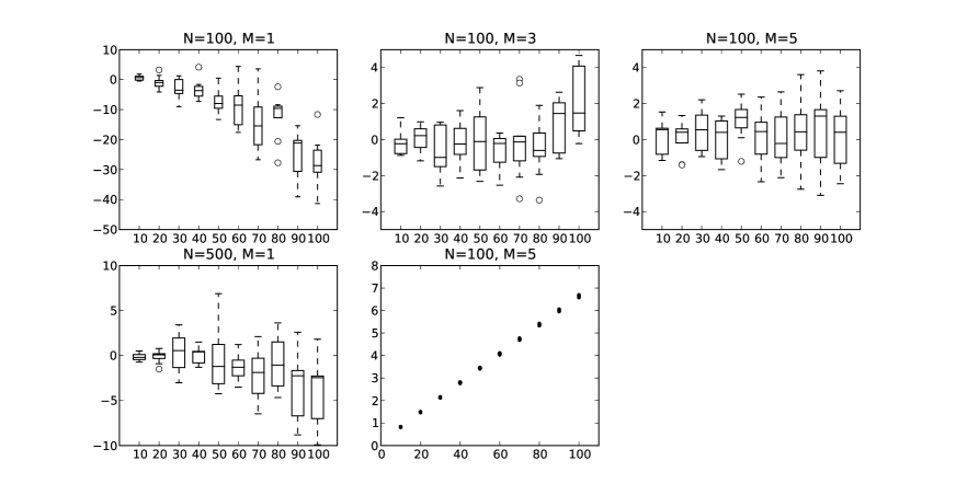
Figure 1: Decentred Gaussian example: Box-plots of the log-relative error $\log\widehat{Z}-\log Z$ versus dimension $d$ for four values of $(N,M)$, and (lower right) total number of iterations $(\times 10^{4})$ versus dimension for $(N,M)=(100,5)$

7.2 A mixture example

As in Frühwirth-Schnatter (2004), we consider the example of the posterior distribution on $(\mu,\sigma)$ associated with the normal mixture

$$y_{1},\ldots,y_{n}\sim p\mathcal{N}(0,1)+(1-p)\mathcal{N}(\mu,\sigma)\,,$$ (6)

when $p$ is known, for two compelling reasons. First, when $\sigma$ converges to $0$ and $\mu$ is equal to any of the $x_{i}$’s $(1\leq i\leq n)$, the likelihood diverges, see Fig. 2. This is a priori challenging for exploratory schemes such as nested sampling. Second, efficient Markov chain Monte Carlo strategies have been developed for mixture models (Diebolt & Robert, 1994; Richardson & Green, 1997; Celeux et al., 2000), but Bayes factors are difficult to approximate in this setting.

We simulate $n$ observations from a $\mathcal{N}(2,(3/2)^{2})$ distribution, and then compute the estimates of $Z$ introduced above for the model (6). The prior distribution is uniform on $(-2,6)\times(0\cdot 001,16)$ for $(\mu,\log\sigma^{2})$. The prior is arbitrary, but it allows for an easy implementation of nested sampling since the constrained simulation can be implemented via a random walk move.

The two-dimensional nature of the parameter space allows for a numerical integration of $L(\theta)$, based on a Riemann approximation and a grid of $800\times 500$ points in the $(-2,6)\times(0\cdot 001,16)$ square. This approach leads to a stable evaluation of $Z$ that can be taken as the reference against which we can test the various methods, since additional evaluations based on a crude Monte Carlo integration using $10^{6}$ terms and on Chib’s (1995) produced essentially the same numerical values. The Markov chain Monte Carlo algorithm implemented here is the standard completion of Diebolt & Robert (1994), but it does not suffer from the usual label switching deficiency (Jasra et al., 2005) because (6) is identifiable. As shown by the Markov chain Monte Carlo sample of size $N=10^{4}$ displayed on the left hand side of Fig. 2, the exploration of the modal region by the Markov chain Monte Carlo chain is satisfactory. This Markov chain Monte Carlo sample is used to compute the non-parametric approximations $g$ that appear in the three alternatives of §6. For the reverse importance sampling estimate $Z_{1}$, $g$ is a product of two Gaussian kernels with a bandwidth equal to half the default bandwidth of the R function density(), while, for both $Z_{2}$ and $Z_{3}$, $g$ is a product of two $t$ kernels with a bandwidth equal to twice the default Gaussian bandwidth.

We ran the nested sampling algorithm, with $N=10^{3}$, reproducing the implementation of Skilling (2006), namely using $10$ steps of a random walk in $(\mu,\log\sigma)$ constrained by the likelihood boundary. based on the contribution of the current value of $(\mu,\sigma)$ to the approximation of $Z$. The overall number of points produced by nested sampling at stopping time is on average close to $10^{4}$, which justifies using the same number of points for the Markov chain Monte Carlo algorithm. As shown on the right hand side of Fig. 2, the nested sampling sequence visits the minor modes of the likelihood surface but it ends up in the same central mode as the Markov chain Monte Carlo sequence. All points visited by nested sampling are represented without reweighting, which explains for a larger density of points outside the central modal region.

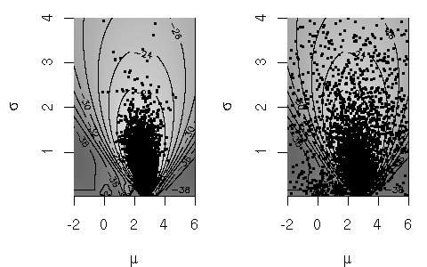
Figure 2: Mixture example: (left) Markov chain Monte Carlo sample plotted on the log-likelihood surface in the $(\mu,\sigma)$ space for $n=10$ observations from (6) (right) nested sampling sequence based on $N=10^{3}$ starting points for the same dataset

The analysis of this Monte Carlo experiment in Fig. 3 first shows that nested sampling gives approximately the same numerical value when compared with the three other approaches, exhibiting a slight upward bias, but that its variability is higher. The most reliable approach, besides the numerical and raw Monte Carlo evaluations which cannot be used in general settings, is the importance sampling solution, followed very closely by the mixture approach of §6.3. The reverse importance sampling naturally shows a slight upward bias for the smaller values of $n$ and a variability that is very close to both other alternatives, especially for larger values of $n$.

Figure 3: Mixture model: comparison of the variations of nested sampling, reverse importance sampling, importance sampling and mixture sampling, relative to a numerical approximation of $Z$ (dotted line), based on $150$ samples of size $n=10,50,100$

7.3 A probit example for nested importance sampling

To implement the nested importance sampling algorithm based on nested ellipsoids, we consider the arsenic dataset and a probit model studied in Chapter 5 of Gelman & Hill (2006). The observations are independent Bernoulli variables $y_{i}$ such that $\/ext{pr}(y_{i}=1\mid x_{i})=\Phi(x_{i}^{T}\theta)$, where $x_{i}$ is a vector of $d$ covariates, $\theta$ is a vector parameter of size $d$, and $\Phi$ denotes the standard normal distribution function. In this particular example, $d=7$; more details on the data and the covariates are available on the book’s web-page (http://www.stat.columbia.edu/~gelman/arm/examples/arsenic).

The probit model we use is model 9a in the R program available at this address: the dependent variable indicates whether or not the surveyed individual changed the well she drinks from over the past three years, and the seven covariates are an intercept, distance to the nearest safe well (in 100 metres unit), education level, log of arsenic level, and cross-effects for these three variables. We assign $\mathcal{N}_{d}(0,10^{2}I_{d})$ as our prior on $\theta$, and denote $\theta_{m}$ the posterior mode, and $\Sigma_{m}$ the inverse of minus twice the Hessian at the mode; both quantities are obtained numerically beforehand.

We run the nested ellipsoid algorithm 50 times, for $N=2$, 8, 32, 128, and for two sets of hyper-parameters corresponding to both scenarios described in §5. In the first scenario, $(\hat{\theta},\hat{\Sigma})=(\theta_{m},2\Sigma_{m})$. The bottom row of Fig. 4 compares log-errors produced by our method (left), with those of importance sampling based on the optimal Gaussian proposal, with mean $\theta_{m}$, variance $\Sigma_{m}$, and the same number of likelihood evaluations, as reported on the x-axis of the right plot. In the second scenario, $(\hat{\theta},\hat{\Sigma})=(\theta_{m},100\,I_{d})$. The top row of Fig. 4 compares log-errors produced by our method (left) with those of importance sampling, based again on the optimal proposal, and the same number of likelihood evaluations. The variance of importance sampling estimates based on a Gaussian proposal with hyper-parameters $\hat{\theta}$ and $\hat{\Sigma}=100I_{d}$ is higher by several order of magnitudes, and is not reported in the plots.

As expected, the first strategy outperforms standard importance sampling, when both methods are supplied with the same information (mode, Hessian), and the second strategy still does reasonably well compared to importance sampling based on the optimal Gaussian proposal, although only provided with the mode. Results are sufficiently precise that one can afford to compute the evidence for the $2^{7}$ possible models: the most likely model, with posterior probability $0.81$, includes the intercept, the three variables mentioned above, distance, arsenic, education, and one cross-effect between distance and education level, and the second most likely model, with posterior probability $0.18$, is the same model but without the cross-effect.

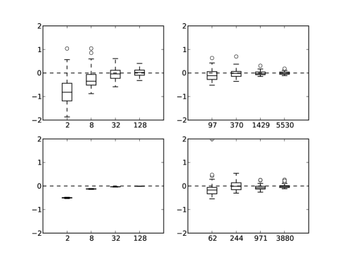
Figure 4: Probit example: Box-plots of (left column) log-errors of nested importance sampling estimates, for $N=2,$ $8,$ $32$, $128$, compared with the log-error of importance sampling estimates (right column) based on the optimal Gaussian proposal, and the same number of likelihood evaluations. Those are reported on the x axis of the right column plots. The bottom row corresponds to the first strategy, based on both mode and Hessian, while the top row corresponds to the second strategy, based on mode only.

8 Discussion

Nested sampling is thus a valid addition to the Monte Carlo toolbox, with convergence rate $\text{O}(N^{-1/2})$, and computational cost $O(d^{3})$, where $d$ is the dimension of the problem. which enjoys good performances in some applications, for example when the posterior is approximately Gaussian, but which may require more iterations to achieve the same precision in certain situations. Therefore, further work on the formal and practical assessments of nested sampling convergence would be welcome. For one thing, the convergence properties of Markov chain Monte Carlo-based nested sampling are unknown and technically challenging. Methodologically, efforts are required to design efficient Markov chain Monte Carlo moves with respect to the constrained prior. In that and other respects, nested importance sampling may constitute a useful extension. Ultimately, our comparison between nested sampling and alternatives should be extended to more diverse examples, in order to get a clearer idea of when nested sampling should be the method of choice and when it should not. For instance, Murray et al. (2006) reports that nested sampling strongly outperforms annealed importance sampling (Neal, 2001) for Potts models. All the programs implemented for this paper are available from the authors.

Appendix 1

Proof of Lemma 2.1

It is sufficient to prove this result for functions $\widetilde{f}$ that are real-valued, positive and increasing. First, the extension to vector-valued functions is trivial, so $\widetilde{f}$ is assumed to be real-valued from now on. Second, the class of functions that satisfy property (4) is clearly stable through addition. Since $\widetilde{f}$ is absolutely continuous, there exist functions $f^{+}$ and $f^{-}$, such that $f^{+}$ is increasing, $f^{-}$ is decreasing, and $\widetilde{f}=f^{+}+f^{-}$, so we can restrict our attention to increasing functions. Third, absolute continuity implies bounded variation, so it always possible to add an arbitrary constant to $\widetilde{f}$ to transform it into a positive function.

Let $\psi:l\rightarrow l\widetilde{f}(l)$, which is a positive, increasing function and denote its inverse by $\psi^{-1}$. One has:

$$E^{\pi}[\psi\{L(\theta)\}]=\int_{0}^{+\infty}\mathrm{pr}[\psi\{L(\theta)\}>l]\,\text{d}l=\int_{0}^{+\infty}\varphi^{-1}\{\psi^{-1}(l)\}\,\text{d}l=\int_{0}^{1}\psi\{\varphi(x)\}\,\text{d}x\,,$$

which concludes the proof.

Appendix 2

Proof of Theorem 1

Let $t_{i}=x_{i+1}^{\star}/x_{i}^{\star}$, for $i=0,1,\ldots$ As mentioned by Skilling (2006), the $t_{i}$’s are independent beta$(N,1)$ variates. Thus, $u_{i}=t_{i}^{N}$ defines a sequence of independent uniform $[0,1]$ variates. A Taylor expansion of $\eta_{N}$ gives:

$$\eta_{N} = \sum_{i=1}^{\left\lceil cN\right\rceil}(x_{i-1}-x_{i})\left\{\varphi(x_{i}^{\star})-\varphi(x_{i})\right\}$$

$$= \sum_{i=1}^{\left\lceil cN\right\rceil}(x_{i-1}-x_{i})\left\{\psi^{\prime}(-\log x_{i})\left(\log x_{i}-\log x_{i}^{\star}\right)+O\left(\log x_{i}-\log x_{i}^{\star}\right)^{2}\right\}$$

where $c=-\log\varepsilon$, and $\psi(y)=\varphi(e^{-y})$. Furthermore,

$$S_{i}=N\left(\log x_{i}-\log x_{i}^{\star}\right)=\sum_{k=0}^{i-1}(-1-\log u_{k})$$

is a sum of independent, standard variables, as $E(\log u_{i})=-1$ and $\text{var}(\log u_{i})=1$. Thus, $\left(\log x_{i}-\log x_{i}^{\star}\right)=\text{O}_{P}(N^{-1/2})$, where the implicit constant in $\text{O}_{P}(N^{-1/2})$ does not depend on $i$, and

$$N^{1/2}\eta_{N} = N^{-1/2}\sum_{i=1}^{\lceil cN\rceil}(e^{-(i-1)/N}-e^{-i/N})S_{i}\left\{\psi^{\prime}(\frac{i}{N})+O_{P}(N^{-1/2})\right\}$$

$$= c^{1/2}\sum_{i=1}^{\lceil cN\rceil}\int_{(i-1)/N}^{i/N}e^{-t}\psi^{\prime}(t)B_{N}(\frac{t}{c})\ \text{d}t\left\{1+O_{P}(N^{-1/2})\right\}\,,$$

since $\psi^{\prime}(t)=\psi^{\prime}(i/N)+\text{O}(N^{-1})$ for $t\in[(i-1)/N,i/N]$, where, again, the implicit constant in $\text{O}(N^{-1})$ can be the same for all $i$, as $\psi^{\prime\prime}$ is bounded, and provided $B_{N}(t)$ is defined as $B_{N}(t)=(cN)^{-1/2}S_{\left\lceil cNt\right\rceil}$for $t\in[0,1]$. According to Donsker’s theorem (Kallenberg, 2002, p.275), $B_{N}$ converges to a Brownian motion $B$ on $[0,1]$, in the sense that $f(B_{N})$ converges in distribution to $f(B)$ for any measurable and a.s. continuous function $f$. Thus

$$N^{1/2}\eta_{N}=c^{1/2}\int_{0}^{\left\lceil cN\right\rceil/N}e^{-t}\psi^{\prime}(t)B_{N}(\frac{t}{c})\ \text{d}t+O_{P}(N^{-1/2})$$

converges in distribution to

$$c^{1/2}\int_{0}^{c}e^{-t}\psi^{\prime}(t)B(\frac{t}{c})\,\text{d}t\,,$$

which has the same distribution as the following zero-mean Gaussian variate:

$$\int_{0}^{c}e^{-t}\psi^{\prime}(t)B(t)\,\text{d}t=\int_{\varepsilon}^{1}s\varphi^{\prime}(s)B(-\log s)\,\text{d}s.$$

Appendix 3

Proof of Lemma 4.1

For the sake of clarity, we make dependencies on $d$ explicit in this section, including $\varphi_{d}$ for $\varphi$, $\varepsilon_{d}$ for $\varepsilon$, and so on. We will use repeatedly the facts that $\varphi$ is nonincreasing and that $\varphi^{\prime}$ is nonnegative. One has:

$$-\int_{s,t\in[\varepsilon_{d},1]}s\varphi_{d}^{\prime}(s)t\varphi_{d}^{\prime}(t)\log(s\vee t)\,\text{d}t\leq-\log\varepsilon_{d}\left\{\int_{\varepsilon_{d}}^{1}s\varphi_{d}^{\prime}(s)\,\text{d}s\right\}^{2}\leq d\log(2^{1/2}/\tau)$$

for $d\geq 1$, since $-\int_{\varepsilon_{d}}^{1}s\varphi_{d}^{\prime}(s)\,\text{d}s\leq-\int_{0}^{1}s\varphi_{d}^{\prime}(s)\,\text{d}s=1$. This gives the first result.

Let $s_{d}=\varphi_{d}^{-1}(\alpha^{d})$, for $0<\alpha<1$; $s_{d}$ is the probability that

$$(4\pi/d){\sum_{i=1}^{d}\theta_{i}^{2}}-1\leq-2\log(\alpha)+\log(2)-1$$

assuming that the $\theta_{i}$’s are independent $\mathcal{N}(0,1/4\pi)$ variates. The left-hand side is an empirical average of independent and identically distributed zero-mean variables. We take $\alpha$ so that the right-hand side is negative, which implies $\alpha>2^{1/2}\exp(-1/2)$. Using large deviations (Kallenberg, 2002, Chapter 27), one has $-\log(s_{d})/d\rightarrow\gamma>0$ as $d\rightarrow+\infty,$ and

$$\frac{1}{d}V_{d} = -\frac{1}{d}\int_{s,t\in[\varepsilon_{d},1]}s\varphi_{d}^{\prime}(s)t\varphi_{d}^{\prime}(t)\log(s\vee t)\,\text{d}s\text{d}t$$

$$\geq \left\{\frac{-\log s_{d}}{d}\right)\left(\int_{\varepsilon_{d}}^{s_{d}}s\varphi_{d}^{\prime}(s)\,\text{d}s\right\}^{2}$$

$$\geq \left(\frac{-\log s_{d}}{d}\right)\left\{\int_{\varepsilon_{d}}^{s_{d}}\varphi_{d}(s)\,\text{d}s+\varepsilon_{d}\varphi_{d}(\varepsilon_{d})-s_{d}\varphi_{d}(s_{d})\right\}^{2}$$

$$\geq \left(\frac{-\log s_{d}}{d}\right)\left\{1-\int_{0}^{\varepsilon_{d}}\varphi_{d}(s)\,\text{d}s-\int_{s_{d}}^{1}\varphi_{d}(s)\,\text{d}s+\varepsilon_{d}\varphi_{d}(\varepsilon_{d})-s_{d}\varphi_{d}(s_{d})\right\}^{2}.$$

As $d\rightarrow+\infty$, $-\log(s_{d})/d\rightarrow\gamma$, $s_{d}\rightarrow 0$, $\varphi_{d}(s_{d})=\alpha^{d}\rightarrow 0$, $\int_{s_{d}}^{1}\varphi_{d}(s)\,\text{d}s\leq\varphi_{d}(s_{d})(1-s_{d})\rightarrow 0$, and

$$0\leq\int_{0}^{\varepsilon_{d}}\varphi_{d}(s)\,\text{d}s-\varepsilon_{d}\varphi_{d}(\varepsilon_{d})\leq\varepsilon_{d}\{\varphi_{d}(0)-\varphi_{d}(\varepsilon_{d})\}\leq\tau<1,$$

by the definition of $\varepsilon_{d}$, and the squared factor is in the limit greater than or equal to $(1-\tau)^{2}$.

References

- Bartolucci et al. (2006) Bartolucci, F., Scaccia, L. & Mira, A. (2006). Efficient Bayes factor estimation from the reversible jump output. Biometrika 93, 41–52.
- Brockwell & Davis (1996) Brockwell, P. & Davis, P. (1996). Introduction to Time Series and Forecasting. Springer Texts in Statistics. Springer-Verlag, New York.
- Celeux et al. (2000) Celeux, G., Hurn, M. & Robert, C. (2000). Computational and inferential difficulties with mixtures posterior distribution. J. Am. Statist. Assoc. 95(3), 957–979.
- Chen & Shao (1997) Chen, M. & Shao, Q. (1997). On Monte Carlo methods for estimating ratios of normalizing constants. Ann. Statist. 25, 1563–1594.
- Chen et al. (2000) Chen, M., Shao, Q. & Ibrahim, J. (2000). Monte Carlo Methods in Bayesian Computation. Springer-Verlag, New York.
- Chib (1995) Chib, S. (1995). Marginal likelihood from the Gibbs output. J. Am. Statist. Assoc. 90, 1313–1321.
- Diebolt & Robert (1994) Diebolt, J. & Robert, C. (1994). Estimation of finite mixture distributions by Bayesian sampling. J. R. Statist. Soc. A 56, 363–375.
- Evans (2007) Evans, M. (2007). Discussion of nested sampling for Bayesiancomputations by John Skilling. In Bayesian Statistics 8, J. Bernardo, M. Bayarri, J. Berger, A. David, D. Heckerman, A. Smith & M. West, eds. Oxford University Press, pp. 491–524.
- Frühwirth-Schnatter (2004) Frühwirth-Schnatter, S. (2004). Estimating marginal likelihoods for mixture and Markov switching models using bridge sampling techniques. The Econometrics Journal 7, 143–167.
- Gelfand & Dey (1994) Gelfand, A. & Dey, D. (1994). Bayesian model choice: asymptotics and exact calculations. J. R. Statist. Soc. A 56, 501–514.
- Gelman & Hill (2006) Gelman, A. & Hill, J. (2006). Data Analysis Using Regression and Multilevel/Hierarchical Models. Cambridge, UK: Cambridge University Press.
- Green (1995) Green, P. (1995). Reversible jump MCMC computation and Bayesian model determination. Biometrika 82, 711–732.
- Han & Carlin (2001) Han, C. & Carlin, B. (2001). MCMC methods for computing Bayes factors: a comparative review. J. Am. Statist. Assoc. 96, 1122–1132.
- Hesterberg (1998) Hesterberg, T. (1998). Weighted average importance sampling and defensive mixture distributions. Technometrics 37, 185–194.
- Jasra et al. (2005) Jasra, A., Holmes, C. & Stephens, D. (2005). Markov Chain Monte Carlo methods and the label switching problem in Bayesian mixture modeling. Statist. Sci. 20, 50–67.
- Jeffreys (1939) Jeffreys, H. (1939). Theory of Probability. Oxford: The Clarendon Press, 1st ed.
- Kallenberg (2002) Kallenberg, O. (2002). Foundations of Modern Probability. Springer-Verlag, New York.
- Louis (1982) Louis, T. (1982). Finding the observed information matrix when using the EM algorithm. J. R. Statist. Soc. A 44, 226–233.
- MacLachlan & Krishnan (1997) MacLachlan, G. & Krishnan, T. (1997). The EM Algorithm and Extensions. New York: John Wiley.
- Meng & Schilling (2002) Meng, X. & Schilling, S. (2002). Warp bridge sampling. J. Comput. Graph. Statist. 11, 552–586.
- Meng & Wong (1996) Meng, X. & Wong, W. (1996). Simulating ratios of normalizing constants via a simple identity: a theoretical exploration. Statist. Sinica 6, 831–860.
- Mukherjee et al. (2006) Mukherjee, P., Parkinson, D. & Liddle, A. (2006). A Nested Sampling Algorithm for Cosmological Model Selection. The Astrophysical Journal 638, L51–L54.
- Murray et al. (2006) Murray, I., MacKay, D. J., Ghahramani, Z. & Skilling, J. (2006). Nested sampling for Potts models. In Advances in Neural Information Processing Systems 18, Y. Weiss, B. Schölkopf & J. Platt, eds. Cambridge, MA: MIT Press.
- Neal (2001) Neal, R. (2001). Annealed importance sampling. Stat. Comput. 11, 125–139.
- Richardson & Green (1997) Richardson, S. & Green, P. (1997). On Bayesian analysis of mixtures with an unknown number of components (with discussion). J. R. Statist. Soc. A 59, 731–792.
- Robert (2001) Robert, C. (2001). The Bayesian Choice. Springer-Verlag, New York, 2nd ed.
- Roberts & Rosenthal (1999) Roberts, G. & Rosenthal, J. (1999). Convergence of slice sampler Markov chains. J. R. Statist. Soc. A 61, 643–660.
- Rydén (1994) Rydén, T. (1994). Parameter estimation for Markov modulated Poisson processes. Stochastic Models 10, 795–829.
- Shaw et al. (2007) Shaw, J., Bridges, M. & Hobson, M. (2007). Efficient Bayesian inference for multimodal problems in cosmology. Monthly Not. R. Astrono. Soc. 378, 1365–1370.
- Skilling (2006) Skilling, J. (2006). Nested sampling for general Bayesian computation. Bayesian Analysis 1(4), 833–860.
- Spiegelhalter et al. (2002) Spiegelhalter, D. J., Best, N. G., Carlin, B. P. & van der Linde, A. (2002). Bayesian measures of model complexity and fit (with discussion). J. R. Statist. Soc. A 64, 583–639.
- Vegetti & Koopmans (2009) Vegetti, S. & Koopmans, L. V. E. (2009). Bayesian strong gravitational-lens modelling on adaptive grids: objective detection of mass substructure in galaxies. Monthly Not. R. Astrono. Soc. 392, 945–963.