Towards a Real-Time Data Driven Wildland Fire Model

Abstract

A wildland fire model based on semi-empirical relations for the spread rate of a surface fire and post-frontal heat release is coupled with the Weather Research and Forecasting atmospheric model (WRF). The propagation of the fire front is implemented by a level set method. Data is assimilated by a morphing ensemble Kalman filter, which provides amplitude as well as position corrections. Thermal images of a fire will provide the observations and will be compared to a synthetic image from the model state.

1. Introduction

In this paper, we review the current state of a project in wildland fire simulation based on real-time sensor monitoring. The model will be driven by real-time data and run on remote supercomputers. The state of the model will be adjusted from real-time airborne imagery as well as ground sensor data. We have also used a regularization approach to EnKF for wildfire [7] with a fire model by reaction-diffusion-convection partial differential equations [12]. See [10] for an earlier picture of this project.

2. Coupled fire-atmosphere model

This section is based on [11], with some new developments. Our current code implements the mathematical ideas from [3] in a simplified contemporary numerical framework in that the fire propagation, originally done by a custom ad hoc tracer code, is now done using a simpler level set method, and the fire model is now coupled with the Weather Research and Forecasting model (WRF, www.wrf-model.org), a community supported numerical weather prediction code. This adds capabilities to the codes used in previous work such as theoretical experiments of [3] and [4], where it was used in reanalysis of a real fire. Specifically, it allows taking advantage of the WRF architecture, which provides a natural parallelization of both the fire and the atmospheric code in shared as well as distributed memory and support for data assimilation.

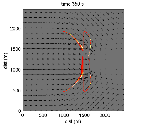
Figure 1: Coupled fire-atmosphere simulation. Fire propagates from two line ignitions and one circle ignition, which are in the process of merging. The arrows are horizontal wind at ground level. False color is fire heat flux. The fire front on the right has irregular shape and is slowed down because of air being pulled up by the heat created by the fire. This kind of fire behavior cannot be modeled by empirical spread models alone.

2.1. Fire spread model

We use a semi-empirical fire propagation model [3, 13] to represent a fire spreading on the surface. Given wind speed $\overrightarrow{v}$ and terrain height $z$, the model postulates that the fireline evolves with the spread rate $S$ in the normal direction to the fireline $\overrightarrow{n}$ given by

$$S=R_{0}+a\left(\overrightarrow{v}\cdot\overrightarrow{n}\right)^{b}+d\nabla z\cdot\overrightarrow{n},$$

where $R_{0}$, $a$, $b,$ and $d$ are fuel coefficients determined from laboratory experiments. In addition, the spread rate is cut off to satisfy $0\leq S\leq S_{\max}$, where $S_{\max}$ depends on the fuel. Based on laboratory experiments, the model further assumes that after ignition the fuel amount decreases as an exponential function of time, the characteristic time scale depending on the fuel type (rapid mass loss in grass, slow mass loss in larger fuel particles). The output of the model is the sensible and the latent heat fluxes (temperature and water vapor) from the fire to the atmosphere, taken to be proportional to the amount of fuel burned.

2.2. Propagation by level set method

In the level set method, the burning area at time $t$ is represented as $\left\{\left(x,y\right):\psi\left(x,y,t\right)<0\right\}$, where $\psi$ is the level set function. The fireline at time $t$ is the level set $\left\{\left(x,y\right):\psi\left(x,y,t\right)=0\right\}$. The normal to the fireline can be computed from the level set function as $\overrightarrow{n}=\nabla\psi/\left\|\nabla\psi\right\|$. The level set function satisfies the differential equation ${\partial\psi}/{\partial t}+S\left\|\nabla\psi\right\|=0$, which we solve numerically by the Heun’s method (i.e., Runge-Kutta method of order 2) using approximation of $\nabla\psi$ from upwinded approximation of $\nabla\psi$ by Godunov’s method: each partial derivative is approximated by the left difference if both the left and the central differences are nonnegative, by the right difference if both the right and the central differences are nonpositive, and taken as zero otherwise. The reason for using Heun’s method is not accuracy but conservation: the explicit Euler method systematically overestimates $\psi$ and thus slows down fire propagation or even stops it altogether while Heun’s method behaves reasonably well. The level set function is initialized to the signed distance from the fireline.

2.3. Coupling with weather

The fire model takes as input the horizontal wind velocity components and outputs the heat fluxes. The finest atmospheric mesh interfaces with the fire. However, WRF meshes cannot be nested vertically, so even the finest mesh still goes vertically over the whole atmosphere. We have used time step $0.5$s with the $60$m finest atmospheric mesh step and $6$m fire mesh step, which satisfied the CFL stability conditions in the fire and in the atmosphere.

The heat flux from the fire model cannot be applied directly as a boundary condition on the derivatives of the corresponding physical field (air temperature or water vapor contents) because WRF does not support flux boundary conditions. Instead, the flux is inserted by modifying the temperature and water vapor concentration over a depth of many cells, with exponential decay away from the boundary.

3. Data assimilation

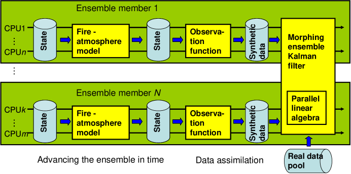
Figure 2: Parallel implementation of one assimilation cycle. Ensemble members are advanced in time and the observation function evaluated for each ensemble member independently on a subset of processors. The morphing EnKF adjusts the member states by comparing the synthetic data with real data and balances the uncertainty in the data, which is given as error bound, with the uncertainty in the simulation, computed from the spread of the whole ensemble. The morphing EnKF runs on all processors. The ensemble of model states is maintained in disk files. The observation function takes as input the disk files and delivers synthetic data also in disk files. The EnKF inputs the synthetic data and the real data, and modifies the files with the ensemble states. The model, the observation function, and the EnKF are in separate executables.

The overall scheme is in Fig. 2. We are using the ensemble Kalman filter (EnKF) [6] for data assimilation. We currently know how to work with data from airborne/space images and land-based sensors, though work remains on making all the connections described. In the rest of this section we describe how to treat various kinds of data (Sec. 3.1.), how can synthetic image data for the fire be obtained from the system state (Sec. 3.2.), and how is are the model states adjusted by in response the the data (Sec. 3.3.).

3.1. Data sources

To date, our efforts have been to get data from a variety of sources (e.g., weather stations, aerial images, etc.) and to compare it [2] to data from the fire-atmosphere code [3]. A state vector is handed to the observation function routines and the vector is modified and returned. The state is transferred using disk files. Individual subvectors corresponding to the most common variables are extracted or replaced in the files. A software layer exists in order to hide both the fire code and the data transfer method so that the code is not dependent on a particular fire-atmosphere code.

Consider an example of a weather station that reports its location, a timestamp, temperature, wind velocity, and humidity. The atmosphere code has multiple nested grids. For a given grid, we have to determine in which cell the weather station is located, which is done using linear interpolation of the location. The data is is determined at relevant grid points using biquadratic interpolation. We compare the computed results with the weather station data. We determine if a fireline is in the cell (or neighboring ones) with the weather station temperature to see if there really is a fire in the cell. Currently, the state vector is updated for the temperature and returned for further processing. In future, this will be replaced by the output of synthetic data in disk files for the data assimilation, as in Fig. 2.

3.2. Synthetic scene generation

The purpose of synthetic scene generation [15] is to use the model state to produce an image just like one from the infrared camera, so that it can be compared to the actual data in the data assimilation. The synthetic scene generation depends on the propagation model, parameters such as velocity of the fire movement, as well as its output (the heat flux), and the input (the wind speed). The use of the parameters from the model allows us to estimate the 3D flame structure, which provides an effective geometry for simulating radiance from the fire scene. Given the 3D flame structure, we assume we can adequately estimate the infrared scene radiance by including three aspects of radiated energy. These are radiation from the hot ground under the fire front and the cooling of the ground after the fire front passes, which accounts for the heating and cooling of the 2D surface, the direct radiation to the sensor from the 3D flame, which accounts for the intense radiation from the flame itself, and the radiation from the 3D flame that is reflected from the nearby ground. This reflected radiation is most important in the near and mid-wave infrared spectrum. Reflected long-wave radiation is much less important because of the high emissivity (low reflectivity) of burn scar in the long-wave infrared portion of the spectrum [9].

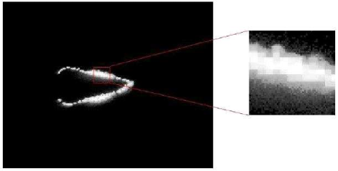
Figure 3: Synthetic fire scene. A DIRSIG rendering of the midwave (3-5 micrometers) infrared radiation from a modeled grassfire. The scene is rendered as it would be observed with RIT’s WASP airborne infrared camera system flying about 3000 m above ground. The zoomed area shows the effect of the hot ground and voxelized flame structure in the central blocky pixels and the lighter gray fading away at the edges is the reflected radiation from the 3D flame. From [15].

The 2D fire front and cooling are estimated with a double exponential. The time constants are 75 seconds and 250 seconds and the peak temperature at the fire front is constrained to 1075K. The position of the fire front is determined from the propagation model described above. The 3D flame structure is estimated by using the heat release rate and experimental estimates of flame width and length and the flame is tilted based on wind speed. This 3D structure is represented by a 3D grid of voxels.

The 2D ground temperatures and the 3D voxels representing the flame are inputs to a ray tracing code for determining the radiance from those sources as they would be viewed by an airborne remote sensing system. The ray tracing code used is the Digital Imaging and Remote Sensing Image Generation Model (DIRSIG). The Digital Imaging and Remote Sensing Image Generation (DIRSIG) model is a first principles based synthetic image generation model developed by the Digital Imaging and Remote Sensing Laboratory at RIT [5, 14]. The model can produce multi- or hyper-spectral imagery from the visible through the thermal infrared region of the electromagnetic spectrum. Radiance reflected from the ground and the effects of the atmosphere are include in the radiance calculation. The resulting synthetic radiance image (Fig. 3) was validated by calculation of the fire radiated energy and comparing those results to published values derived from satellite remote sensing data over wildland fires [16]. We are continuing to work on synthetic image generation with the goal of replacing the computationally intensive, but accurate, ray tracing method with a simpler method of calculating the fire radiance based upon the radiance estimations that are inherent in the fire propagation model.

3.3. Morphing ensemble Kalman filter

This section again follows [11]. The state of the model consists of the level set function $\psi$ and the ignition time $t_{i}$, both given as arrays of values associated with grid nodes. These grid arrays can be modified by data assimilation methods with relative ease, unlike the tracers in [3]. Data assimilation [8] maintains an approximation of the probability distribution of the state. In each analysis cycle, the probability distribution of the state is advanced in time and then updated from the data likelihood using the Bayes theorem. EnKF represents the probability distribution of the state by an ensemble and it uses the model only as a black box, without any additional coding required. After advancing the ensemble in time, the EnKF replaces the ensemble by its linear combinations with the coefficients obtained by solving a least squares problem to balance the change in the state and the difference from the data.

However, the EnKF applied directly to the model fields does not work well when the data indicate a fire in a different location than in the state, because such data have infinitesimally small likelihood and the span of the ensemble does contain a state consistent with the data. Therefore, we adjust also the simulation state by changing the position of the fire rather than an additive correction alone, by borrowing the techniques of registration and morphing from image processing. Essentially, we replace the linear combinations of states in the EnKF by intermediate states obtained by morphing, which leads to the morphing EnKF method [1].

Given two functions $u_{0}$, $u$, representing the same physical field, such as the temperature, or the level set function, from two states of the coupled model, registration can be described as finding a mapping $T$ of the spatial domain so that $u\approx u_{0}\circ\left(I+T\right)$, where $\circ$ denotes the composition of mappings and $I$ is the identity mapping. The field $u$ and the mapping $T$ are given by their values on a grid. To find the registration mapping  $T$ automatically, we solve approximately an optimization problem of the form

$$\left\|u-u_{0}\circ\left(I+T\right)\right\|+\left\|T\right\|+\left\|\nabla T\right\|\rightarrow\min.$$

We then construct intermediate functions $u_{\lambda}$ between $u_{0}$ and $u_{1}$ by [1]

$$u_{\lambda}=\left(u+\lambda r\right)\circ\left(I+\lambda T\right),\quad 0\leq\lambda\leq 1,$$ (1)

where $r=u\circ\left(I+T\right)^{-1}-u_{0}$. The morphing EnKF works by transforming the ensemble member into extended states of the form $\left[r,T\right]$, which are input into the EnKF. The result is then converted back by (1). See Fig. 4 for an illustrative result.

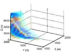
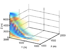
(a)	(b)
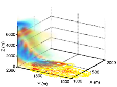
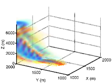
(c)	(d)

Figure 4: The morphing EnKF applied to the fireline propagation model coupled with WRF. False color and contour on the horizontal plane is the fire heat flux. The volume shading is the vorticity of the atmosphere. The reference solution (a) is the simulated data. The initial ensemble was created by a random perturbation of the comparison solution (b), with the fire ignited at an intentionally incorrect location. The standard ENKF (c) and the morphing EnKF (d) were applied after 15 minutes. The ensembles have 25 members each, with the heat fluxes shown superimposed. The standard EnKF ensembles diverges from the data, while the morphing EnKF ensemble keeps closer to the data. Reproduced from [11].

4. Acknowledgement

This work was supported by NSF grants CNS-0325314, CNS-0324910, CNS-0324989, CNS-0324876, CNS-0540178, CNS-0719641, CNS-0719626, CNS-0720454, DMS-0623983, EIA-0219627, and OISE-0405349.

References

- [1] J. D. Beezley and J. Mandel. Morphing ensemble Kalman filters. Tellus, 60A:131–140, 2008.
- [2] S. Chakraborty. Data assimilation and visualization for ensemble wildland fire models. Master’s thesis, University of Kentucky, Coputer Science, Lexington, KY, 2008.
- [3] T. L. Clark, J. Coen, and D. Latham. Description of a coupled atmosphere-fire model. Intl. J. Wildland Fire, 13:49–64, 2004.
- [4] J. L. Coen. Simulation of the Big Elk Fire using coupled atmosphere-fire modeling. Intl. J. Wildland Fire, 14(1):49–59, 2005.
- [5] DIRSIG users manual. Digital Imaging and Remote Sensing Laboratory. Rochester Institute of Technology. http://www.dirsig.org/docs/manual-2006-11.pdf, 2006.
- [6] G. Evensen. The ensemble Kalman filter: Theoretical formulation and practical implementation. Ocean Dynamics, 53:343–367, 2003.
- [7] C. J. Johns and J. Mandel. A two-stage ensemble Kalman filter for smooth data assimilation. Environmental and Ecological Statistics, in print, 2008.
- [8] E. Kalnay. Atmospheric Modeling, Data Assimilation and Predictability. Cambridge University Press, 2003.
- [9] R. Kremens, J. Faulring, and C. C. Hardy. Measurement of the time-temperature and emissivity history of the burn scar for remote sensing applications. Paper J1G.5, Proceedings of the 2nd Fire Ecology Congress, Orlando FL, American Meteorological Society, 2003.
- [10] J. Mandel, J. D. Beezley, L. S. Bennethum, S. Chakraborty, J. L. Coen, C. C. Douglas, J. Hatcher, M. Kim, and A. Vodacek. A dynamic data driven wildland fire model. Lecture Notes in Computer Science, 4487:1042–1049, 2007.
- [11] J. Mandel, J. D. Beezley, J. L. Coen, and M. Kim. Data assimilation for wildland fires: Ensemble Kalman filters in coupled atmosphere-surface models. arXiv:0712.3965, 2007.
- [12] J. Mandel, L. S. Bennethum, J. D. Beezley, J. L. Coen, C. C. Douglas, L. P. Franca, M. Kim, and A. Vodacek. A wildfire model with data assimilation. arXiv:0709.0086, 2006.
- [13] R. C. Rothermel. A mathematical model for predicting fire spread in wildland fires. USDA Forest Service Research Paper INT-115, 1972.
- [14] J. Schott, S. D. Brown, R. V. Raqueño, H. N. Gross, and G. Robinson. An advanced synthetic image generation model and its application to multi/hyperspectral algorithm development. Canadian Journal of Remote Sensing, 25:99–111, 1999.
- [15] Z. Wang. Modeling Wildland Fire Radiance in Synthetic Remote Sensing Scenes. PhD thesis, Rochester Institute of Technology, Center for Imaging Science, 2008.
- [16] M. J. Wooster, B. Zhukov, and D. Oertel. Fire radiative energy for quantitative study of biomass burning: derivation from the BIRD experimental satellite and comparison to MODIS fire products. Remote Sensing of Environment, 86:83–107, 2003.