The Adiabatic Theorem in the Presence of Noise

Abstract

We provide rigorous bounds for the error of the adiabatic approximation of quantum mechanics under four sources of experimental error: perturbations in the initial condition, systematic time-dependent perturbations in the Hamiltonian, coupling to low-energy quantum systems, and decoherent time-dependent perturbations in the Hamiltonian. For decoherent perturbations, we find both upper and lower bounds on the evolution time to guarantee the adiabatic approximation performs within a prescribed tolerance. Our new results include explicit definitions of constants, and we apply them to the spin-1/2 particle in a rotating magnetic field, and to the superconducting flux qubit. We compare the theoretical bounds on the superconducting flux qubit to simulation results.

1 Introduction

Adiabatic quantum computation [7] (AQC) is a model of quantum computation equivalent to the standard model [1]. A physical system is slowly evolved from the ground state of a simple system, to one whose ground state encodes the solution to the difficult problem. By a physical principle known as the adiabatic approximation, if the evolution is done sufficiently slowly, and the minimum energy gap separating the ground state from higher states is sufficiently large, then the final state of the system should be the state encoding the solution to some problem.

The biggest hurdles facing many potential implementations of a quantum computer are the errors due to interaction of the qubits with the environment. However, the effects of such errors are different in AQC than in standard quantum computing. AQC is robust against dephasing in the ground state, for instance [5], and some have suggested that noise in some regimes might actually assist adiabatic quantum computation [9].

The physical principle underlying AQC is established by the Adiabatic Theorem (AT). The AT bounds the run-time of the algorithm using the minimum energy gap of the system during the evolution. The AT itself has been recently subject to controversy [14, 23, 24], and cannot be applied directly to systems with noise or decoherence. There have been some numerical studies of AQC in the presence of noise [5, 9], and an analytic random-matrix study [17]. Several recent studies have focused on the adiabatic approximation in open quantum systems using the density operator formalism [19, 21, 28, 8, 22]. However, it is difficult to derive rigorous bounds with this approach because the dynamics involve a non-Hermitian operator without a complete set of orthonormal eigenstates.

The subject of this work is the study of the adiabatic theorem in the presence of noise, perturbations, and decoherence. We consider several ways to extend the application of the theorem. Our statements, derived from Avron’s version of the theorem [2], include explicit definitions of constants, so that we may apply them on examples.

Experimental error for quantum computing experiments can be conveniently divided into three categories [25]:

1. Coherent errors, due to a systematic implementation error such as miscalibration in a magnetic field generator.

2. Incoherent errors, due to deterministic qubit-level differences in the evolution such as those caused by manufacturing defects.

3. Decoherent errors, which are are random qubit-level errors due to coupling with the environment.

In Section 2, we prove several extensions of the adiabatic theorem to handle these different types of error. For coherent errors, we provide a theorem for perturbations in the initial state of the system, and a theorem for systematic time-dependent perturbations in the Hamiltonian. In the case of decoherent errors, we provide two new theorems, one for open quantum systems and one for noise modeled as a time-dependent perturbation in the Hamiltonian.

In Section 3, we apply the new theorems to the spin-1/2 particle in a rotating magnetic field, a standard example for controversy regarding the Adiabatic Theorem [4, 23, 27, 13]. We show our theorems make correct predictions about the error of the adiabatic approximation.

Finally, in Section 4 we apply the new theorems to the superconducting flux qubit [15], which has been proposed for adiabatic quantum computation [11]. We use our theorems to determine a range of evolution times where the adiabatic approximation is guaranteed to perform well for a typical set of physical parameters and an apparently reasonable physical noise source. This provides the experimentalist with analytic tools for determining parameters to guarantee the adiabatic approximation works well, without the need to perform numerical simulations.

2 Adiabatic Theorems for Noisy Hamiltonian Evolutions

We begin with a Hamiltonian evolution $\mathcal{H}(s)$ parameterized by $s\in[0,1]$. If we define $\tau$ to be the total evolution time, then the Hamiltonian at time $t$ is $\mathcal{H}(t/\tau)$. Thus, as $\tau$ grows, $\mathcal{H}(s)$ describes a slower evolution. Assume $\mathcal{H}(s)$ has countable eigenstates $\{|\psi_{j}(s)\rangle\}$ and eigenvalues $\lambda_{0}(s)\leq\lambda_{1}(s)...$, and consider the subspace

$$\Psi(s)={\rm Span}\left\{|\psi_{m}(s)\rangle,...,|\psi_{n}(s)\rangle\right\}\;,$$ (1)

for some $0\leq m\leq n$. Then the adiabatic approximation states that if the state of the system is contained in $\Psi(0)$ at $t=0$, then at time $t=s/\tau$ the state is contained in $\Psi(s)$. Notice that while the ground state $|\psi_{0}(s)\rangle$ may be important for physical reasons, the definition above allows consideration of a more general set of states.

It is convenient to define an operator that computes the error of the adiabatic approximation for a Hamiltonian evolution. We will need the projection operator $P(s)$ that projects a state onto $\Psi(s)$. We will also need the unitary evolution operator $U(s)$, that is the solution to Schrödinger’s equation in the form

$$\dot{U}(s)=-i\tau\mathcal{H}(s)U(s)\;.$$ (2)

To compute the error of the adiabatic approximation, we apply $P(0)$ to obtain the component of the initial state contained in $\Psi(0)$, evolve it forward in time by applying $U(s)$, and then apply $I-P(s)$ to compute the component of the state outside $\Psi(s)$. For convenience, we define $Q(s)=I-P(s)$, so the error operator is $Q(s)U(s)P(0)$.

In fact it will be most useful to bound the 2-norm of this operator, denoted $\left|\left|Q(s)U(s)P(0)\right|\right|$. The 2-norm of an operator $A$ is the square root of the largest eigenvalue of $A^{\dagger}A$, and in this case yields a bound on the magnitude of the output state, given a normalized input state.

The version of the adiabatic theorem that we use to bootstrap our proof is based most closely on that of Reichardt [16], which is based on that by Avron [2] (with later corrections [3] [12]). The differences between our theorem and Reichardt’s theorem are

• Our version of the theorem includes an explicit definition of constants, necessary to obtain quantitative bounds.

• Our version of the theorem applies to subspaces rather than only a non-degenerate state.

• We also present an integral formulation which provides better bounds when the energy gap is small for a very brief interval.

Throughout the paper, we use units where $\hbar=1$.

Theorem 2.1 (The Adiabatic Theorem (AT)).

Assume for $0\leq s\leq 1$ that $\mathcal{H}(s)$ is twice differentiable, and let

$$\left|\left|\dot{\mathcal{H}}(s)\right|\right| \leq b_{1}(s)\;, \left|\left|\ddot{\mathcal{H}}(s)\right|\right| \leq b_{2}(s)\;.$$ (3)

Further assume that $\mathcal{H}(s)$ has a countable number of eigenstates, with eigenvalues
$\lambda_{0}(s)\leq\lambda_{1}(s)...$, and that $P(s)$ projects onto the eigenspace associated with the eigenvalues $\{\lambda_{m}(s),\lambda_{m+1}(s),...\lambda_{n}(s)\}$. Define

$$w(s) =\lambda_{n}(s)-\lambda_{m}(s)\;, \gamma(s) =\left\{\begin{array}[]{ll}\min\{\lambda_{n+1}(s)-\lambda_{n}(s),\lambda_{m}(s)-\lambda_{m-1}(s)\}&m>0\\ \lambda_{n+1}(s)-\lambda_{n}(s)&m=0\end{array}\right.$$ (6)

$$D(s) =1+\frac{2w(s)}{\pi\gamma(s)}\;, Q(s) =I-P(s)\;.$$ (7)

Finally, assume $\gamma(s)>0$ all $s$. Then we have

$$\left|\left|Q(s)U(s)P(0)\right|\right|\leq \frac{8D^{2}(0)b_{1}(0)}{\tau\gamma^{2}(0)}+\frac{8D^{2}(s)b_{1}(s)}{\tau\gamma^{2}(s)}$$

$$+\int_{0}^{s}\frac{8D^{2}(r)}{\tau\gamma^{2}(r)}\left(\frac{8(1+D(r))b_{1}^{2}(r)}{\gamma(r)}+b_{2}(r)\right)dr\;.$$ (8)

Proof.

See Appendix A. ∎

Notice that the first two terms in Equation (8) do not go to zero as $s\rightarrow 0$, which is a consequence of simplifications that were made to determine this bound. However, since AQC is the intended application of our results, we are only interested in the error bound at the end of the evolution, namely $s=1$. Also, we will usually assume there are $\bar{b}_{1}\geq b_{1}(s)$, $\bar{b}_{2}\geq b_{2}(s)$, $\bar{\gamma}\leq\gamma(s)$, and $\bar{D}\geq D(s)$ for $s\in[0,1]$. Then we can find a constant upper bound for the integrand in Equation (8) and thus bound the integral, resulting in the simpler expression

$$\left|\left|Q(s)U(s)P(0)\right|\right| \leq\frac{8\bar{D}^{2}}{\tau\bar{\gamma}^{2}}\left(2\bar{b}_{1}+s\bar{b}_{2}+s\frac{8(1+\bar{D})\bar{b}_{1}^{2}}{\bar{\gamma}}\right)\;.$$ (9)

In fact, we will usually be interested in the AT for non-degenerate ground states, in which case $m=n=0$ and $\bar{D}=1$, and we can use the inequality

$$\left|\left|Q(s)U(s)P(0)\right|\right| \leq\frac{8}{\tau\bar{\gamma}^{2}}\left(2\bar{b}_{1}+s\bar{b}_{2}+s\frac{16\bar{b}_{1}^{2}}{\bar{\gamma}}\right)\;.$$ (10)

Also notice our statement of the AT is consistent with the common interpretation of the theorem: if $\tau\gg 1/\bar{\gamma}^{2}$ then the error in the adiabatic approximation is small.

2.1 Coherent or Incoherent Errors

Coherent or incoherent errors, due to systematic or deterministic perturbations, may occur in one of two ways: either as a perturbation in the initial condition or as a smooth perturbation in the Hamiltonian. In this section, we see how such errors affect the adiabatic approximation for a non-degenerate ground state.

Let us first consider a perturbation in the initial state,

$$|\phi(0)\rangle=\eta\left(|\psi_{0}(0)\rangle+\delta|\phi_{\perp}\rangle\right)\;,$$ (11)

where $\eta^{-2}=1+\left|\delta\right|^{2}$ is a normalization factor, $|\psi_{0}(0)\rangle$ is the ground state of $\mathcal{H}(0)$, and $|\phi_{\perp}\rangle$ is some state orthogonal to $\psi_{0}(0)$. It is not sufficient here to define the error of the adiabatic approximation as the norm of the operator $Q(s)U(s)P(0)$, where $P(s)$ is the projection onto $|\psi_{0}(s)\rangle$, since this does not depend on the initial state. The component of the final state which lies outside the ground state at normalized time $s$ is $Q(s)U(s)|\phi(0)\rangle$, and so here we take this as the error.

Theorem 2.2 (AT for Error in the Initial State (AT-Initial)).

Let $\mathcal{H}(s)$ have the properties required by the AT, and let the initial state $|\phi(0)\rangle$ be as in Equation (11). Then the error is bounded as

$$\left|\left|Q(s)U(s)|\phi(0)\rangle\right|\right|\leq\left|\eta\right|\left(\left|\delta\right|+\frac{8}{\tau\bar{\gamma}^{2}}\left(2\bar{b}_{1}+s\bar{b}_{2}+s\frac{16\bar{b}_{1}^{2}}{\bar{\gamma}}\right)\right)\;.$$ (12)

Proof.

Using the AT and the triangle inequality for operator norms, and noting that the norm of unitary and projection operators is unity, we have

$$\left|\left|Q(s)U(s)|\phi(0)\rangle\right|\right| =\left|\left|Q(s)U(s)\eta\left(|\psi_{0}(0)\rangle+\delta|\phi_{\perp}\rangle\right)\right|\right|$$ (13)

$$=\left|\left|\eta\left(Q(s)U(s)P(0)|\psi_{0}(0)\rangle+\delta Q(s)U(s)|\phi_{\perp}\rangle\right)\right|\right|$$ (14)

$$\leq\left|\eta\right|\left(\left|\left|Q(s)U(s)P(0)\right|\right|+\left|\delta\right|\right)$$ (15)

$$\leq\left|\eta\right|\left(\left|\delta\right|+\frac{8}{\tau\bar{\gamma}^{2}}\left(2\bar{b}_{1}+s\bar{b}_{2}+s\frac{16\bar{b}_{1}^{2}}{\bar{\gamma}}\right)\right)\;.$$ (16)

∎

Now suppose there is a smooth perturbation in the Hamiltonian caused by a systematic error, so that

$$\mathcal{H}_{\epsilon}(s)=\mathcal{H}(s)+\epsilon\Delta(s)\;.$$ (17)

Then we can use the AT on $\mathcal{H}_{\epsilon}$ by observing that

$$\left|\left|\dot{\mathcal{H}}_{\epsilon}(s)\right|\right| \leq\left|\left|\dot{\mathcal{H}}(s)\right|\right|+\epsilon\left|\left|\dot{\Delta}(s)\right|\right|\;,$$ (18)

$$\left|\left|\ddot{\mathcal{H}}_{\epsilon}(s)\right|\right| \leq\left|\left|\ddot{\mathcal{H}}(s)\right|\right|+\epsilon\left|\left|\ddot{\Delta}(s)\right|\right|\;.$$ (19)

However, we must account for the difference in ground state between $\mathcal{H}_{\epsilon}(s)$ and $\mathcal{H}(s)$. Since we want to measure error from the intended eigenstates of the system, not the perturbed eigenstates, the error operator is $Q(s)U_{\epsilon}(s)P(0)$, where we introduce the following notation: $U_{\epsilon}(s)$ The solution to $\dot{U}_{\epsilon}(s)=-i\tau\mathcal{H}_{\epsilon}(s)U_{\epsilon}(s)$. $P_{\epsilon}(s)$ The projection operator onto the ground state of $\mathcal{H}_{\epsilon}(s)$. $Q_{\epsilon}(s)$ $I-P_{\epsilon}(s)$. $\bar{\gamma}_{\epsilon}$ The minimum energy gap between the ground state and first excited state of $\mathcal{H}_{\epsilon}(s)$.

Theorem 2.3 (AT for Systematic Error (AT-Error)).

Assume that $\mathcal{H}_{\epsilon}(s)$ has the properties required by the AT, and let

$$\left|\left|\dot{\mathcal{H}}_{\epsilon}(s)\right|\right| \leq\bar{b}_{1} \left|\left|\ddot{\mathcal{H}}_{\epsilon}(s)\right|\right| \leq\bar{b}_{2}$$ (20)

$$\sqrt{1-\left|\langle\psi_{0}(0)|\phi_{0}(0)\rangle\right|^{2}} =\delta_{0} \sqrt{1-\left|\langle\psi_{0}(1)|\phi_{0}(1)\rangle\right|^{2}} =\delta_{1}\;,$$ (21)

where $|\psi_{0}(s)\rangle$ is the ground state of $\mathcal{H}_{\epsilon}(s)$ and $|\phi_{0}(s)\rangle$ is the ground state of $\mathcal{H}(s)$. If $\bar{\gamma}_{\epsilon}>0$, then we have

$$\left|\left|Q(1)U_{\epsilon}(1)P(0)\right|\right|\leq\frac{8}{\tau\bar{\gamma}_{\epsilon}^{2}}\left(2\bar{b}_{1}+\bar{b}_{2}+\frac{16\bar{b}_{1}^{2}}{\bar{\gamma}_{\epsilon}}\right)+\delta_{0}+\delta_{1}+\delta_{0}\delta_{1}\;.$$ (22)

Proof.

We know from AT that

$$\left|\left|Q_{\epsilon}(1)U_{\epsilon}(1)P_{\epsilon}(0)\right|\right|\leq\frac{8}{\tau\bar{\gamma}_{\epsilon}^{2}}\left(2\bar{b}_{1}+\bar{b}_{2}+\frac{16\bar{b}_{1}^{2}}{\bar{\gamma}_{\epsilon}}\right)\;,$$ (23)

but we want to find $\left|\left|Q(1)U_{\epsilon}(1)P(0)\right|\right|$. So define

$$\Delta P(s)=P_{\epsilon}(s)-P(s)\;.$$ (24)

Then we have

$$Q(1)U_{\epsilon}(1)P(0)= \left(Q_{\epsilon}(1)+\Delta P(1)\right)U_{\epsilon}(1)\left(P_{\epsilon}(0)-\Delta P(0)\right)$$ (25)

$$= Q_{\epsilon}(1)U_{\epsilon}(1)P_{\epsilon}(0)-Q_{\epsilon}(1)U_{\epsilon}(1)\Delta P(0)+\Delta P(1)U_{\epsilon}(1)P_{\epsilon}(0)$$

$$-\Delta P(1)U_{\epsilon}(1)\Delta P(0)\;.$$ (26)

Now, the 2-norm of unitary and projection operators is unity, so

$$\left|\left|Q(1)U_{\epsilon}(1)P(0)\right|\right|\leq\; \frac{8}{\tau\bar{\gamma}_{\epsilon}^{2}}\left(2\bar{b}_{1}+\bar{b}_{2}+\frac{16\bar{b}_{1}^{2}}{\bar{\gamma}_{\epsilon}}\right)$$

$$+\left|\left|\Delta P(0)\right|\right|+\left|\left|\Delta P(1)\right|\right|+\left|\left|\Delta P(0)\right|\right|\left|\left|\Delta P(1)\right|\right|\;.$$ (27)

It remains to find $\left|\left|\Delta P(s)\right|\right|$. We hope to write

$$|\phi_{0}(s)\rangle=M(s)|\psi_{0}(s)\rangle$$ (28)

for some unitary transformation $M(s)$ that is close to the identity provided $\psi_{0}(s)$ and $\phi_{0}(s)$ are close to each other. We use the Givens rotation, where the first basis state is $|\phi_{0}\rangle$ and the second is the complement of the projection of $|\psi_{0}\rangle$ onto the first basis state:

$$\hat{e}_{1} =|\phi_{0}(s)\rangle \hat{e}_{2} =\frac{\left(1-|\phi_{0}(s)\rangle\langle\phi_{0}(s)|\;\right)\;|\psi_{0}(s)\rangle}{\sqrt{1-\left|\langle\phi_{0}(s)|\psi_{0}(s)\rangle\right|^{2}}}\;.$$ (29)

The remaining basis states are chosen arbitrarily so long as the resulting basis is orthonormal and spans the Hilbert space. In that basis, Equation (28) is realized by

$$\left(\begin{array}[]{lrcccc}C^{*}(s)&S(s)&&&&\\ -S(s)&C(s)&&&&\\ &&1&&&\\ &&&1&&\\ &&&&\ddots&\\ &&&&&1\end{array}\right)\left(\begin{array}[]{c}C(s)\\ S(s)\\ 0\\ 0\\ \vdots\\ 0\end{array}\right)=\left(\begin{array}[]{c}1\\ 0\\ 0\\ 0\\ \vdots\\ 0\end{array}\right)\;,$$ (48)

where we define

$$C(s) =\langle\phi_{0}(s)|\psi_{0}(s)\rangle$$ (49)

$$S(s) =\sqrt{1-\left|\langle\phi_{0}(s)|\psi_{0}(s)\rangle\right|^{2}}\;.$$ (50)

We see that

$$M(s)P_{\epsilon}(s)M^{\dagger}(s) =M(s)|\psi_{0}(s)\rangle\langle\psi_{0}(s)|M^{\dagger}(s)$$ (51)

$$=|\phi_{0}(s)\rangle\langle\phi_{0}(s)|$$ (52)

$$=P(s)\;.$$ (53)

Letting $E(s)=I-M(s)$, we have

$$\Delta P(s) =P_{\epsilon}(s)-P(s)$$ (54)

$$=M^{\dagger}(s)P(s)M(s)-M^{\dagger}(s)M(s)P(s)$$ (55)

$$=M^{\dagger}(s)\left[P(s),M(s)\right]$$ (56)

$$=M^{\dagger}(s)\left[E(s),P(s)\right]\;.$$ (57)

But we know $E(s)$ and $P(s)$:

$$E(s) =\left(\begin{array}[]{lrcccc}1-C^{*}(s)&-S(s)&&&&\\ S(s)&1-C(s)&&&&\\ &&0&&&\\ &&&0&&\\ &&&&\ddots&\\ &&&&&0\end{array}\right) P(s) =\left(\begin{array}[]{lrcccc}1&0&&&&\\ 0&0&&&&\\ &&0&&&\\ &&&0&&\\ &&&&\ddots&\\ &&&&&0\end{array}\right)\;,$$ (70)

so

$$[E(s),P(s)]=\left(\begin{array}[]{lrcccc}0&S(s)&&&&\\ S(s)&0&&&&\\ &&0&&&\\ &&&0&&\\ &&&&\ddots&\\ &&&&&0\end{array}\right)\;.$$ (77)

Finally,

$$\left|\left|\Delta P(s)\right|\right| =\left|\left|P_{\epsilon}(s)-P(s)\right|\right|$$ (78)

$$=\left|\left|\;\left[E(s),P(s)\right]\;\right|\right|$$ (79)

$$=S(s)\;.$$ (80)

Combining Equations (80) and (27) yields the theorem. ∎

When it is inconvenient to compute $\delta_{0}$ and $\delta_{1}$ exactly, they can be bounded using the “$\sin(\Theta)$ theorem” [20, page 251]:

$$\delta_{0} \leq\frac{\epsilon\left|\left|\Delta(0)\right|\right|}{\lambda_{1}(0)-\lambda_{0}^{\epsilon}(0)} \delta_{1} \leq\frac{\epsilon\left|\left|\Delta(1)\right|\right|}{\lambda_{1}(1)-\lambda_{0}^{\epsilon}(1)}\;,$$ (81)

where $\lambda_{0}^{\epsilon}(s)$ is the energy of the ground state of $\mathcal{H}_{\epsilon}(s)$. If $\lambda_{0}^{\epsilon}(s)$ is difficult to find, we can use the Bauer-Fike theorem [20, page 192] to get

$$\delta_{0} \leq\frac{\epsilon\left|\left|\Delta(0)\right|\right|}{\gamma(0)-\epsilon\left|\left|\Delta(0)\right|\right|} \delta_{1} \leq\frac{\epsilon\left|\left|\Delta(1)\right|\right|}{\gamma(1)-\epsilon\left|\left|\Delta(1)\right|\right|}\;,$$ (82)

where $\gamma(s)$ is the energy gap of the unperturbed Hamiltonian $\mathcal{H}(s)$.

A remarkable feature of AT-Error is that it does not depend directly on the magnitude of the perturbation term $\epsilon\Delta(s)$ except at the endpoints. It does not matter which path we take through state space, so long as we begin and end near the correct Hamiltonians and do not accumulate too much error along the way.

2.2 Decoherent Errors

Now we consider decoherent errors induced, perhaps, by noise in the environment. We first consider noise modeled as a coupled quantum system where the environment Hamiltonian is independent of time, and then as a classical time-dependent perturbation in the Hamiltonian.

For the environment Hamiltonian $\mathcal{H}_{env}$ and interaction Hamiltonian $\epsilon\Delta(s)$, we can write the combined Hamiltonian $\mathcal{H}_{\epsilon}(s)$ as

$$\mathcal{H}_{\epsilon}(s)=\mathcal{H}(s)\otimes I+I\otimes\mathcal{H}_{env}+\epsilon\Delta(s)\;.$$ (83)

Direct application of the AT yields a very pessimistic result because the ground state of the composite system has, in the weak coupling limit, both the target system and the environment in the ground state of their respective Hamiltonians. The target system remaining in the ground state and the environment tunneling to its first excited state will be considered a failure of the adiabatic approximation. An experimentalist probably cannot achieve the environmental ground state, and the energy gap between environment states is likely quite small so that the AT produces a very large error bound.

One way to resolve this problem in the interpretation of the adiabatic approximation is to work with the density operator that results from the partial trace[19]:

$$\rho(s)={\rm Tr}_{env}(\rho_{\epsilon}(s))\;,$$ (84)

where $\rho_{\epsilon}(s)$ is the density operator associated with the state of the composite system $\mathcal{H}_{\epsilon}(s)$. Usually we can write

$$\dot{\rho}(s)=\mathcal{L}(s)\rho(s)\;,$$ (85)

where $\mathcal{L}(s)$ is a linear operator but not generally Hermitian. We might try to use this differential equation to prove an adiabatic theorem restated in terms of the expectation $\langle\phi_{0}(s)|\rho(s)|\phi_{0}(s)\rangle$, where $|\phi_{0}(s)\rangle$ is the ground state of $\mathcal{H}(s)$. The problem is that $\mathcal{L}(s)$ does not have a complete set of orthonormal eigenstates, which is of great assistance in proving the AT. A rigorous bound on the error of the adiabatic approximation has yet to be found using this approach [19, 28, 8, 21, 22].

The density operator approach sums together the set of states in the composite system whose measurement on the system of interest yields the ground state. Instead, below we will simply consider that set of states a subspace, and identify conditions where the usual AT for evolution of a subspace applies.

For adiabatic quantum computation, we expect the energy gap $\bar{\gamma}$ to be significantly larger than the temperature $k_{B}T$. When the system is significantly coupled to only a small number $N$ of nearby particles, then the range of relevant environmental energy levels is on the order of $Nk_{B}T$, so $\left|\left|\mathcal{H}_{env}\right|\right|$ is also order $Nk_{B}T$. If $\left|\left|\mathcal{H}_{env}\right|\right|<\bar{\gamma}$, we may use the AT.

More generally, we must determine the error operator for evolution in the composite system. The projection operator of interest projects states in the composite system onto those states whose measurement reveals the original system to be in the ground state. If $P(s)$ is the projection onto the ground state of $\mathcal{H}(s)$, then this operator is $P(s)\otimes I$. Its complement is $Q(s)\otimes I=I\otimes I-P(s)\otimes I$, since Kronecker products distribute. Then the error operator is $(Q(s)\otimes I)\;U_{\epsilon}(s)\;(P(0)\otimes I)$.

Theorem 2.4 (AT for Coupling to Low-Temperature Environment (AT-Env)).

Suppose we are given

$$\mathcal{H}_{\epsilon}(s)=\mathcal{H}(s)\otimes I+I\otimes\mathcal{H}_{env}+\epsilon\Delta(s)\;,$$ (86)

and suppose we can choose $w$ so that

$$\left|\left|\mathcal{H}_{env}\right|\right|+2\epsilon\left|\left|\Delta(s)\right|\right|\leq w<\bar{\gamma}\;,$$ (87)

where $\bar{\gamma}$ is the minimum energy gap between the ground state and first excited state of $\mathcal{H}(s)$. Assume that $\mathcal{H}_{\epsilon}(s)$ has the properties required by the AT, and assume that $\mathcal{H}_{env}$ has $M$ states and its ground state has zero energy. Let

$$\left|\left|\dot{\mathcal{H}}_{\epsilon}(s)\right|\right| \leq\bar{b}_{1}\;, \left|\left|\ddot{\mathcal{H}}_{\epsilon}(s)\right|\right| \leq\bar{b}_{2}\;,$$ (88)

$$\delta_{0} =\frac{\epsilon\left|\left|\Delta(0)\right|\right|}{\bar{\gamma}-\left|\left|\mathcal{H}_{env}\right|\right|-\epsilon\left|\left|\Delta(0)\right|\right|}\;, \delta_{1} =\frac{\epsilon\left|\left|\Delta(1)\right|\right|}{\bar{\gamma}-\left|\left|\mathcal{H}_{env}\right|\right|-\epsilon\left|\left|\Delta(1)\right|\right|}\;,$$ (89)

$$\bar{\gamma}_{\epsilon} =\left\{\begin{array}[]{ll}\bar{\gamma}-w&:\epsilon>0\\ \bar{\gamma}&:\epsilon=0\end{array}\right.\;, \bar{D} =\left\{\begin{array}[]{ll}1+\frac{2w}{\pi\bar{\gamma}_{\epsilon}}&:\epsilon>0\\ 1&:\epsilon=0\end{array}\right.\;.$$ (94)

Then we have

$$\left|\left|(Q(1)\otimes I)\;U_{\epsilon}(1)\;(P(0)\otimes I)\right|\right| \leq\frac{8\bar{D}^{2}}{\tau\bar{\gamma}_{\epsilon}^{2}}\left(2\bar{b}_{1}+\bar{b}_{2}+\frac{8(1+\bar{D})\bar{b}_{1}^{2}}{\bar{\gamma}_{\epsilon}}\right)+\delta_{0}+\delta_{1}+\delta_{0}\delta_{1}\;,$$ (95)

where $\tau$ is the total evolution time.

Proof.

For $\epsilon=0$, we can ignore $\mathcal{H}_{env}$ and this theorem is simply the AT. So let us consider $\epsilon>0$. We will do this by considering $\epsilon>0$ as a perturbation of the $\epsilon=0$ case.

For $\epsilon=0$, the eigenstates of $\mathcal{H}_{\epsilon}(s)$ are simply the eigenstates of $\mathcal{H}(s)$ tensored to the eigenstates of $\mathcal{H}_{env}$, and the energy of those states is the sum of the energy of the state in $\mathcal{H}(s)$ and the energy of the state in $\mathcal{H}_{env}$.

Define the ground state energy of $\mathcal{H}(s)$ as $\lambda_{0}(s)$, the energy of the first excited state as $\lambda_{1}(s)$, and $\gamma(s)=\lambda_{1}(s)-\lambda_{0}(s)$. Recall that the $M$ energies of the $\mathcal{H}_{env}$ states are non-negative and less than $\bar{\gamma}$. Then the first $M$ eigenstates of $\mathcal{H}_{\epsilon}(s)$ are the ground state of $\mathcal{H}(s)$ tensored with different eigenstates of $\mathcal{H}_{env}$, and the rest of the states are some excited state of $\mathcal{H}(s)$ tensored with an environment state.

In particular, the $M^{th}$ state of $\mathcal{H}_{\epsilon}$ is the ground state of $\mathcal{H}$ tensored with the most energetic state of $\mathcal{H}_{env}$, and thus has energy $\lambda_{0}(s)+\left|\left|\mathcal{H}_{env}\right|\right|$. The $M+1$ state is the first excited state of $\mathcal{H}$ tensored with the ground state of $\mathcal{H}_{env}$, and has energy $\lambda_{1}(s)$. So the energy gap between the first $M$ states and the rest of the spectrum is is exactly $\gamma(s)-\left|\left|\mathcal{H}_{env}\right|\right|$.

For positive $\epsilon$, these eigenstates are perturbed. Using the Bauer-Fike theorem [20, page 192], we see that the gap is reduced by at most $2\epsilon\left|\left|\Delta(s)\right|\right|$ in the presence of coupling, so the gap is still at least $\bar{\gamma}_{\epsilon}$.

What we want is the adiabatic approximation of the evolution of the subspace formed by these $M$ eigenstates, with a spectral width at most $w$ and an energy gap of $\bar{\gamma}_{\epsilon}$. Following the proof of AT-Error, define

$$\Delta P(s)=P_{\epsilon}(s)-P(s)\otimes I\;,$$ (96)

then we have

$$(Q(1)\otimes I)\;U_{\epsilon}(1)\;(P(0)\otimes I)= \left(Q_{\epsilon}(1)+\Delta P(1)\right)U_{\epsilon}(1)\left(P_{\epsilon}(0)-\Delta P(0)\right)$$ (97)

$$= Q_{\epsilon}(1)U_{\epsilon}(1)P_{\epsilon}(0)-Q_{\epsilon}(1)U_{\epsilon}(1)\Delta P(0)+\Delta P(1)U_{\epsilon}(1)P_{\epsilon}(0)$$

$$-\Delta P(1)U_{\epsilon}(1)\Delta P(0)\;,$$ (98)

We can bound $\left|\left|\Delta P(s)\right|\right|$ using the fact that the singular values of $\Delta P(s)$ are given by the sines of the canonical angles between $P_{\epsilon}(s)$ and $P(s)\otimes I$ [20, page 43], the “$\sin(\Theta)$ theorem” [20, page 251], and the Bauer-Fike theorem [20, page 192]:

$$\Delta P(s)\leq\frac{\epsilon\left|\left|\Delta(s)\right|\right|}{\gamma(s)-\left|\left|\mathcal{H}_{env}\right|\right|-\epsilon\left|\left|\Delta(s)\right|\right|}\;,$$ (99)

so

$$\Delta P(0) \leq\delta_{0} \Delta P(1) \leq\delta_{1}\;.$$ (100)

Now we are ready to apply the AT:

$$\left|\left|(Q(1)\otimes I)\;U_{\epsilon}(1)\;(P(0)\otimes I)\right|\right| \leq\left|\left|Q_{\epsilon}(1)U_{\epsilon}(1)P_{\epsilon}(0)\right|\right|+\delta_{0}+\delta_{1}+\delta_{0}\delta_{1}$$ (101)

$$\leq\frac{8\bar{D}^{2}}{\tau\bar{\gamma}_{\epsilon}^{2}}\left(2\bar{b}_{1}+\bar{b}_{2}+\frac{8(1+\bar{D})\bar{b}_{1}^{2}}{\bar{\gamma}_{\epsilon}}\right)+\delta_{0}+\delta_{1}+\delta_{0}\delta_{1}\;.$$ (102)

∎

Now let us consider another model of decoherent noise, namely a time-dependent perturbation in the Hamiltonian. There is a problem applying the AT directly, because the time-dependent perturbation is a function of true time $t$, not the unitless evolution parameter $s$. So as $\tau$ grows, more noise fluctuations are packed into the interval $s\in[0,1]$, causing $\left|\left|d\mathcal{H}/ds\right|\right|$ to diverge. Then there is no bound $\bar{b}_{1}$ greater than $\left|\left|d\mathcal{H}/ds\right|\right|$ that is independent of $\tau$. In fact this problem was the source of confusion in the recent controversy surrounding the adiabatic theorem [14, 23, 24].

We will need to consider Hamiltonians $\mathcal{H}_{\tau}(s)$ that depend on both $s$ and $t$. We define the following notation:

$U_{\tau}(s)$	The solution to $\dot{U}_{\tau}(s)=-i\tau\mathcal{H}_{\tau}(s)U_{\tau}(s)$ for a fixed $\tau$.
$P_{\tau}(s)$	The projection operator onto the ground state of $\mathcal{H}_{\tau}(s)$.
$Q_{\tau}(s)$	$I-P_{\tau}(s)$.
$\gamma_{\tau}(s)$	The energy difference between the ground state and first excited state of $\mathcal{H}_{\tau}(s)$.

Theorem 2.5 (Adiabatic Theorem for Hamiltonian Evolutions on Two Time Scales (AT-2)).

Suppose, for any fixed $\tau$, that $\mathcal{H}_{\tau}(s)$ has the properties required by the AT. Further assume there are real functions $g_{1}(\tau)$ and $g_{2}(\tau)$ such that

$$\left|\left|\dot{\mathcal{H}}_{\tau}(s)\right|\right| \leq g_{1}(\tau) \left|\left|\ddot{\mathcal{H}}_{\tau}(s)\right|\right| \leq g_{2}(\tau)\;,$$ (103)

for all $\tau$. If there is a $\bar{\gamma}_{min}$ so that

$$0<\bar{\gamma}_{min}\leq\gamma_{\tau}(s)$$ (104)

for all $s$ and $\tau$, then we have

$$\left|\left|Q_{\tau}(s)U_{\tau}(s)P_{\tau}(0)\right|\right|\leq\frac{8}{\tau\bar{\gamma}_{min}^{2}}\left(2g_{1}(\tau)+sg_{2}(\tau)+s\frac{16g_{1}^{2}(\tau)}{\bar{\gamma}_{min}}\right)\;.$$ (105)

Proof.

The lemma we are trying to prove is the union of special cases of the AT, when the AT is applied to one-parameter projections of the original Hamiltonian.

For fixed $\tau$, we consider $\mathcal{H}_{\tau}(s)$ as a one-parameter Hamiltonian to which the usual AT will apply. Then by the AT, we can write

$$\left|\left|Q_{\tau}(s)U_{\tau}(s)P_{\tau}(0)\right|\right|\leq\frac{8}{{\tau}\bar{\gamma}_{min}^{2}}\left(2g_{1}({\tau})+sg_{2}({\tau})+s\frac{16g_{1}^{2}({\tau})}{\bar{\gamma}_{min}}\right)\;.$$ (106)

But we can do this for any $\tau$, so the lemma holds. ∎

Now we can apply AT-2 to the case where there is an evolution performed on some scaled time $s$, with an additive noise Hamiltonian $\mathcal{H}_{noise}(t)$ that is a function of real time $t=s\tau$:

$$\mathcal{H}_{\tau}(s)=\mathcal{H}(s)+\mathcal{H}_{noise}(s\tau)\;.$$ (107)

We define the error operator for the noisy Hamiltonian as $Q(s)U_{\tau}(s)P(0)$. The projection operators refer to the unperturbed Hamiltonian because success should be defined in terms of the intended states.

Theorem 2.6 (Adiabatic Theorem for Noisy Hamiltonian Evolutions (AT-Noise)).

Suppose for any fixed $\tau$, that $\mathcal{H}_{\tau}(s)=\mathcal{H}(s)+\mathcal{H}_{noise}(s\tau)$ has the properties required by the AT. Assume

$$\left|\left|\frac{d}{ds}\mathcal{H}(s)\right|\right| \leq c_{1} \left|\left|\frac{d^{2}}{ds^{2}}\mathcal{H}(s)\right|\right| \leq c_{2}$$ (108)

$$\left|\left|\frac{d}{dt}\mathcal{H}_{noise}(t)\right|\right| \leq d_{1} \left|\left|\frac{d^{2}}{dt^{2}}\mathcal{H}_{noise}(t)\right|\right| \leq d_{2}$$ (109)

$$\sqrt{1-\left|\langle\psi_{0}(0)|\phi_{0}(0)\rangle\right|^{2}} =\delta_{0} \sqrt{1-\left|\langle\psi_{0}(1)|\phi_{0}(1)\rangle\right|^{2}} =\delta_{1}\;,$$ (110)

where $|\psi_{0}(s)\rangle$ is the ground state of $\mathcal{H}_{\tau}(s)$ and $|\phi_{0}(s)\rangle$ is the ground state of $\mathcal{H}(s)$. Further assume that there is a $\bar{\gamma}_{noise}$ so that

$$0<\bar{\gamma}_{noise}\leq\gamma_{\tau}(s)$$ (111)

for all $s$ and $\tau$. Then we have

$$\left|\left|Q(1)U_{\tau}(1)P(0)\right|\right|\leq\; \frac{8}{\bar{\gamma}_{noise}^{2}}\left[\left(d_{2}+\frac{16d_{1}^{2}}{\bar{\gamma}_{noise}}\right)\tau+2d_{1}\left(1+\frac{16c_{1}}{\bar{\gamma}_{noise}}\right)+\left(2c_{1}+c_{2}+\frac{16c_{1}^{2}}{\bar{\gamma}_{noise}}\right)\frac{1}{\tau}\right]$$

$$+\delta_{0}+\delta_{1}+\delta_{0}\delta_{1}\;.$$ (112)

Proof.

Evidently

$$\frac{d}{ds}\mathcal{H}_{\tau}(s) =\frac{d}{ds}\mathcal{H}(s)+\tau\frac{d}{dt}\mathcal{H}_{noise}(t)\;,$$ (113)

$$\left|\left|\frac{d}{ds}\mathcal{H}_{\tau}(s)\right|\right| \leq c_{1}+\tau d_{1}\;,$$ (114)

$$\frac{d^{2}}{ds^{2}}\mathcal{H}_{\tau}(s) =\frac{d^{2}}{ds^{2}}\mathcal{H}(s)+\tau^{2}\frac{d^{2}}{dt^{2}}\mathcal{H}_{noise}(t)\;,$$ (115)

$$\left|\left|\frac{d^{2}}{ds^{2}}\mathcal{H}_{\tau}(s)\right|\right| \leq c_{2}+\tau^{2}d_{2}\;.$$ (116)

Substitution of Equation (114) and Equation (116) into AT-2 yields, for all $s$ and $\tau$,

$$\left|\left|Q_{\tau}(s)U_{\tau}(s)P_{\tau}(0)\right|\right|\leq\; \frac{8}{\bar{\gamma}_{noise}^{2}}\left[\left(d_{2}+\frac{16d_{1}^{2}}{\bar{\gamma}_{noise}}\right)\tau+2d_{1}\left(1+\frac{16c_{1}}{\bar{\gamma}_{noise}}\right)+\left(2c_{1}+c_{2}+\frac{16c_{1}^{2}}{\bar{\gamma}_{noise}}\right)\frac{1}{\tau}\right]\;.$$ (117)

As in the proof of AT-Error, we define

$$\Delta P(0) =P_{\tau}(0)-P(0) \Delta P(1) =P_{\tau}(1)-P(1)\;.$$ (118)

Then for $s=1$ we have

$$Q(1)U_{\tau}(1)P(0)= \left(Q_{\tau}(1)+\Delta P(1)\right)U_{\tau}(1)\left(P_{\tau}(0)-\Delta P(0)\right)$$ (119)

$$= Q_{\tau}(1)U_{\tau}(1)P_{\tau}(0)-Q_{\tau}(1)U_{\tau}(1)\Delta P(0)+\Delta P(1)U_{\tau}(1)P_{\tau}(0)$$

$$-\Delta P(1)U_{\tau}(1)\Delta P(0)\;.$$ (120)

Now we bound the norm of the error:

$$\left|\left|Q(1)U_{\tau}(1)P(0)\right|\right|\leq\; \frac{8}{\bar{\gamma}_{noise}^{2}}\left[\left(d_{2}+\frac{16d_{1}^{2}}{\bar{\gamma}_{noise}}\right)\tau+2d_{1}\left(1+\frac{16c_{1}}{\bar{\gamma}_{noise}}\right)+\left(2c_{1}+c_{2}+\frac{16c_{1}^{2}}{\bar{\gamma}_{noise}}\right)\frac{1}{\tau}\right]$$

$$+\left|\left|\Delta P(0)\right|\right|+\left|\left|\Delta P(1)\right|\right|+\left|\left|\Delta P(0)\right|\right|\left|\left|\Delta P(1)\right|\right|\;.$$ (121)

Using the Givens rotation just as in the proof of AT-Error, we have

$$\left|\left|\Delta P(0)\right|\right| =\delta_{0} \left|\left|\Delta P(1)\right|\right| =\delta_{1}\;,$$ (122)

which, when substituted into Equation (121), completes the proof. ∎

Several observations can be made about this result:

1. As with AT-Error, if it is inconvenient to compute $\delta_{0}$ and $\delta_{1}$ exactly, they can be bounded using the “$\sin(\Theta)$ theorem” combined with the Bauer-Fike theorem [20, page 192]:

   $$\delta_{0} \leq\frac{\left|\left|\mathcal{H}_{noise}(0)\right|\right|}{\gamma(0)-\left|\left|\mathcal{H}_{noise}(0)\right|\right|} \delta_{1} \leq\frac{\left|\left|\mathcal{H}_{noise}(1)\right|\right|}{\gamma(1)-\left|\left|\mathcal{H}_{noise}(1)\right|\right|}\;,$$ (123)

   where $\gamma(s)$ is the energy gap between the ground state and first excited state of $\mathcal{H}(s)$. Also, $\delta_{0}$ and $\delta_{1}$ can be taken as zero if $\mathcal{H}_{noise}(0)=\mathcal{H}_{noise}(\tau)=0$. In general, we expect them to be quite small if $\mathcal{H}_{noise}(t)$ is several orders of magnitude smaller than $\mathcal{H}(s)$.

2. When $\tau$ is small, the $1/\tau$ term dominates. This term is exactly the bound from the (noiseless) AT. It shows there is always a positive lower bound on the running time of the adiabatic algorithm to guarantee a particular error tolerance.

3. When $\tau$ is large, the first term dominates. In fact, we can see that in the presence of noise, there is always some sufficiently large $\tau$ beyond which the adiabatic approximation may perform poorly. So given an error tolerance, there is always an upper bound on the running time for the adiabatic algorithm, beyond which the theorem cannot guarantee the tolerance to be met.

4. If there is a great deal of noise, and thus $d_{1}$ is large, the constant term (with respect to $\tau$) could become as large as $\mathcal{O}(1)$ and there could be no running time for the adiabatic algorithm which results in an accurate calculation.

We are also interested in a lower bound on the error of the adiabatic approximation in the presence of noise. A lower bound could be used to prove that a certain amount of noise was unacceptable for AQC, because it would guarantee failure of the algorithm for some level of noise. However, it will be difficult to get a non-trivial lower bound, since there are time-dependent perturbations which yield zero error in the adiabatic approximation, better than might exist without the perturbation. To see this, define

$$\mathcal{H}_{A}(s)=\mathcal{H}(s)+i/\tau[\dot{P}(s),P(s)]\;,$$ (124)

where the term $i/\tau[\dot{P}(s),P(s)]$ is the perturbation. Avron proved [2], as do we in the appendix (Theorem A.1), that the evolution of $\mathcal{H}_{A}(s)$ satisfies the intertwining property, assuming $\mathcal{H}(s)$ is non-degenerate, countably dimensional, and twice differentiable. The intertwining property can be written

$$U_{A}(s)P(0)=P(s)U_{A}(s)\;,$$ (125)

where $U_{A}(s)$ is the unitary operator associated with $\mathcal{H}_{A}(s)$, and $P(s)$ is the projection onto the ground state of $\mathcal{H}(s)$. Then

$$Q(s)U_{A}(s)P(0) =Q(s)U_{A}(s)P(0)$$ (126)

$$=Q(s)P(s)U_{A}(s)$$ (127)

$$=0\;,$$ (128)

since $Q(s)P(s)=0$, so the adiabatic approximation is perfect for $\mathcal{H}(s)$ if the perturbation term $i/\tau[\dot{P}(s),P(s)]$ is added to it. Notice further that the perturbation gets arbitrarily small as $\tau$ grows.

Finally, we also observe that noise that commutes with the Hamiltonian does not cause any state transitions, because it has no effect on the eigenstates - in other words, it causes no coupling between states. For instance, consider the Hamiltonian on $N$ particles

$$\mathcal{H}(s)=M(s)\sum_{j=1}^{N}\sigma^{z}_{j}\;,$$ (129)

where $M(s)$ is a real scalar function representing a time-dependent applied magnetic field. Noise in the magnetic field $M(s)$ results in a perturbation that commutes with $\mathcal{H}(s)$, and has no effect on the error of the adiabatic approximation.

3 Application to the Spin-1/2 Particle in a Rotating Magnetic Field

Recently Tong et al. [23] presented an example of a Hamiltonian evolution for which the adiabatic approximation performs poorly. The Hamiltonian is for a spin-1/2 particle in a rotating magnetic field. Here we apply AT-Noise to their example. Their evolving Hamiltonian is

$$\mathcal{H}(t) =-\frac{\omega_{0}}{2}\left(\sigma_{x}\sin\theta\cos\omega t+\sigma_{y}\sin\theta\sin\omega t+\sigma_{z}\cos\theta\right)$$ (130)

which we represent in the $z$ basis as

$$\mathcal{H}(t) =-\frac{\omega_{0}}{2}\left(\begin{array}[]{lr}\cos\theta&e^{-i\omega t}\sin\theta\\ e^{i\omega t}\sin\theta&-\cos\theta\end{array}\right)\;.$$ (133)

Suppose $\theta$ is small. We can think of the time-independent diagonal component of the Hamiltonian as the intended Hamiltonian, and the wobbling off-diagonal component as a noise term operating on an independent timescale.

The eigenstates of $\mathcal{H}(t)$ depend on $t$, but the eigenvalues do not. So the energy gap is constant and in fact equal to $\omega_{0}$. Thus one might think that the adiabatic approximation works well, predicting that a particle starting out in the spin-down state stays in the spin-down state under this Hamiltonian evolution.

We will see below that if the wobble is at a resonant frequency with respect to the energy difference between the spin-up and spin-down states, the wobble induces a complete transition from the spin-down to spin-up state. So the adiabatic approximation eventually fails in the most complete sense possible in this example. However, we will also see that the AT-Noise correctly provides an increasing error bound with time, because the $s$-derivatives in this example increase with $\tau$.

We can rewrite the Hamiltonian using $t=s\tau$ as

$$\mathcal{H}_{\tau}(s)=-\frac{\omega_{0}}{2}\left(\begin{array}[]{lr}\cos\theta&e^{-i\omega s\tau}\sin\theta\\ e^{i\omega s\tau}\sin\theta&-\cos\theta\end{array}\right)\;.$$ (134)

We can also compute the first two derivatives:

$$\frac{d}{ds}\mathcal{H}_{\tau}(s) =-\frac{\omega\omega_{0}\tau\sin\theta}{2}\left(\begin{array}[]{lr}0&-ie^{-i\omega s\tau}\\ ie^{i\omega s\tau}&0\end{array}\right)\;,$$ (137)

and

$$\frac{d^{2}}{ds^{2}}\mathcal{H}_{\tau}(s) =\frac{\omega^{2}\omega_{0}\tau^{2}\sin\theta}{2}\left(\begin{array}[]{lr}0&-e^{-i\omega s\tau}\\ e^{i\omega s\tau}&0\end{array}\right)\;.$$ (140)

We can compute the norms of these matrices exactly, giving

$$\mathcal{H}_{\tau}^{\dagger}(s)\mathcal{H}_{\tau}(s) =\frac{\omega_{0}^{2}}{4}\left(\begin{array}[]{lr}1&0\\ 0&1\end{array}\right)\;,$$ (143)

$$\left(\frac{d\mathcal{H}_{\tau}(s)}{ds}\right)^{\dagger}\left(\frac{d\mathcal{H}_{\tau}(s)}{ds}\right) =-\frac{\omega^{2}\omega_{0}^{2}\tau^{2}\sin^{2}\theta}{4}\left(\begin{array}[]{lr}1&0\\ 0&1\end{array}\right)\;,$$ (146)

and

$$\left(\frac{d^{2}\mathcal{H}_{\tau}(s)}{ds^{2}}\right)^{\dagger}\left(\frac{d^{2}\mathcal{H}_{\tau}(s)}{ds^{2}}\right) =-\frac{\omega^{4}\omega_{0}^{2}\tau^{4}\sin^{2}\theta}{4}\left(\begin{array}[]{lr}1&0\\ 0&1\end{array}\right)\;.$$ (149)

Thus we can write

$$\left|\left|\frac{d^{k}}{ds^{k}}\mathcal{H}_{\tau}(s)\right|\right|\leq\frac{\left|\omega_{0}\right|}{2}\left(1+\left|\omega\sin\theta\right|\tau+\omega^{2}\left|\sin\theta\right|\tau^{2}\right)\;,$$ (150)

for all $0\leq s\leq 1$ and for $k=0,1,2$. Also, $\gamma_{\tau}(s)=\omega_{0}$ for any $s,\tau$ [23], so we let $\bar{\gamma}_{noise}=\omega_{0}$.

Schrödinger’s equation can also be solved exactly for the Hamiltonian in Equation (134). Define $\bar{\omega}=\sqrt{\omega_{0}^{2}+\omega^{2}+2\omega_{0}\omega\cos\theta}$. From Tong et al. [23] the unitary time evolution operator for this system is

$$U_{\tau}(t) =\left(\begin{array}[]{lr}\left(\cos\left(\frac{\bar{\omega}t}{2}\right)+i\frac{\omega+\omega_{0}\cos\theta}{\bar{\omega}}\sin\left(\frac{\bar{\omega}t}{2}\right)\right)e^{-i\omega t/2}&i\frac{\omega_{0}\sin\theta}{\bar{\omega}}\sin\left(\frac{\bar{\omega}t}{2}\right)e^{-i\omega t/2}\\ i\frac{\omega_{0}\sin\theta}{\bar{\omega}}\sin\left(\frac{\bar{\omega}t}{2}\right)e^{i\omega t/2}&\left(\cos\left(\frac{\bar{\omega}t}{2}\right)-i\frac{\omega+\omega_{0}\cos\theta}{\bar{\omega}}\sin\left(\frac{\bar{\omega}t}{2}\right)\right)e^{i\omega t/2}\end{array}\right)\;.$$ (153)

Therefore the error operator for the adiabatic approximation is

$$Q(t)U_{\tau}(t)P(0) =\left(\begin{array}[]{lr}0&0\\ 0&1\end{array}\right)U_{\tau}(t)\left(\begin{array}[]{lr}1&0\\ 0&0\end{array}\right)$$ (158)

$$=\left(\begin{array}[]{lr}0&0\\ i\frac{\omega_{0}\sin\theta}{\bar{\omega}}\sin\left(\frac{\bar{\omega}t}{2}\right)e^{i\omega t/2}&0\end{array}\right)\;,$$ (161)

so

$$\left|\left|Q(t)U_{\tau}(t)P(0)\right|\right| =\left|\frac{\omega_{0}\sin\theta}{\bar{\omega}}\sin\left(\frac{\bar{\omega}t}{2}\right)\right|\;.$$ (162)

If the perturbation is resonant, then $\omega=-\omega_{0}\cos\theta$ so $\bar{\omega}=\left|\omega_{0}\right|\sin\theta$. Then we have

$$\left|\left|Q(t)U_{\tau}(t)P(0)\right|\right|=\left|\sin\left(\frac{\omega_{0}\sin(\theta)t}{2}\right)\right|\;.$$ (163)

As an example, assume that $\theta=0.001$, $\omega=10$, $\omega_{0}=-10$. Let $\chi(\tau)$ be the error bound defined by the adiabatic theorem. Then we can calculate $\left|\left|P_{\tau}(s)-P(s)\right|\right|$ exactly to get $\delta_{0}=\delta_{1}=0.0005$, and so we have

$$\chi(\tau) =0.00900025+0.04\tau$$ (164)

and

$$\left|\left|Q(s)U_{\tau}(s)P(0)\right|\right| =\left|\sin(0.005s\tau)\right|\;.$$ (165)

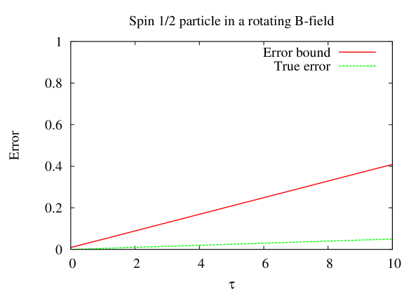
Figure 1: A plot of the error bound $\chi(\tau)$ for parameters $\theta=0.001$, $\omega=10$, and $\omega_{0}=-10$, compared to the true error for the Tong et al. [23] example. We can see that the adiabatic approximation gets worse as $\tau$ gets larger, as observed by Tong et al. [23]. However, our error bound from AT-Noise remains valid.

Figure 1 illustrates our result. Not only is the bound consistent with the true error, it has the same qualitative behavior, increasing linearly with $\tau$.

4 Application to a Superconducting Flux Qubit

Next we apply AT-Noise to the superconducting flux qubit of Orlando et al. [15], proposed for use in adiabatic quantum computation [11]. With this qubit, the adiabatic evolution may be as simple as monotonically varying an applied magnetic field.

Consider the four-junction qubit shown in Figure 2. We will follow the analysis of Orlando et al. [15]. The dynamical variables are the phases $\phi_{i}$ across the four Josephson junctions, however flux quantization in each loop gives us two constraints: $\phi_{1}-\phi_{2}+\phi_{3}=-2\pi f_{1}$ and $\phi_{4}-\phi_{3}=-2\pi f_{2}$, where $f_{1}$ and $f_{2}$ are the magnetic frustrations in each loop. So there are two degrees of freedom, which we define as $\phi_{p}=\left(\phi_{1}+\phi_{2}\right)/2$ and $\phi_{m}=\left(\phi_{1}-\phi_{2}\right)/2$, where $f_{a}=f_{2}$, and $f_{b}=f_{1}+f_{2}/2$. Then the Hamiltonian can be written as

$$\mathcal{H}=-\frac{\hbar^{2}}{2M_{p}}\frac{\partial^{2}}{\partial\phi_{p}^{2}}-\frac{\hbar^{2}}{2M_{m}}\frac{\partial^{2}}{\partial\phi_{m}^{2}}+U(\phi_{p},\phi_{m})\;,$$ (166)

where $M_{p}$ and $M_{m}$ are constants, and the potential $U(\phi_{p},\phi_{m})$ is defined as

$$U(\phi_{p},\phi_{m})=E_{J}\left[2+2\beta-2\cos(\phi_{p})\cos(\phi_{m})-2\beta\cos(\pi f_{a})\cos(2\pi f_{b}+2\phi_{m})\right]\;,$$ (167)

where $E_{J}$ and $\beta$ are constants.

Figure 2: (Adapted from Orlando et al. [15]) The circuit schematic for the superconducting flux qubit. The X’s represent Josephson junctions, and the main qubit loop is formed by junctions J1, J2, and J3. Junction J4 allows tuning of the effective properties of junction J2 through control of the frustration $f_{2}$.

At $f_{1}=f_{2}=1/3$, we have $f_{b}=1/2$ and $f_{a}=1/3$, and $U(\phi_{p},\phi_{m})$ has minima, or wells, at $\phi_{p}=0$ and $\phi_{m}=\pm\cos^{-1}(\beta/2)$, symmetric about the $\phi_{p}$ axis. By varying $f_{1}$ and $f_{2}$, we can tilt the potential so that one well is deeper than the other, and we can adjust the barrier height. We can approximate the Hamiltonian with a two-state system. A Hamiltonian evolution that begins at the degeneracy point and varies $f_{1}$ can can be written:

$$\mathcal{H}(s) =-t_{1}\sigma_{x}+s\epsilon r_{1}\sigma_{z}\;,$$ (168)

where $t_{1}$ and $r_{1}$ are parameters that can be estimated with the WKB approximation. For the qubit parameters recommended by Orlando et al. [15], $r_{1}=4.8E_{J}$ and $t_{1}=10^{-3}E_{J}$, where $E_{J}$ is a constant. A typical value for $E_{J}$ is $200\;{\rm GHz}\cdot h=1.256\;{\rm THz}\cdot\hbar$. We choose $\epsilon=-.0002$, so that the Hamiltonian changes from proportional to $\sigma_{x}$ at $s=0$ to equally-weighted $\sigma_{x}$ and $\sigma_{z}$ terms at $s=1$, because this seems a natural milestone in the evolution to the $\sigma_{z}$-dominated final Hamiltonian.

There are a couple of sources of noise in this qubit. One source of noise in a superconducting flux qubit is noise in the critical current of the Josephson junctions[26], which decreases as $1/T$ where $T$ is temperature. Such noise would result in variations in the weights of the terms in Equation (167). Another source is noise in the magnetic flux bias generated by nearby current-carrying wires on the chip. Current carrying wires could be used for nearby measurement devices or to perform a gate operation on the qubit with an RF pulse. Since we have from above a two-state Hamiltonian parametrized by flux bias, we consider this latter noise. Orlando et al. [15] estimated that a nearby wire of typical dimensions and carrying 100nA current would cause a difference in either $f_{1}$ or $f_{2}$ of $\Delta f=10^{-7}$. Let us assume that there is there is approximately $0.5\;{\rm nA}$ of noise on the wire introduced by the current source. Further suppose the power of the noise scales as inverse frequency $1/\nu$ from $\nu_{min}=2.5\;{\rm GHz}$ to $\nu_{max}=3.5\;{\rm GHz}$, so that we include the qubit frequencies throughout the evolution.

There are clever means of simulating $1/\nu$ noise with discrete models, such as by summing independent bistable fluctuators (a.k.a. Random Telegraph Noise) [6]. However, this results in non-differentiable Hamiltonians so is not appropriate for us. Instead, suppose we want to write down a formula for a noise source with $1/\nu$ power spectrum in the range $\nu_{min}$ to $\nu_{max}$. Let $n$ be an integer, with $n=100$ in the following example. Define $\Delta\nu=(\nu_{max}-\nu_{min})/n$ and $\nu_{j}=\nu_{min}+j\Delta\nu$ for $j=1...n$. Then we can define two independent noise functions, representing variation in the magnetic frustration in our qubit, as

$$\mathcal{N}_{1}(t)=C\sum_{j=1}^{n}\frac{\cos(2\pi\nu_{j}t+\xi_{1,j})\Delta\nu}{\sqrt{\nu_{j}}}\;,$$ (169)

$$\mathcal{N}_{2}(t)=C\sum_{j=1}^{n}\frac{\cos(2\pi\nu_{j}t+\xi_{2,j})\Delta\nu}{\sqrt{\nu_{j}}}$$ (170)

where $\xi_{1,j}$ and $\xi_{2,j}$ are phase factors chosen uniformly at random and $C=10^{-10}\;{\rm MHz^{-1/2}}$, chosen to agree with the $0.5\;{\rm nA}$ noise. The Hamiltonian for noise in the magnetic frustration is

$$\mathcal{H}_{noise}(t) =\mathcal{N}_{1}(t)r_{1}\sigma_{z}+N_{2}(t)(r_{2}\sigma_{z}-w\sigma_{x})\;,$$ (171)

where $w=2.4E_{J}$ for the chosen qubit parameters.

Evaluating the functions numerically over an interval much larger than the longest wavelength reveals the bounds $\left|\mathcal{N}_{i}(t)\right|\leq 4.9100\cdot 10^{-10}$, $\left|\dot{\mathcal{N}}_{i}(t)\right|\leq 9.1100\cdot 10^{-6}\;{\rm MHz}$, and $\left|\ddot{\mathcal{N}}_{i}(t)\right|\leq 0.1667\;{\rm MHz}^{2}$.

Recalling that $t=s\tau$, where $s$ is unitless, we are ready to compute derivatives and norms of the whole Hamiltonian:

$$\mathcal{H}_{\tau}(s) =\mathcal{H}(s)+\mathcal{H}_{noise}(s\tau)$$ (172)

$$=-t_{1}\sigma_{x}+sr_{1}\epsilon\sigma_{z}+\mathcal{N}_{1}(t)r_{1}\sigma_{z}+\mathcal{N}_{2}(t)\left(r_{2}\sigma_{z}-w\sigma_{x}\right)\;,$$ (173)

$$\left|\left|\dot{\mathcal{H}}_{\tau}(s)\right|\right| =\left|\left|r_{1}\epsilon\sigma_{z}+\tau\frac{d}{dt}\mathcal{N}_{1}(t)r_{1}\sigma_{z}+\tau\frac{d}{dt}\mathcal{N}_{2}(t)(r_{2}\sigma_{z}-w\sigma_{x})\right|\right|\;,$$ (174)

$$\leq 1206.4\;{\rm MHz}+\tau\cdot 84.7149\;{\rm MHz}^{2}\;,$$ (175)

$$\left|\left|\ddot{\mathcal{H}}_{\tau}(s)\right|\right| =\left|\left|\tau^{2}\frac{d^{2}}{dt^{2}}\mathcal{N}_{1}(t)r_{1}\sigma_{z}+\tau^{2}\frac{d^{2}}{dt^{2}}\mathcal{N}_{2}(t)(r_{2}\sigma_{z}-w\sigma_{x})\right|\right|\;,$$ (176)

$$\leq\tau^{2}\;1.5502\cdot 10^{6}\;{\rm MHz}^{3}\;.$$ (177)

Observe that since $s$ is unitless, $\mathcal{H}(s)$ and its $s$-derivatives all have units of energy, but since $\hbar=1$, energy units are inverse time units.

We also need to compute the minimum energy gap. In this case, it occurs at $s=0$, and the energy gap is $\bar{\gamma}_{noise}=2t_{1}=2513\;{\rm MHz}$.

Finally, we need to find $\delta_{0}$ and $\delta_{1}$. We compute the projection operators directly and obtain the bounds $\delta_{0}=1.800\cdot 10^{-6}$ and $\delta_{1}=9.117\cdot 10^{-7}$. From AT-Noise, we have

$$\left|\left|Q_{\tau}(s)U_{\tau}(s)P(0,\tau)\right|\right|\leq 1.9634\;\tau+0.0019+\frac{0.0148}{\tau}\;,$$ (178)

where if $\tau$ is supplied in microseconds, the resulting bound is unitless.

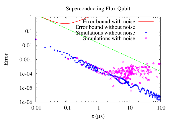
Figure 3: A plot of the error bound $\chi(\tau)$ for the superconducting flux qubit example. The crosses represent results of numerical simulations of the error. Since the noise commutes with the dominant term in the final Hamiltonian, the bound is a substantial overestimate. Nonetheless the qualitative shape between the bound curve and the simulation data agree.

This generates a hyperbolic curve with a vertical asymptote at $\tau=0$ and a linear asymptote for large $\tau$, shown in Figure 3. Recall this curve represents the norm of the error operator and its square represents the probability of error in this system.

To check our results, we would like to compute the error of the adiabatic approximation numerically. However efficient numerical simulation of this system requires some care. A straightforward solution to Schrödinger’s equation

$$i\frac{d}{dt}|\psi(t)\rangle=\mathcal{H}_{\tau}(t/\tau)|\psi(t)\rangle$$ (179)

in the $\sigma_{z}$ basis will have rapidly oscillating phases that make the solutions very unstable and time-consuming to compute. Instead, we will rewrite Schrödinger’s equation for this system in a basis whose phase rotates with time.

To begin, we choose a time-dependent eigenbasis of $\mathcal{H}_{\tau}(t/\tau)$ with the property
$\langle\phi_{n}(t)|\dot{\phi}_{n}(t)\rangle=0$. In other words, the Berry phase, also known as geometric phase, is zero.

Lemma 4.1.

There is a time dependent eigenbasis $\left\{|\phi_{n}(t)\rangle\right\}$ with the property that
$\langle\phi_{n}(t)|\dot{\phi}_{n}(t)\rangle=0$ for all $n$ [4].

Proof.

Suppose $\left\{|\phi_{n}(t)\rangle\right\}$ does not have this property. Then for each $n$, define the variable $\xi_{n}(t)$ as follows:

$$\xi_{n}(t)=i\int_{0}^{t}\langle\phi_{n}(w)|\dot{\phi}_{n}(w)\rangle dw$$ (180)

and let

$$|\alpha_{n}(t)\rangle=e^{i\xi_{n}(t)}|\phi_{n}(t)\rangle\;.$$ (181)

Then $\left\{|\alpha_{n}(t)\rangle\right\}$ has the desired property. To see this, we simply compute it:

$$\langle\alpha_{n}(t)|\dot{\alpha_{n}}(t)\rangle =\langle\phi_{n}(t)|e^{-i\xi_{n}(t)}\left[i\dot{\xi}_{n}(t)e^{i\xi_{n}(t)}|\phi_{n}(t)\rangle+e^{i\xi_{n}(t)}|\dot{\phi}_{n}(t)\rangle\right]$$ (182)

$$=i\dot{\xi}_{n}(t)+\langle\phi_{n}(t)|\dot{\phi}_{n}(t)\rangle$$ (183)

$$=i\cdot i\langle\phi_{n}(t)|\dot{\phi}_{n}(t)\rangle+\langle\phi_{n}(t)|\dot{\phi}_{n}(t)\rangle$$ (184)

$$=0\;.$$ (185)

∎

Let us write the solution $|\psi(t)\rangle$ in terms of the basis states $|\phi_{n}(t)\rangle$ with energies $E_{n}(t)$ as follows:

$$|\psi(t)\rangle=\sum_{n}c_{n}(t)e^{-i\int_{0}^{t}E_{n}(w)dw}|\phi_{n}(t)\rangle\;.$$ (186)

Then in the case of two states, assuming the eigenstates are labeled in increasing order with respect to their eigenvalues, the norm of the adiabatic error operator is simply $\left|c_{1}(t)\right|$.

Let us substitute the representation in Equation (186) into Schrödinger’s equation (Equation (179)), and left multiply by $\langle\phi_{m}(t)|$. After simplification, this yields

$$\dot{c}_{m}(t)=-\sum_{n}c_{n}(t)e^{-i\int_{0}^{t}\left(E_{n}(w)-E_{m}(w)\right)dw}\langle\phi_{m}(t)|\dot{\phi}_{n}(t)\rangle\;.$$ (187)

Evidently the $n=m$ term in the sum is zero in the chosen basis.

Since we have

$$\mathcal{H}_{\tau}(t/\tau) =\left(-t_{1}-\mathcal{N}_{2}(t)s_{2}\right)\sigma_{x}+\left(\frac{t\;r_{1}\;\epsilon}{\tau}+\mathcal{N}_{1}(t)r_{1}+\mathcal{N}_{2}(t)r_{2}\right)\sigma_{z}\;,$$ (188)

if we define

$$a(t) =-t_{1}-\mathcal{N}_{2}(t)s_{2}\;,$$ (189)

$$b(t) =\frac{t\;r_{1}\;\epsilon}{\tau}+\mathcal{N}_{1}(t)r_{1}+\mathcal{N}_{2}(t)r_{2}\;,$$ (190)

$$\theta(t) =\cot^{-1}\left(\frac{b(t)}{a(t)}\right)\;,$$ (191)

then we can diagonalize the Hamiltonian easily in terms of $a(t)$ and $b(t)$. We choose the cotangent for numerical stability because $b(0)\approx 0$.

$$E_{0}(t) =-\sqrt{a^{2}(t)+b^{2}(t)} E_{1}(t) =\sqrt{a^{2}(t)+b^{2}(t)}$$ (192)

$$|\phi_{0}(t)\rangle =\left(\begin{array}[]{c}-\sin\left(\frac{\theta(t)}{2}\right)\\ \cos\left(\frac{\theta(t)}{2}\right)\end{array}\right) |\phi_{1}(t)\rangle =\left(\begin{array}[]{c}\cos\left(\frac{\theta(t)}{2}\right)\\ \sin\left(\frac{\theta(t)}{2}\right)\end{array}\right)\;.$$ (197)

Now, we would like to compute $\langle\phi_{0}(t)|\dot{\phi}_{1}(t)\rangle$ and $\langle\phi_{1}(t)|\dot{\phi}_{0}(t)\rangle$.

$$\langle\phi_{0}(t)|\dot{\phi}_{1}(t)\rangle =\left(\begin{array}[]{c}-\sin\left(\frac{\theta(t)}{2}\right)\\ \cos\left(\frac{\theta(t)}{2}\right)\end{array}\right)\cdot\left(\begin{array}[]{c}-\frac{1}{2}\sin\left(\frac{\theta(t)}{2}\right)\dot{\theta}(t)\\ \frac{1}{2}\cos\left(\frac{\theta(t)}{2}\right)\dot{\theta}(t)\end{array}\right)$$ (202)

$$=\frac{\dot{\theta}(t)}{2}$$ (203)

$$\langle\phi_{1}(t)|\dot{\phi}_{0}(t)\rangle =\left(\begin{array}[]{c}\cos\left(\frac{\theta(t)}{2}\right)\\ \sin\left(\frac{\theta(t)}{2}\right)\end{array}\right)\cdot\left(\begin{array}[]{c}-\frac{1}{2}\cos\left(\frac{\theta(t)}{2}\right)\dot{\theta}(t)\\ -\frac{1}{2}\sin\left(\frac{\theta(t)}{2}\right)\dot{\theta}(t)\end{array}\right)$$ (208)

$$=-\frac{\dot{\theta}(t)}{2}$$ (209)

It remains to compute $\dot{\theta}(t)$, which can be done with implicit differentiation.

$$\cot(\theta(t)) =\frac{b(t)}{a(t)}$$ (210)

$$-\csc^{2}(\theta(t))\dot{\theta}(t) =\frac{\dot{b}(t)a(t)-b(t)\dot{a}(t)}{a^{2}(t)}$$ (211)

$$\dot{\theta}(t) =\sin^{2}(\theta(t))\frac{\dot{a}(t)b(t)-a(t)\dot{b}(t)}{a^{2}(t)}$$ (212)

$$=\frac{a^{2}(t)}{a^{2}(t)+b^{2}(t)}\frac{\dot{a}(t)b(t)-a(t)\dot{b}(t)}{a^{2}(t)}$$ (213)

$$=\frac{\dot{a}(t)b(t)-a(t)\dot{b}(t)}{a^{2}(t)+b^{2}(t)}$$ (214)

Finally, the equations of motion are

$$\dot{c}_{0}(t) =-c_{1}(t)e^{-2i\int_{0}^{t}\sqrt{a^{2}(w)+b^{2}(w)}dw}\frac{\dot{\theta}(t)}{2}$$ (215)

$$\dot{c}_{1}(t) =c_{0}(t)e^{2i\int_{0}^{t}\sqrt{a^{2}(w)+b^{2}(w)}dw}\frac{\dot{\theta}(t)}{2}$$ (216)

We provide these equations to a differential equation solver, ode23, in Matlab. Care must be taken with the integral in the exponent. We need not recompute the integral entirely at each time; rather we cache the intermediate values of this integral. Thus at each evaluation we only integrate on the interval from the last cached time to the current time.

This method was used to produce the numeric results in Figure 3. The parameters of the system are those previously described in the example. There are 571 noiseless data points and 125 noisy data points. A new set of random phases was generated for each noisy point, and each point took up to 5.5 CPU hours to compute. The workstation used had dual Xeon 3.06 GHZ processors with hyperthreading enabled (thus four effective CPUs) and 6GB of RAM, running Red Hat Enterprise 3.

The simulation data in Figure 3 is several orders of magnitude less than the bound. The fact that the bound is an overestimate is not surprising since the noise term commutes with the dominant term in the final Hamiltonian of the evolution. However the qualitative shape between the bound curve and the simulation data is the same, and the bound does provide a simulation-free guarantee of error for an interval of $\tau$.

5 Conclusion

We provide rigorous bounds for the adiabatic approximation under for four sources of experimental error: perturbations in the initial condition, systematic time-dependent perturbations in the Hamiltonian, coupling to low-energy quantum systems, and decoherent time-dependent perturbations in the Hamiltonian.

We applied the new results to the spin-1/2 particle in a rotating magnetic field, which is a standard example for discussing controversy in the adiabatic theorem [4, 23, 27]. We showed that our theorem makes correct predictions about the error of the adiabatic approximation as a function of time.

We also applied the new results to the superconducting flux qubit proposed by Orlando et al. [15], with time-dependent perturbations in the applied magnetic field. This qubit has properties that make it a candidate for quantum adiabatic computation [11]. Because our version of the adiabatic theorem does not have unspecified constants, we are able to make numerical predictions about this qubit. We showed that for a particular amount of noise on superconducting wires near a qubit with ideal physical parameters, we could guarantee a small error in the adiabatic approximation provided that the evolution time was set within a particular interval.

6 Acknowledgments

The authors would like to thank Stephen Bullock, P. Aaron Lott, Ben Reichardt, Jocelyn Rodgers, and Eite Tiesinga for helpful comments and feedback.

NIST disclaimer. Certain commercial products may be identified in this paper to specify experimental procedures. Such identification is not intended to imply recommendation or endorsement by the National Institute of Standards and Technology.

Appendix Appendix A: Proof of the Adiabatic Theorem

Our proof of the adiabatic theorem follows closely those by Avron et al. [2] (later corrections exist [3] [12]), Reichardt [16], and Jansen et al. [10]. The purpose of revisiting the proof is to have explicit definitions of constants.

After reviewing some properties of projection operators, we will introduce the version of Schrödinger’s equation that will be used and the assumptions that it requires. Then we will introduce some essential lemmas, and finally the proof.

A.1 Properties of projection operators

Before embarking on the proof, it will be helpful to review some properties of projection operators. First, we will enumerate some elementary properties. Then, we will introduce the resolvent formalism for rewriting projection operators as a contour integral.

Define the commutator $[A,B]$ as $[A,B]=AB-BA$, and $\dot{A}=dA/ds$. Let $\mathcal{H}(s)$ be some Hamiltonian with countable eigenstates $\{|\psi_{j}(s)\rangle\}$ and eigenvalues $\{\lambda_{j}(s):j\geq 0\}$. Let $P(s)$ be the orthogonal projection operator onto the subspace

$$\Psi(s)={\rm Span}\left\{|\psi_{m}(s)\rangle,...,|\psi_{n}(s)\rangle\right\}\;,$$ (A-1)

for some $0\leq m\leq n$. Thus

$$P(s)=\sum_{i=0}^{k}|\psi_{i}(s)\rangle\langle\psi_{i}(s)|\;.$$ (A-2)

Let $Q(s)=I-P(s)$ be the orthogonal complement of $P(s)$. Then the following properties hold:

1. $P(s)=P^{2}(s)$.

2. $\dot{P}(s)=\dot{P}(s)P(s)+P(s)\dot{P}(s)$, obtained by differentiating both sides of Property (1).

3. $P(s)\dot{P}(s)P(s)=0$, obtained by multiplying Property (2) from the left by $P$.

4. $Q(s)P(s)=0$, using the definition of $Q$ and Property (1).

5. $P^{\dagger}(s)=P(s)$ and $Q^{\dagger}(s)=Q(s)$, where ^† indicates the conjugate transpose. This is evident from Equation (A-2).

6. $\left|\left|P(s)\right|\right|=\left|\left|Q(s)\right|\right|=1$. Recall that the norm of an operator $P(s)$ is defined to be the maximum of $\left|\left|P(s)|x\rangle\right|\right|$ for choices of normalized states $|x\rangle$. For a projection operator, the maximal choice is a vector in the plane of projection, and in that case $P(s)|x\rangle=|x\rangle$. So $\left|\left|P(s)\right|\right|=1$. For $Q(s)$, choose $|x\rangle$ orthogonal to the plane of projection.

7. $[\mathcal{H}(s),P(s)]=0$. To prove this, take some state $|\phi\rangle$ and rewrite it as $|\phi\rangle=\sum_{j\geq 0}c_{j}|\psi_{j}(s)\rangle$. Then

   $$\mathcal{H}(s)P(s)|\phi\rangle =\sum_{j\geq 0}c_{j}\mathcal{H}(s)P(s)|\psi_{j}(s)\rangle$$ (A-3)

   $$=\sum_{j=m}^{n}c_{j}\mathcal{H}(s)|\psi_{j}(s)\rangle$$ (A-4)

   $$=\sum_{j=m}^{n}c_{j}\lambda_{j}(s)|\psi_{j}(s)\rangle$$ (A-5)

   and

   $$P(s)\mathcal{H}(s)|\phi\rangle =\sum_{j=m}^{n}P(s)\mathcal{H}(s)c_{j}|\psi_{j}(s)\rangle+\sum_{j\not\in[m,n]}P(s)\mathcal{H}(s)c_{j}|\psi_{j}(s)\rangle$$ (A-6)

   $$=\sum_{j=m}^{n}c_{j}P(s)\lambda_{j}(s)|\psi_{j}(s)\rangle+\sum_{j\not\in[m,n]}c_{j}P(s)\lambda_{j}(s)|\psi_{j}(s)\rangle$$ (A-7)

   $$=\sum_{j=m}^{n}c_{j}\lambda_{j}(s)|\psi_{j}(s)\rangle\;.$$ (A-8)

We will make use of the resolvent formalism to bound the projection operators. Define the resolvent of a Hamiltonian $\mathcal{H}(s)$ to be

$$R(z;\mathcal{H}(s))=(\mathcal{H}(s)-zI)^{-1}\;.$$ (A-9)

Suppose we can draw a contour $\Gamma(s)$ in the complex plane whose enclosed region includes the eigenvalues corresponding to $\Psi(s)$ and excludes the rest of the spectrum of $\mathcal{H}(s)$. Then we can rewrite the projection operator $P(s)$ in terms of a line integral of the resolvent $R(s,z)=(\mathcal{H}(s)-zI)^{-1}$ around this contour:

$$P(s)=-\frac{1}{2\pi i}\oint_{\Gamma(s)}R(s,z)dz\;.$$ (A-10)

A.2 Schrödinger’s equation

We rewrite Schrödinger’s equation in terms of unitary evolution operators and the scaled time $s$, rather than using state vectors and real time $t$. Doing so will introduce the assumption that $\mathcal{H}(s)$ has a continuous, bounded second derivative.

The usual expression of the time-dependent Schrödinger’s equation is

$$i\hbar\frac{d|\psi(t)\rangle}{dt}=\mathcal{H}(t)|\psi(t)\rangle\;.$$ (A-11)

Setting $t=s\tau$, $|\phi(s)\rangle=|\psi(s\tau)\rangle=|\psi(t)\rangle$, and $\mathcal{H}_{\tau}(s)=\mathcal{H}(s\tau)=\mathcal{H}(t)$, we can substitute and apply the chain rule for derivatives to get

$$\hbar|\dot{\phi}(s)\rangle =-i\tau\mathcal{H}_{\tau}(s)|\phi(s)\rangle\;,$$ (A-12)

where the dot indicates the $s$-derivative. It will be convenient in this proof to choose our units so that $\hbar=1$. Also we will assume that all subsequent state vectors, Hamiltonians, and time evolution operators are functions of the normalized time parameter $s$, so we can drop the subscript $\tau$ from $\mathcal{H}_{\tau}$. Thus we will write

$$|\dot{\phi}(s)\rangle =-i\tau\mathcal{H}(s)|\phi(s)\rangle\;.$$ (A-13)

Now define $U(s)$ so that for any $|\phi(0)\rangle$, we have $U(s)|\phi(0)\rangle=|\phi(s)\rangle$ where $|\phi(s)\rangle$ is the solution to this equation. Then we proceed as in [18]. Assume that $\mathcal{H}(s)$ has a continuous bounded derivative; then $|\phi(s)\rangle$ has a continuous bounded second derivative. Thus the remainder for the first-order Taylor expansion is well-defined. For some point $s^{*}\in[s,s+\Delta s]$, we get

$$U(s+\Delta s)|\phi(0)\rangle =|\phi(s+\Delta s)\rangle$$ (A-14)

$$=|\phi(s)\rangle+|\dot{\phi}(s)\rangle\Delta s+|\ddot{\phi}(s^{*})\rangle\frac{\Delta s^{2}}{2}$$ (A-15)

$$=|\phi(s)\rangle-i\tau\mathcal{H}(s)|\phi(s)\rangle\Delta s+\mathcal{O}(\Delta s^{2})$$ (A-16)

$$=U(s)|\phi(0)\rangle-i\tau\mathcal{H}(s)U(s)|\phi(0)\rangle\Delta s+\mathcal{O}(\Delta s^{2})\;.$$ (A-17)

Since this is true for any $|\phi(0)\rangle$ we can write

$$\lim_{\Delta s\rightarrow 0}\frac{U(s+\Delta s)-U(s)}{\Delta s} =-i\tau\mathcal{H}(s)U(s)$$ (A-18)

or, equivalently,

$$\dot{U}(s) =-i\tau\mathcal{H}(s)U(s)\;.$$ (A-19)

Equation (A-19) is the form of Schrödinger’s equation that we will rely on for the rest of the proof of the adiabatic theorem.

A.3 Essential Lemmas

Recall that the adiabatic approximation states that a system of Hamiltonian $\mathcal{H}(s)$, initially in some state in $\Psi(0)$, evolves to approximately some state in $\Psi(s)$ at time $t=s\tau$. To compute bounds on the error of this approximation, we will identify a Hamiltonian $\mathcal{H}_{A}$ that has exactly this property. Define

$$\mathcal{H}_{A}(s)=\mathcal{H}(s)+\frac{i}{\tau}\left[\dot{P}(s),P(s)\right]$$ (A-20)

where $P(s)$ is the projection operator onto $\Psi(s)$. Evidently $\mathcal{H}_{A}$ is a $1/\tau$ perturbation of $\mathcal{H}$, where $\tau$ is the scale factor between normalized time and unnormalized time. Define $U_{A}(s)$ to be the unitary evolution operator that is the solution to Schrödinger’s equation for $\mathcal{H}_{A}$, namely

$$\dot{U}_{A}(s)=-i\tau\mathcal{H}_{A}(s)U_{A}(s)\;.$$ (A-21)

The important property of $\mathcal{H}_{A}(s)$ can be restated as follows. If a system is initialized in $\Psi(0)$ at time $s=0$, the state at time $s$ under evolution by the Hamiltonian $\mathcal{H}_{A}(s)$ is entirely contained in $\Psi(s)$. We can write this property, known as the intertwining property, using $P(s)$ and $U_{A}(s)$ as defined in the previous paragraph.

Theorem A.1 (The Intertwining Property).

For all $0\leq s\leq 1$, let $\mathcal{H}(s)$ be Hermitian, twice differentiable, non-degenerate, and have a countable number of eigenstates. Let $U_{A}(s)$ and $P(s)$ be defined as previously. Then

$$U_{A}(s)P(0)=P(s)U_{A}(s)\;.$$ (A-22)

Proof.

Noticing that $U_{A}(s)$ is unitary, we can rewrite the claim as $P(0)=U_{A}^{\dagger}(s)P(s)U_{A}(s)$. Since $U_{A}(0)=I$ this is certainly true for $s=0$. So it is sufficient to show that

$$\frac{d}{ds}\left[U_{A}^{\dagger}(s)P(s)U_{A}(s)\right] =0\;.$$ (A-23)

Applying the product rule for derivatives we get

$$\frac{d}{ds}\left[U_{A}^{\dagger}(s)P(s)U_{A}(s)\right] =\frac{d}{ds}\left[U_{A}^{\dagger}(s)P(s)\right]U_{A}(s)+U_{A}^{\dagger}(s)P(s)\dot{U}_{A}(s)$$ (A-24)

$$=\left(U_{A}^{\dagger}(s)\dot{P}(s)+\dot{U_{A}^{\dagger}}(s)P(s)\right)U_{A}(s)+U_{A}^{\dagger}(s)P(s)\dot{U}_{A}(s)\;.$$ (A-25)

Now observe that $\dot{U_{A}^{\dagger}}=(\dot{U}_{A})^{\dagger}$ since the derivative of a matrix operator is the derivative of its matrix entries. Further, recall that $\dot{U}_{A}(s)=-i\tau\mathcal{H}_{A}(s)U_{A}(s)$. So

$$\dot{U_{A}^{\dagger}}(s) =(\dot{U}_{A}(s))^{\dagger}$$ (A-26)

$$=\left(-i\tau\mathcal{H}_{A}(s)U_{A}(s)\right)^{\dagger}$$ (A-27)

$$=+i\tau U_{A}^{\dagger}(s)\mathcal{H}_{A}^{\dagger}(s)$$ (A-28)

$$=i\tau U_{A}^{\dagger}(s)\mathcal{H}_{A}(s)\;,$$ (A-29)

since $\mathcal{H}_{A}$ is Hermitian. Substituting, we get

$$\frac{d}{ds}\left[U_{A}^{\dagger}(s)P(s)U_{A}(s)\right]= \left(U_{A}^{\dagger}(s)\dot{P}(s)+i\tau U_{A}^{\dagger}(s)\mathcal{H}_{A}(s)P(s)\right)U_{A}(s)$$

$$+U_{A}^{\dagger}(s)P(s)(-i)\tau\mathcal{H}_{A}(s)U_{A}(s)$$ (A-30)

$$= U_{A}^{\dagger}(s)\left(\dot{P}(s)+i\tau\mathcal{H}_{A}(s)P(s)-i\tau P(s)\mathcal{H}_{A}(s)\right)U_{A}(s)$$ (A-31)

$$= U_{A}^{\dagger}(s)\left(\dot{P}(s)+i\tau[\mathcal{H}_{A}(s),P(s)]\right)U_{A}(s)\;.$$ (A-32)

Now we will work on the inner term. We use the properties that $[H(s),P(s)]=0$, $P(s)\dot{P}(s)P(s)=0$, $P^{2}(s)=P(s)$, and $\dot{P}(s)=\dot{P}(s)P(s)+P(s)\dot{P}(s)$.

$$[\mathcal{H}_{A}(s),P(s)]= \mathcal{H}_{A}(s)P(s)-P(s)\mathcal{H}_{A}(s)$$ (A-33)

$$= \left(\mathcal{H}(s)+\frac{i}{\tau}\left(\dot{P}(s)P(s)-P(s)\dot{P}(s)\right)\right)P(s)$$

$$-P(s)\left(\mathcal{H}(s)+\frac{i}{\tau}\left(\dot{P}(s)P(s)-P(s)\dot{P}(s)\right)\right)$$ (A-34)

$$= [\mathcal{H}(s),P(s)]+\frac{i}{\tau}\dot{P}(s)P^{2}(s)-\frac{i}{\tau}P(s)\dot{P}(s)P(s)$$

$$-\frac{i}{\tau}P(s)\dot{P}(s)P(s)+\frac{i}{\tau}P^{2}(s)\dot{P}(s)$$ (A-35)

$$= \frac{i}{\tau}\dot{P}(s)P^{2}(s)+\frac{i}{\tau}P^{2}(s)\dot{P}(s)$$ (A-36)

$$= \frac{i}{\tau}\dot{P}(s)P(s)+\frac{i}{\tau}P(s)\dot{P}(s)$$ (A-37)

$$= \frac{i}{\tau}\dot{P}(s)\;.$$ (A-38)

We can substitute this into the original expression to get

$$\frac{d}{ds}\left[U_{A}^{\dagger}(s)P(s)U_{A}(s)\right] =U_{A}^{\dagger}(s)\left(\dot{P}(s)+i\tau[\mathcal{H}_{A}(s),P(s)]\right)U_{A}(s)$$ (A-39)

$$=U_{A}^{\dagger}(s)\left(\dot{P}(s)-\dot{P}(s)\right)U_{A}(s)$$ (A-40)

$$=0\;.$$ (A-41)

∎

Notice that this implies an intertwining property for the orthogonal complement:

$$U_{A}(s)Q(0)=Q(s)U_{A}(s)\;.$$ (A-42)

In the proof of the adiabatic theorem we will make use of the twiddle operation. For a fixed $s$, let $P$ be a projection operator onto $\Psi(s)$, and assume the eigenvalues corresponding to $\Psi(s)$ are separated by a gap from the rest of the eigenvalues. Define

$$\tilde{X}(s)=\frac{1}{2\pi i}\oint_{\Gamma(s)}R(s,z)X(s)R(s,z)dz$$ (A-43)

where $\Gamma(s)$ is a contour in the complex plane around the eigenvalues associated with the eigenstates onto which $P(s)$ projects, whose enclosed region excludes any other eigenvalues of $\mathcal{H}(s)$. We will need the following property of the twiddle operation.

Lemma A.2 (The Twiddle Lemma).

Assume $\hbar=1$. For a fixed $s$, let $P$ be a projection operator onto $\Psi(s)$, and assume the eigenvalues corresponding to $\Psi(s)$ are separated by a gap from the rest of the eigenvalues. Define $Q=I-P$, and let $X$ be a bounded linear operator. Then

$$QXP=-Q\left(\left[\mathcal{H}_{A},\tilde{X}\right]-\frac{i}{\tau}\left[\dot{P},\tilde{X}\right]\right)P$$ (A-44)

Proof.

We begin by observing that since $P^{2}=P$ and $QP=0$,

$$-Q[X,P]P =-Q(XP-PX)P$$ (A-45)

$$=-QXP\;.$$ (A-46)

Further, since the identity operator commutes with everything, $[zI,R(z)XR(z)]=0$. Then

$$[\mathcal{H},\tilde{X}] =\mathcal{H}\left(\frac{1}{2\pi i}\oint_{\Gamma}R(z)XR(z)dz\right)-\left(\frac{1}{2\pi i}\oint R(z)XR(z)dz\right)\mathcal{H}$$ (A-47)

$$=\frac{1}{2\pi i}\oint_{\Gamma}\left(\mathcal{H}R(z)XR(z)-R(z)XR(z)\mathcal{H}\right)dz$$ (A-48)

$$=\frac{1}{2\pi i}\oint_{\Gamma}[\mathcal{H},R(z)XR(z)]dz$$ (A-49)

$$=\frac{1}{2\pi i}\oint_{\Gamma}[\mathcal{H}-zI,R(z)XR(z)]dz$$ (A-50)

Now we use the fact that $(\mathcal{H}-zI)R=I$, that $X$ does not depend on $z$, and Equation (A-10) to write

$$[\mathcal{H},\tilde{X}] =\frac{1}{2\pi i}\oint_{\Gamma}\left(XR(z)-R(z)X\right)dz$$ (A-51)

$$=\frac{1}{2\pi i}[X,\oint_{\Gamma}R(z)dz]$$ (A-52)

$$=-[X,P]\;.$$ (A-53)

Also, using the definition of $\mathcal{H}_{A}$ in (A-20), we have

$$QXP =Q[X,P]P$$ (A-54)

$$=-Q[\mathcal{H},\tilde{X}]P$$ (A-55)

$$=-Q\left(\left[\mathcal{H}_{A},\tilde{X}\right]-\frac{i}{\tau}\left[\left[\dot{P},P\right],\tilde{X}\right]\right)P\;.$$ (A-56)

All we need to finish the proof is to show

$$Q\left[\left[\dot{P},P\right],\tilde{X}\right]P=Q\left[\dot{P},\tilde{X}\right]P\;.$$ (A-57)

Using $P\dot{P}P=0$, $P^{2}=P$, and $\dot{P}=\dot{P}P+P\dot{P}$, we have

$$Q[[\dot{P},P]\tilde{X}]P =Q[\dot{P}P-P\dot{P},\tilde{X}]P$$ (A-58)

$$=Q\left(\dot{P}P-P\dot{P}\right)\tilde{X}P-Q\tilde{X}\left(\dot{P}P-P\dot{P}\right)P$$ (A-59)

$$=(I-P)\left(\dot{P}P-P\dot{P}\right)\tilde{X}P-(I-P)\tilde{X}\left(\dot{P}P-P\dot{P}\right)P$$ (A-60)

$$=\dot{P}P\tilde{X}P-P\dot{P}\tilde{X}P+P\dot{P}\tilde{X}P-\tilde{X}\dot{P}P+P\tilde{X}\dot{P}P$$ (A-61)

$$=\dot{P}\tilde{X}P-P\dot{P}\tilde{X}P-\tilde{X}\dot{P}P+P\tilde{X}\dot{P}P$$ (A-62)

$$=(I-P)\dot{P}\tilde{X}P-(I-P)\tilde{X}\dot{P}P$$ (A-63)

$$=Q\dot{P}\tilde{X}P-Q\tilde{X}\dot{P}P$$ (A-64)

$$=Q[\dot{P},\tilde{X}]P\;.$$ (A-65)

∎

A.4 Completion of the Proof

Now we are ready to prove the adiabatic theorem. The operator $Q(s)U(s)P(0)$ takes the $\Psi(0)$ component of a state vector, and evolves it for (normalized) time $s$ under $\mathcal{H}(s)$, then computes the error from the adiabatic approximation. The theorem guarantees an upper bound on the norm of this operator.

Theorem A.3 (The Adiabatic Theorem).

Assume for $0\leq s\leq 1$ that $\mathcal{H}(s)$ is twice differentiable, and let

$$\left|\left|\dot{\mathcal{H}}(s)\right|\right| \leq b_{1}(s)\;, \left|\left|\ddot{\mathcal{H}}(s)\right|\right| \leq b_{2}(s)\;,$$ (A-66)

Further assume that $\mathcal{H}(s)$ has a countable number of eigenstates, with eigenvalues
$\lambda_{0}(s)\leq\lambda_{1}(s)...$, and that $P(s)$ projects onto the eigenspace associated with the eigenvalues $\{\lambda_{m}(s),\lambda_{m+1}(s),...\lambda_{n}(s)\}$. Define

$$w(s) =\lambda_{n}(s)-\lambda_{m}(s)\;, \gamma(s) =\left\{\begin{array}[]{ll}\min\{\lambda_{n+1}(s)-\lambda_{n}(s),\;\lambda_{m}(s)-\lambda_{m-1}(s)\}&m>0\\ \lambda_{n+1}(s)-\lambda_{n}(s)&m=0\end{array}\right.\;,$$ (A-69)

$$D(s) =1+\frac{2w(s)}{\pi\gamma(s)}\;, Q(s) =I-P(s)\;.$$ (A-70)

Finally, assume $\gamma(s)>0$ all $s$. Then we have

$$\left|\left|Q(s)U(s)P(0)\right|\right|\leq \frac{8D^{2}(0)b_{1}(0)}{\tau\gamma^{2}(0)}+\frac{8D^{2}(s)b_{1}(s)}{\tau\gamma^{2}(s)}$$

$$+\int_{0}^{s}\frac{8D^{2}(r)}{\tau\gamma^{2}(r)}\left(\frac{8(1+D(r))b_{1}^{2}(r)}{\gamma(r)}+b_{2}(r)\right)dr\;.$$ (A-71)

Proof.

By multiplying by the identity and applying Theorem A.1 (the intertwining property), we can write:

$$Q(s)U(s)P(0) =Q(s)U_{A}(s)U_{A}^{\dagger}(s)U(s)P(0)$$ (A-72)

$$=U_{A}(s)Q(0)U_{A}^{\dagger}(s)U(s)P(0)\;.$$ (A-73)

Since $\left|\left|U_{A}(s)\right|\right|=1$, if $\left|\left|Q(0)U_{A}^{\dagger}(s)U(s)P(0)\right|\right|$ is small the magnitude of the error in the adiabatic approximation is small. In fact, if we define

$$W(s)=U_{A}^{\dagger}(s)U(s)$$ (A-74)

then $W(s)$ satisfies a useful integral equation, and we prove the adiabatic theorem by bounding $\left|\left|Q(0)W(s)P(0)\right|\right|$ instead of working directly on $Q(s)U(s)P(0)$. To find the integral equation, we need to compute $\dot{W}(s)$. Using the product rule for derivatives, Schrödinger’s equation, and the definition of $\mathcal{H}_{A}(s)$ in (A-20), we have

$$\dot{W}(s) =U_{A}^{\dagger}(s)\dot{U}(s)+\dot{U}_{A}^{\dagger}(s)U(s)$$ (A-75)

$$=-i\tau U_{A}^{\dagger}(s)\mathcal{H}(s)U(s)+i\tau U_{A}^{\dagger}(s)\mathcal{H}_{A}(s)U(s)$$ (A-76)

$$=-U_{A}^{\dagger}(s)\left[\dot{P}(s),P(s)\right]U(s)$$ (A-77)

$$=-U_{A}^{\dagger}(s)\left[\dot{P}(s),P(s)\right]U_{A}(s)W(s)\;.$$ (A-78)

Clearly $W(0)=I$ and so

$$W(s)=I-\int_{0}^{s}U_{A}^{\dagger}(r)[\dot{P}(r),P(r)]U_{A}(r)W(r)dr$$ (A-79)

It will be useful sometimes to refer to the kernel of this integral equation, so we define

$$K(r)=U_{A}^{\dagger}(r)\left[\dot{P}(r),P(r)\right]U_{A}(r)\;.$$ (A-80)

Now we can use Equation (A-79) to rewrite $\left|\left|Q(0)W(s)P(0)\right|\right|$. Using the fact that $Q(0)P(0)=0$, we can write

$$Q(0)W(s)P(0)=-\int_{0}^{s}Q(0)K(r)W(r)P(0)dr\;.$$ (A-81)

Our plan is to rewrite the integrand to obtain an expression where all but one term has a $1/\tau$ factor. Integration by parts on the remaining term will ensure all terms have a $1/\tau$ factor. Then we can factor out the $1/\tau$ and bound the operators in each term to yield the Adiabatic Theorem.

To obtain this expression, we need to introduce a $P(0)$ in the middle of Equation (A-81) so that we can apply Lemma A.2. To do so, we will use the fact that $Q(0)=Q(0)^{2}$ to introduce another $Q(0)$, and then use the fact that $Q(0)K(r)=K(r)P(0)$.

To show that $Q(0)K(r)=K(r)P(0)$, we use intertwining properties, the fact that $Q(r)P(r)=0$, and the properties $P^{2}(r)=P(r)$ and $P(r)\dot{P}(r)P(r)=0$:

$$Q(0)K(r) =Q(0)U_{A}^{\dagger}(r)[\dot{P}(r),P(r)]U_{A}(r)$$ (A-82)

$$=U_{A}^{\dagger}(r)Q(r)[\dot{P}(r),P(r)]U_{A}(r)$$ (A-83)

$$=U_{A}^{\dagger}(r)\left(Q(r)\dot{P}(r)P(r)-Q(r)P(r)\dot{P}(r)\right)U_{A}(r)$$ (A-84)

$$=U_{A}^{\dagger}(r)Q(r)\dot{P}(r)P(r)U_{A}(r)$$ (A-85)

$$=U_{A}^{\dagger}(r)\left(\dot{P}(r)P^{2}(r)-P(r)\dot{P}(r)P(r)\right)U_{A}(r)$$ (A-86)

$$=U_{A}^{\dagger}(r)\left[\dot{P}(r),P(r)\right]P(r)U_{A}(r)$$ (A-87)

$$=U_{A}^{\dagger}(r)\left[\dot{P}(r),P(r)\right]U_{A}(r)P(0)$$ (A-88)

$$=K(r)P(0)\;.$$ (A-89)

Then we can rewrite

$$Q(0)W(s)P(0) =-\int_{0}^{s}Q(0)K(r)W(r)P(0)dr$$ (A-90)

$$=-\int_{0}^{s}Q(0)^{2}K(r)W(r)P(0)dr$$ (A-91)

$$=-\int_{0}^{s}Q(0)K(r)P(0)W(r)P(0)dr\;.$$ (A-92)

Now we use the definition of $K(r)$, the properties $P^{2}(r)=P(r)$ and $Q^{2}(r)=Q(r)$, and the intertwining property again:

$$Q(0)W(s)P(0) =-\int_{0}^{s}Q(0)^{2}U_{A}^{\dagger}(r)\left[\dot{P}(r),P(r)\right]U_{A}(r)P(0)^{2}W(r)P(0)dr$$ (A-93)

$$=-\int_{0}^{s}Q(0)U_{A}^{\dagger}(r)Q(r)\left[\dot{P}(r),P(r)\right]P(r)U_{A}(r)P(0)W(r)P(0)dr\;.$$ (A-94)

We would like to apply Lemma A.2 with

$$X(r)= \left[\dot{P}(r),P(r)\right]\;.$$ (A-95)

In order to apply the lemma, we need to show $X(r)$ is a bounded linear operator. Clearly $X(r)$ is linear, and since $P(r)$ has unit norm then it is sufficient to show that $\left|\left|\dot{P}(r)\right|\right|$ has a bound.

Figure 4: Visualization of the resolvent contour $\Gamma(s)$. The eigenvalues of $\mathcal{H}(s)$ (represented with black dots) all lie along the real axis since $\mathcal{H}(s)$ is Hermitian. Notice $\Gamma(s)$ lies at least $\gamma(s)/2$ from any eigenvalues. The length of $\Gamma(s)$ is $\pi\gamma(s)+2w(s)=D(s)\pi\gamma(s)$. Observe that $D(s)$ is the ratio of the length of $\Gamma(s)$ to the circumference of a circle of radius $\gamma(s)/2$.

To bound the norm of $\dot{P}(r)$ we will use the resolvent formalism. We first need to bound the norm of the resolvent $R(r,z)$. Notice that if the eigenstates of $\mathcal{H}(r)$ are $\{|\psi_{j}(r)\rangle:j\geq 0\}$, then

$$R(r,z)=\sum_{j\geq 0}\frac{1}{\lambda_{j}(r)-z}|\psi_{j}(r)\rangle\langle\psi_{j}(r)|\;,$$ (A-96)

so the norm of $R(r,z)$ equals the inverse of the minimum distance of $z$ to an eigenvalue of $\mathcal{H}(r)$. So we need to choose the contour $\Gamma(r)$ around the eigenvalues of $\Psi(r)$ to maximize the minimum distance of $\Gamma(r)$ to any eigenvalue. Also, to obtain the best bound on the path integral, we will want to minimize the length of $\Gamma(r)$, given that maximum minimum distance. We choose $\Gamma(r)$ consisting of two semicircles connected by lines, forming a pill-shape. The semicircles are centered at $\lambda_{m}(r)$ and $\lambda_{n}(r)$, and they have radius $\gamma(r)/2$. Figure 4 illustrates this choice, which bounds the norm of $R(r,z)$ at $2/\gamma(r)$ and the length at $D(r)\pi\gamma(r)$.

We can check the tightness of this choice by using it to bound the norm of $P(r)$, which we know is unity. We have

$$\left|\left|P(s)\right|\right| =\left|\left|-\frac{1}{2\pi i}\oint_{\Gamma(r)}R(r,z)dz\right|\right|$$ (A-97)

$$\leq\frac{1}{2\pi}D(r)\pi\gamma(r)\frac{2}{\gamma(r)}$$ (A-98)

$$=D(r)\;,$$ (A-99)

so the approximation is tight for $D(r)=1$. When $D(r)>1$, it is complicated by the fact that the closest eigenvalue is not always the same at different points on $\Gamma(r)$.

The elements of $R(r,z)$ are rational functions of the elements of $\mathcal{H}(r)$, which are assumed to be differentiable. So we can apply the quotient rule for derivatives to determine that $R(r,z)$ is differentiable for $z$ not an eigenvalue of $\mathcal{H}(r)$.

We proceed by differentiating both sides of the equation

$$R(r,z)(\mathcal{H}(r)-zI)=I$$ (A-100)

and multiplying both sides by $R(r,z)$ on the right. We thus obtain

$$\dot{R}(r,z) =-R(r,z)\dot{\mathcal{H}}(r)R(r,z)\;.$$ (A-101)

So by Equation (A-10)

$$\dot{P}(r)=\frac{1}{2\pi i}\oint_{\Gamma(r)}R(r,z)\dot{\mathcal{H}}(r)R(r,z)dz\;.$$ (A-102)

Also, recall that $\left|\left|\dot{\mathcal{H}}(r)\right|\right|\leq b_{1}(r)$, so we can bound the norm of the integral in Equation (A-102) with a rectangle approximation. Using our formula for the length of $\Gamma(r)$, we get

$$\left|\left|\dot{P}(r)\right|\right| \leq\frac{1}{2\pi}D(r)\pi\gamma(r)\frac{4b_{1}(r)}{\gamma(r)^{2}}$$ (A-103)

$$=\frac{2D(r)b_{1}(r)}{\gamma(r)}\;.$$ (A-104)

Finally, we can bound $\left|\left|X(r)\right|\right|$. Using the definition of $X$ we have

$$\left|\left|X(r)\right|\right| =\left|\left|[\dot{P}(r),P(r)]\right|\right|$$ (A-105)

$$\leq 2\left|\left|\dot{P}(r)\right|\right|\;\left|\left|P(r)\right|\right|$$ (A-106)

$$=\frac{4D(r)b_{1}(r)}{\gamma(r)}\;.$$ (A-107)

Thus we can apply Lemma A.2. We remove the extra $Q(r)$ and $P(r)$ the same way they were introduced, and use Schrödinger’s equation.

$$Q(0)W(s)P(0)= \int_{0}^{s}Q(0)U_{A}^{\dagger}(r)\left(\left[\mathcal{H}_{A}(r),\tilde{X}(r)\right]-\frac{i}{\tau}\left[\dot{P}(r),\tilde{X}(r)\right]\right)U_{A}(r)P(0)W(r)P(0)dr$$

$$= \int_{0}^{s}Q(0)U_{A}^{\dagger}(r)\mathcal{H}_{A}(r)\tilde{X}(r)U_{A}(r)P(0)W(r)P(0)dr$$

$$-\int_{0}^{s}Q(0)U_{A}^{\dagger}(r)\tilde{X}(r)\mathcal{H}_{A}(r)U_{A}(r)P(0)W(r)P(0)dr$$

$$-\frac{i}{\tau}\int_{0}^{s}Q(0)U_{A}^{\dagger}(r)\left[\dot{P}(r),\tilde{X}(r)\right]U_{A}(r)P(0)W(r)P(0)dr$$ (A-108)

$$= \int_{0}^{s}Q(0)U_{A}^{\dagger}(r)\mathcal{H}_{A}(r)\tilde{X}(r)U_{A}(r)P(0)W(r)P(0)dr$$

$$-\frac{i}{\tau}\int_{0}^{s}Q(0)U_{A}^{\dagger}(r)\tilde{X}(r)\dot{U}_{A}(r)P(0)W(r)P(0)dr$$

$$-\frac{i}{\tau}\int_{0}^{s}Q(0)U_{A}^{\dagger}(r)\left[\dot{P}(r),\tilde{X}(r)\right]U_{A}(r)P(0)W(r)P(0)dr\;.$$ (A-109)

Evidently the last two integrals have a $1/\tau$ factor, and we only need to work on the first integral. We will integrate it by parts, using

$$A(r) =\tilde{X}(r)U_{A}(r)P(0)W(r)$$ (A-110)

$$dA =\tilde{X}(r)U_{A}(r)P(0)\dot{W}(r)dr+\left(\dot{\tilde{X}}(r)U_{A}(r)+\tilde{X}(r)\dot{U}_{A}(r)\right)P(0)W(r)dr$$ (A-111)

$$B(r) =U_{A}^{\dagger}(r)$$ (A-112)

$$dB =i\tau U_{A}^{\dagger}(r)\mathcal{H}_{A}(r)dr\;.$$ (A-113)

Applying the integration by parts to $\int dBA$ yields

$$\int_{0}^{s}U_{A}^{\dagger}(r)\mathcal{H}_{A}(r)\tilde{X}(r)U_{A}(r)P(0)W(r)dr= \left.-\frac{i}{\tau}U_{A}^{\dagger}(r)\tilde{X}(r)U_{A}(r)P(0)W(r)\right|_{r=0}^{s}$$

$$+\frac{i}{\tau}\int_{0}^{s}U_{A}^{\dagger}(r)\tilde{X}(r)U_{A}(r)P(0)\dot{W}(r)dr$$

$$+\frac{i}{\tau}\int_{0}^{s}U_{A}^{\dagger}(r)\dot{\tilde{X}}(r)U_{A}(r)P(0)W(r)dr$$

$$+\frac{i}{\tau}\int_{0}^{s}U_{A}^{\dagger}(r)\tilde{X}(r)\dot{U}_{A}(r)P(0)W(r)dr\;.$$ (A-114)

When we substitute, we see that the last integral cancels with the second integral in Equation (A-109), so we obtain

$$Q(0)W(s)P(0)= \left.-\frac{i}{\tau}Q(0)U_{A}^{\dagger}(r)\tilde{X}(r)U_{A}(r)P(0)W(r)P(0)\right|_{r=0}^{s}$$

$$+\frac{i}{\tau}Q(0)\int_{0}^{s}U_{A}^{\dagger}(r)\tilde{X}(r)U_{A}(r)P(0)\dot{W}(r)P(0)dr$$

$$+\frac{i}{\tau}Q(0)\int_{0}^{s}U_{A}^{\dagger}(r)\left(\dot{\tilde{X}}(r)-[\dot{P}(r),\tilde{X}(r)]\right)U_{A}(r)P(0)W(r)P(0)dr\;.$$ (A-115)

To finish the proof, we need to bound each of the three terms on the right. We will do this by applying the triangle inequality to all the operators in Equation (A-115). Unitary operators and projection operators have unit norm, and we have bounded $\dot{P}(r)$ already, so it remains to bound the norms of $\tilde{X}(r)$, $\dot{\tilde{X}}(r)$, and $\dot{W}(r)$. As dependencies we will also need to find the norms of $\ddot{P}(r)$ and $\dot{X}(r)$.

1. $\left|\left|\ddot{P}(r)\right|\right|$: To bound $\ddot{P}(r)$ we need to compute $\ddot{R}(r,z)$. Using the product rule for derivatives,

   $$-\ddot{R}(r,z)= \frac{d}{dr}R(r,z)\dot{\mathcal{H}}(r)R(r,z)$$ (A-116)

   $$= \frac{d}{dr}\left(R(r,z)\dot{\mathcal{H}}(r)\right)R(r,z)+R(r,z)\dot{\mathcal{H}}(r)\dot{R}(r,z)$$ (A-117)

   $$= \left(\dot{R}(r,z)\dot{\mathcal{H}}(r)+R(r,z)\ddot{\mathcal{H}}(r)\right)R(r,z)+R(r,z)\dot{\mathcal{H}}(r)\dot{R}(r,z)$$ (A-118)

   $$= \dot{R}(r,z)\dot{\mathcal{H}}(r)R(r,z)+R(r,z)\ddot{\mathcal{H}}(r)R(r,z)+R(r,z)\dot{\mathcal{H}}(r)\dot{R}(r,z)\;.$$ (A-119)

   Since $\left|\left|\dot{R}(r)\right|\right|\leq\left|\left|R(r)\right|\right|^{2}\left|\left|\dot{\mathcal{H}}(r)\right|\right|\leq 4b_{1}(r)/\gamma(r)^{2}$, we have

   $$\left|\left|\ddot{R}(r,z)\right|\right| \leq\frac{16b_{1}(r)^{2}}{\gamma(r)^{3}}+\frac{4b_{2}(r)}{\gamma(r)^{2}}$$ (A-120)

   $$=\frac{4}{\gamma(r)^{2}}\left(\frac{4b_{1}(r)^{2}}{\gamma(r)}+b_{2}(r)\right)\;.$$ (A-121)

   So, following the reasoning used to bound $\left|\left|\dot{P}(r)\right|\right|$,

   $$\left|\left|\ddot{P}(r)\right|\right| =\left|\left|-\frac{1}{2\pi i}\oint_{\Gamma(r)}\ddot{R}(r,z)dz\right|\right|$$ (A-122)

   $$\leq\frac{1}{2\pi}\pi\gamma(r)D(r)\frac{4}{\gamma(r)^{2}}\left(\frac{4b_{1}(r)^{2}}{\gamma(r)}+b_{2}(r)\right)$$ (A-123)

   $$=\frac{2D(r)}{\gamma(r)}\left(\frac{4b_{1}(r)^{2}}{\gamma(r)}+b_{2}(r)\right)\;.$$ (A-124)

2. $\left|\left|\tilde{X}(r)\right|\right|$: By Equation (A-43), we have

   $$\left|\left|\tilde{X}(r)\right|\right| \leq\frac{1}{2\pi}\oint_{\Gamma(r)}\left|\left|R(r,z)\right|\right|\;\left|\left|X(r)\right|\right|\;\left|\left|R(r,z)\right|\right|dz$$ (A-125)

   $$\leq\frac{1}{2\pi}\pi\gamma(r)D(r)\frac{2}{\gamma(r)}\frac{4D(r)b_{1}(r)}{\gamma(r)}\frac{2}{\gamma(r)}$$ (A-126)

   $$=\frac{8D(r)^{2}b_{1}(r)}{\gamma(r)^{2}}\;.$$ (A-127)

3. $\left|\left|\dot{X}\right|\right|$: Notice $\dot{X}(r)=\left[\ddot{P}(r),P(r)\right]$, so

   $$\left|\left|\dot{X}(r)\right|\right| =\left|\left|[\ddot{P}(r),P(r)]\right|\right|$$ (A-128)

   $$\leq 2\left|\left|\ddot{P}(r)\right|\right|\;\left|\left|P(r)\right|\right|$$ (A-129)

   $$=\frac{4D(r)}{\gamma(r)}\left(\frac{4b_{1}(r)^{2}}{\gamma(r)}+b_{2}(r)\right)\;.$$ (A-130)

4. $\left|\left|\dot{\tilde{X}}(r)\right|\right|$: We have

   $$\left|\left|\dot{\tilde{X}}(r)\right|\right|= \frac{1}{2\pi}\left|\left|\frac{d}{dr}\oint_{\Gamma(r)}R(r,z)X(r)R(r,z)dz\right|\right|$$ (A-131)

   $$= \frac{1}{2\pi}\left|\left|\oint_{\Gamma(r)}\frac{d}{dr}R(r,z)X(r)R(r,z)dz\right|\right|$$ (A-132)

   $$= \frac{1}{2\pi}\left|\left|\oint_{\Gamma(r)}R(r,z)X(r)\dot{R}(r,z)+\left(\dot{R}(r,z)X(r)+R(r,z)\dot{X}(r)\right)R(r,z)dz\right|\right|$$

   $$= \frac{1}{2\pi}\left|\left|\oint_{\Gamma(r)}-R(r,z)X(r)R(r,z)\dot{\mathcal{H}}(r)R(r,z)-R(r,z)\dot{\mathcal{H}}(r)R(r,z)X(r)R(r,z)\right.\right.$$

   $$\left.\left.+R(r,z)\dot{X}(r))R(r,z)dz\right|\right|\;.$$ (A-133)

   Now since $\left|\left|R(r,z)\right|\right|\leq 2/\gamma(r)$, we get

   $$\left|\left|\dot{\tilde{X}}(r)\right|\right| \leq\frac{1}{2\pi}\pi\gamma(r)D(r)\left(\frac{16b_{1}(r)}{\gamma(r)^{3}}\left|\left|X(r)\right|\right|+\frac{4}{\gamma(r)^{2}}\left|\left|\dot{X}(r)\right|\right|\right)$$ (A-134)

   $$=\frac{8D(r)^{2}}{\gamma(r)^{2}}\left(\frac{8b_{1}(r)^{2}}{\gamma(r)}+b_{2}(r)\right)\;.$$ (A-135)

5. $\left|\left|\dot{W}(r)\right|\right|$: Recall from Equation (A-78) that

   $$\dot{W}(r)= -U_{A}^{\dagger}(r)\left[\dot{P}(r),P(r)\right]U(r)W(r)\;.$$ (A-136)

   We know that $\left|\left|W(r)\right|\right|=\left|\left|U_{A}^{\dagger}(r)\right|\right|=\left|\left|U(r)\right|\right|=1$, and remember that $X(r)=\left[\dot{P}(r),P(r)\right]$. So we can apply the triangle inequality to get

   $$\left|\left|\dot{W}(r)\right|\right| \leq\left|\left|X(r)\right|\right|$$ (A-137)

   $$\leq\frac{4D(r)b_{1}(r)}{\gamma(r)}\;.$$ (A-138)

The resulting bounds are

$$\left|\left|\dot{P}(r)\right|\right| \leq\frac{2D(r)b_{1}(r)}{\gamma(r)}\;, \left|\left|\tilde{X}(r)\right|\right| \leq\frac{8D(r)^{2}b_{1}(r)}{\gamma(r)^{2}}\;,$$ (A-139)

$$\left|\left|\dot{W}(r)\right|\right| \leq\frac{4D(r)b_{1}(r)}{\gamma(r)}\;, \left|\left|\dot{\tilde{X}}(r)\right|\right| \leq\frac{8D(r)^{2}}{\gamma(r)^{2}}\left(\frac{8b_{1}(r)^{2}}{\gamma(r)}+b_{2}(r)\right)\;.$$ (A-140)

Now let us apply these bounds to Equation (A-115) by taking the norm of both sides:

$$\left|\left|Q(0)W(s)P(0)\right|\right| \leq\frac{1}{\tau}\left|\left|\left.Q(0)U_{A}^{\dagger}(r)\tilde{X}(r)U_{A}(r)P(0)W(r)P(0)\right|_{r=0}^{s}\right|\right|$$

$$+\frac{1}{\tau}\left|\left|Q(0)\int_{0}^{s}U_{A}^{\dagger}(r)\tilde{X}(r)U_{A}(r)P(0)\dot{W}(r)P(0)dr\right|\right|$$

$$+\frac{1}{\tau}\left|\left|Q(0)\int_{0}^{s}U_{A}^{\dagger}(r)(\dot{\tilde{X}}(r)+[\dot{P}(r),\tilde{X}(r)])U_{A}(r)P(0)W(r)P(0)dr\right|\right|\;.$$ (A-141)

We can further simplify this by noting that the norm of each integral is less than the integral of the norm of its integrand. Further, we use the triangle inequality and the fact that the norm of unitary operators and projection operators are unity:

$$\left|\left|Q(0)W(s)P(0)\right|\right|\leq \frac{1}{\tau}\left(\left|\left|\tilde{X}(0)\right|\right|+\left|\left|\tilde{X}(s)\right|\right|\right.$$

$$\left.+\int_{0}^{s}\left|\left|\tilde{X}(r)\right|\right|\left|\left|\dot{W}(r)\right|\right|+\left|\left|\dot{\tilde{X}}(r)\right|\right|+\left|\left|[\dot{P}(r),\tilde{X}(r)]\right|\right|dr\right)$$ (A-142)

$$\leq \frac{8D^{2}(0)b_{1}(0)}{\tau\gamma^{2}(0)}+\frac{8D^{2}(s)b_{1}(s)}{\tau\gamma^{2}(s)}$$

$$+\int_{0}^{s}\frac{8D^{2}(r)}{\tau\gamma^{2}(r)}\left(\frac{8(1+D(r))b_{1}^{2}(r)}{\gamma(r)}+b_{2}(r)\right)dr\;.$$ (A-143)

Finally, from Equation (A-73), we get

$$\left|\left|Q(s)U(s)P(0)\right|\right| \leq\left|\left|Q(0)W(s)P(0)\right|\right|$$ (A-144)

$$\leq \frac{8D^{2}(0)b_{1}(0)}{\tau\gamma^{2}(0)}+\frac{8D^{2}(s)b_{1}(s)}{\tau\gamma^{2}(s)}$$

$$+\int_{0}^{s}\frac{8D^{2}(r)}{\tau\gamma^{2}(r)}\left(\frac{8(1+D(r))b_{1}^{2}(r)}{\gamma(r)}+b_{2}(r)\right)dr\;.$$ (A-145)

We also know that $\left|\left|Q(s)U(s)P(0)\right|\right|\leq 1$ by the triangle inequality. ∎

References

• [1] D. Aharonov, W. van Dam, J. Kempe, Z. Landau, S. Lloyd, and O. Regev. Adiabatic quantum computation is equivalent to standard quantum computation. SIAM Journal on Computing, 37:166–194, 2007.
• [2] J. E. Avron, R. Seiler, and L. G. Yaffe. Adiabatic theorems and applications to the quantum Hall effect. Communications in Mathematical Physics, 110:33–49, 1987.
• [3] J. E. Avron, R. Seiller, and L. G. Yaffe. Adiabatic theorems and applications to the quantum Hall effect: Erratum. Communications in Mathematical Physics, 156:649–650, 1993.
• [4] M. Bozic, R. Lombard, and Z. Maric. Remarks on the formulations of the adiabatic theorem. Zeitschrift fur Physik D, 1991.
• [5] A. Childs, E. Farhi, and J. Preskill. Robustness of adiabatic quantum computation. Physical Review A, 65, 2002.
• [6] L. Faoro and L. Viola. Dynamical suppression of $1/f$ noise processes in qubit systems. Physical Review Letters, 92(11), 2004.
• [7] E. Farhi, J. Goldstone, S. Gutmann, J. Lapan, A. Lundgren, and D. Preda. A quantum adiabatic evolution algorithm applied to random instances of an NP-complete problem. Science, 292:472–476, 2001.
• [8] A. Fleischer and N. Moiseyev. Adiabatic theorem for non-Hermitian time-dependent open systems. Physical Review A, 72, 2005.
• [9] F. Gaitan. Simulation of quantum adiabatic search in the presence of noise. International Journal of Quantum Information, 4(5):843–870, 2006.
• [10] S. Jansen, M. B. Ruskai, and R. Seiler. Bounds for the adiabatic approximation with applications to quantum computation. Journal of Mathematical Physics, 48, 2007.
• [11] W. M. Kaminsky, S. Lloyd, and T. P. Orlando. Scalable superconducting architecture for adiabatic quantum computation (quant-ph/0403090). LANL Preprint Server, 2004.
• [12] M. Klein and R. Seiler. Power-law corrections to the Kubo formula vanish in quantum Hall systems. Communications in Mathematical Physics, 128:141–160, 1990.
• [13] R. MacKenzie, A. Morin-Duchesne, H. Paquette, and J. Pinel. Validity of the adiabatic approximation in quantum mechanics. Physical Review A, 76, 2007.
• [14] K.-P. Marzlin and B. C. Sanders. Inconsistency in the application of the adiabatic theorem. Physical Review Letters, 93(16), 2004.
• [15] T. P. Orlando, J. E. Mooij, L. Tian, C. H. van der Wall, L. S. Levitov, S. Lloyd, and J. J. Mazo. Superconducting persistent-current qubit. Physical Review B, 60(22), 1999.
• [16] B. W. Reichardt. The quantum adiabatic optimization algorithm and local minima. In Proceedings of the 36th Annual ACM Symposium on Theory of Computing, pages 502–510, 2004.
• [17] J. Roland and N. J. Cerf. Noise resistance of adiabatic quantum computation using random matrix theory. Physical Review A, 71, 2005.
• [18] J. Sakurai. Modern Quantum Mechanics. Pearson Education, 1994.
• [19] M. S. Sarandy and D. A. Lidar. Adiabatic approximation in open quantum systems. Physical Review A, 71, 2005.
• [20] G. W. Stewart and J. Sun. Matrix Perturbation Theory. Academic Press, 1990.
• [21] P. Thunström, J. Aberg, and E. Sjöqvist. Adiabatic approximation in weakly open systems. Physical Review A, 72, 2005.
• [22] M. Tiersch and R. Schutzhold. Non-Markovian decoherence in the adiabatic quantum search algorithm. Physical Review A, 75, 2007.
• [23] D. M. Tong, K. Singh, L. C. Kwek, and C. H. Oh. Quantitative conditions do not guarantee the validity of the adiabatic approximation. Physical Review Letters, 95(11), 2005.
• [24] T. Vértesi and R. Engleman. Perturbative analysis of possible failures in the traditional adiabatic conditions. Physics Letters A, 353:11–18, 2006.
• [25] Y. S. Weinstein, T. F. Havel, J. Emerson, N. Boulant, M. Saraceno, S. Lloyd, and D. G. Cory. Quantum process tomography of the quantum Fourier transform. Journal of Chemical Physics, 121(13):6117–6133, 2004.
• [26] F. C. Wellstood, C. Urbina, and J. Clarke. Flicker (1/$f$) noise in the critical current of Josephson junctions at 0.09-4.2 k. Applied Physics Letters, 85(22):5296–5298, 2004.
• [27] Z. Wu and H. Yang. Validity of the quantum adiabatic algorithm. Physical Review A, 72, 2005.
• [28] X. X. Yi, D. M. Tong, L. C. Kwek, and C. H. Oh. Adiabatic approximation in open systems: An alternative approach. Journal of Physics B, 40:281–291, 2007.