Determining the Dimensionality of Spacetime by Gravitational Lensing

Abstract

The physics associated with spherically symmetric charged black holes is analyzed from the point of view of using weak gravitational lensing as a means for determining the dimensionality of spacetime. In particular, for exact solutions of electro-vac black holes in four and five spacetime dimensions the motion of photons is studied using the equations for the null geodesics and deriving the weak limit bending angles and delays in photon arrival times.

I Introduction

Recently there has been renewed interest in the higher order effects associated with gravitational lensing by black holes in both the weak and strong field limits. The motivations for such studies arise from both observational and theoretical considerations will ; eir ; ser ; bad ; bcis ; boz ; boma ; frit ; vir . Firstly, advances in the ability to perform high precision measurements and observations are at the point where higher order effects are close to being measurable. Secondly, many alternative gravity theories (e.g. those with higher dimensions, higher derivatives or higher powers of curvature) differ from general relativity at second-order and beyond. In those cases, the differences between the theories need to be understood in order to guide what observations are to be made by experimental relativity practitioners.

Within general relativity itself the properties of charge and rotation associated with black holes only appear as higher order corrections to the Schwarzschild solution. Therefore in order to determine what measurable effects such properties might have requires an analysis that goes beyond simply utilising first order computations in a perturbative analysis.

The possibility that a black hole may be able to hold some non-zero electric charge has been raised by a number of authors eir ; ser . In general relativity the charge appears at second order in the vacuum Reissner-Nordström solution and therefore higher order computations are required in order to explore the differences between this and the uncharged Schwarzschild solution. Charged black holes may well be the end point of the evolution of massive, highly magnetized stars where the neutralization of charge is avoided through some mechanism of selective accretion puns . Isolated black holes may then be capable of remaining charged for some time and may therefore be detectable through their influence on the passage of light rays in the space surrounding them. Alternatively the Reissner-Nordström spacetime can act as an approximation to the gravitational field of a slowly rotating neutron star or other compact astrophysical object that has been able to maintain a residual surface charge. Since the Reissner-Nordström solution is the unique spherically symmetric electrovac solution in four spacetime dimensions, any gravitational lensing effects that arise due to the presence of electrostatic charge from other considerations should be compared against what one would expect in the Reissner-Nordström spacetime.

However black holes (both charged and uncharged) appear in higher dimensional theories of gravity as well. If spacetime is truly higher dimensional then black hole solutions in those higher dimensions may make themselves known through the differences in the expected physical behaviour of test particles in four dimensions. The question one might ask is whether it is possible to make observations capable of measuring the differences between black holes in four space time dimensions and those that might exist in higher dimensions. For charged black holes in four-dimensions, these objects will have electromagnetic fields where the source of those fields are due to the existence of non-zero charges. However higher dimensional black holes can have electromagnetic fields arising from the purely geometric structure of the higher dimensions in the sense of the original Kaluza-Klein theory.

In order to understand the physics that might arise as a result of gravitational collapse in higher dimensions we undertake a study of the gravitational lensing of photons passing by charged black holes that are obtained as electro-vacuum solutions in four dimensional Einstein theory and five-dimensional (classical) Kaluza-Klein theory. That is we compare the gravitational lensing occurring in the vicinity of a Reissner-Nordström black hole to that which occurs due to a class of charged black hole solutions in Kaluza-Klein theory that have been discussed by Liu and Wesson liu . These higher dimensional black holes can exist also without charge. However in that case the projection onto a four-dimensional spacetime of the uncharged solution is equivalent to the 4-dimensional Schwarzschild solution and no difference in gravitational light ray bending would be measured. In the uncharged case the fifth dimension is flat and will have no influence on the geodesic motion of test particles. Therefore in order to determine whether or not the higher dimensional case might exist, it is necessary that the black holes be capable of acting as a source of electric field and this will produce differences between the four and five-dimensional black holes solutions. Since the fifth dimension is now non-flat it can be expected to have an influence on the motion of photons in four dimensions. This should lead to differences in the light deflection angle and the “Shapiro time delay” suffered by photons passing by the black holes.

It has already been shown by Sereno ser that the deflection angle of a Reissner-Nordström black hole is less than that for a Schwarzschild black hole with the same mass. That is the effect of the charge is to decrease the deflection angle. This would result in lensed images that appear closer to the position of the lens and to each other.

A gravitational lensing observation alone is insufficient to determine both the charge and the dimensionality of the black hole. However should the black hole have an accretion disk of ionized material surrounding it, one can in principle determine the charge from the Lorentz force law. The electric fields associated with the 4D and 5D charged black holes that are considered here can be expected to take on their flat space Coulombic configuration at large distances and therefore the charge could be determined independently of the spacetime dimensions.

II Charged 5-D Kaluza-Klein black holes

A number of spherically symmetric solutions to the 5D Kaluza-Klein equations are known. Among the vacuum solutions many lack event horizons and therefore cannot be considered as describing black hole solutions. Alternatively, solutions with event horizons can be created by assuming a form of the metric that mimics the Schwarzschild solution but then these require a non-zero effective energy momentum tensor on the right-hand-side of the field equations. Indeed a number of authors majum ; eir1 ; eir2 have studied gravitational lensing of braneworld black holes where string tension is responsible for the formation of such objects. However, in what follows we will concentrate on a particular class of solutions that have event horizons and are solutions to the 5D vacuum field equations. In the appropriate limit such solutions reduce to the standard 4D Schwarzschild solution. Some of the properties of these solutions have been discussed previously by Liu and Wesson liu who referred to these objects as 5D charged black holes.

Using coordinates $(x^{0},x^{1},x^{2},x^{3},x^{4})$ = $(t,r,\theta,\phi,\psi)$ where $\psi$ represents a spatial coordinate in the fifth dimension together with the standard spherical polar (Schwarzschild or curvature) coordinates, the line element for the charged black holes can be written in the form:

$$ds^{2} = \mathcal{B}(r)\mathcal{D}^{-1}(r)dt^{2}-\mathcal{B}^{-1}(r)dr^{2}-r^{2}d\theta^{2}-$$ (1)

$$r^{2}\sin^{2}\theta d\phi^{2}-\mathcal{D}(r)(d\psi+\mathcal{A}(r)dt)^{2}$$

where $\mathcal{A}(r)$, $\mathcal{B}(r)$, $\mathcal{D}(r)$ are “potentials” that can be obtained by solving the five-dimensional, spherically symmetric, vacuum Einstein equations. As explicit functions of the radial coordinate, $r$, the potentials are also dependent upon two arbitrary parameters $k$ and $M$. They may be written in the form (with $G=c=1$):

$$\mathcal{D} \equiv \frac{1-k\mathcal{B}}{1-k}=1+\frac{2Mk}{r}$$ (2)

$$\mathcal{A} \equiv \frac{\sqrt{k}(\mathcal{B}-1)}{1-k\mathcal{B}}=-\frac{2M\sqrt{k}}{\mathcal{D}r}$$ (3)

$$\mathcal{B} \equiv 1-\frac{2M(1-k)}{r}=\mathcal{D}-\frac{2M}{r}$$ (4)

Of these potentials it can be shown that the potential $\mathcal{A}$ is the solution to the Kaluza-Klein equations that are equivalent to the Maxwell equations and this leads to a static radial electric field component which contributes to a Faraday tensor $F_{\alpha\beta}$ with a single non-zero component:

$$F_{01}=E(r)=\frac{2M\sqrt{k}}{\mathcal{D}^{2}r^{2}}.$$

Using the expression for $\mathcal{D}$ and $\mathcal{A}$ and the condition that as $r\rightarrow\infty$ the electrostatic potential must agree with the Coulomb potential one has:

$$\mathcal{A}\rightarrow-\frac{2M\sqrt{k}}{r}=-\frac{Q}{r}.$$

This in turn allows for the determination of the parameter $k$;

$$k=\frac{Q^{2}}{4M^{2}}.$$

Therefore in terms of the charge $Q$ and the mass $M$ of the black hole, the contributions to the metric coefficients are:

$$\frac{\mathcal{B}}{\mathcal{D}} = 1-\frac{2M}{r+\frac{Q^{2}}{2M}}$$ (5)

$$\mathcal{B} = 1-\big{(}2M-\frac{Q^{2}}{2M}\big{)}\frac{1}{r}$$ (6)

$$\mathcal{A} = -\frac{Q}{r+\frac{Q^{2}}{2M}}$$ (7)

$$\mathcal{D} = 1+\frac{Q^{2}}{2Mr}$$ (8)

and the electric field becomes:

$$E(r)=\frac{Q}{\mathcal{D}^{2}r^{2}}.$$

The projection of this metric onto the 4D subspace differs from the standard Reissner-Nordström solution even in the limit of large $r$ since the 4D line element of the Kaluza-Klein solution has the approximate form:

$$ds^{2} \simeq \left(1-\frac{2M}{r}+\frac{Q^{2}}{r^{2}}\right)dt^{2}-\left(1-\frac{2M}{r}+\frac{Q^{2}}{2Mr}\right)^{-1}dr^{2}$$

$$-r^{2}d\Omega^{2}$$

where $d\Omega^{2}=d\theta^{2}+\sin^{2}\theta d\phi^{2}$ is the 2-metric on the surface of the unit sphere. In practice, the electrostatic energy density will be small ($Gq^{2}/c^{4}r^{2}\ll 1$) and the differences between the charged and uncharged black hole solutions can be expected to be minor. When $Q$ vanishes it is easy to see that the solution reduces to the 5D Schwarzschild vacuum solution which is just the 4D Schwarzschild solution with a flat fifth dimension.

III Approximation of the deflection angle

Since the contribution from the charge for the Reissner-Nordström spacetime introduces “second-order” terms in the metric, the standard gravitational lensing and time delay formulae must be extended to second order so as to include terms of the form $M^{2}/r^{2}$, $Mr_{0}/r^{2}$, $Q^{2}/r^{2}$ etc. where $r_{0}$ is a length scale that is of the same order as $M$. One can derive these either by expanding the integrand that appears upon integrating the first order differential equation form for the geodesic equations or by expanding the differential equations themselves and solving these equations order by order. The former technique was employed by eir ; ser ; vir , but we take the latter approach here in order to verify the results obtained in those references. Here it must mentioned that the higher order results may be coordinate dependent since the deflection angle calculations are often computed with respect to the distance of closest approach of the photon to the lens. To first order the distance of closest approach and the impact parameter are equivalent. However at second order, they differ and the differences are coordinate dependent due to the fact that unlike the impact parameter (which can be written in terms of the constants of the motion and is therefore an invariant) the definition of the radius of closest approach will depend upon how one defines the radial coordinate.

In this section the standard method of deriving a set of equations governing the motion of test particles is used where we obtain a general second order differential equation for the inverse radial distance $u=1/r$ from the black hole as a function of the azimuthal angle $\phi$. For the motion of null particles these equations has been derived by Bodenner and Will will for a Schwarzschild black hole using Schwarzschild, isotropic and harmonic radial coordinates. We follow this method to derive the light bending angles associated with the Reissner-Nordström, and Kaluza-Klein black holes.

One begins by recognizing that a general four dimensional, static, spherically symmetric line element can be written as

$$ds^{2}=A(r)dt^{2}-B(r)dr^{2}-C(r)r^{2}(d\theta^{2}+\sin\theta d\phi^{2}).$$ (9)

The equations of motion can be obtained either by varying the Lagrangian for the motion of zero-mass particles or directly from the null geodesic equations. To simplify the calculations, the variation in the polar angle can be set to zero since we are dealing with spherical symmetry and motion in the plane defined by $\theta=\pi/2$. The equations of motion for this case are

$${\cal{E}}\equiv A\frac{dt}{d\lambda}$$ (10)

$$J\equiv Cr^{2}\frac{d\phi}{d\lambda}$$ (11)

$$0=\frac{d}{d\lambda}\left(2B\frac{dr}{d\lambda}\right)+A^{\prime}\left(\frac{dt}{d\lambda}\right)^{2}-B^{\prime}\left(\frac{dr}{d\lambda}\right)^{2}$$

$$\mbox{\hskip 18.0pt}-(Cr^{2})^{\prime}\left(\frac{d\phi}{d\lambda}\right)^{2},$$ (12)

where ${\cal{E}}$ and $J$ are the constants of the motion associated with the energy and angular momentum of the photon, $\lambda$ is an affine parameter along the geodesic, and a prime represents a derivative with respect to $r$. Substituting equations (10) and (11) into (12), making the substitution $u=1/r$ and re-writing the equation such that $\phi$ is the independent variable, we obtain a second order differential equation for the inverse radial distance from the black hole $u$,

$$\frac{d^{2}u}{d\phi^{2}}+\left(\frac{C}{B}\right)u=-\frac{1}{2}u^{2}\frac{d}{du}\left(\frac{C}{B}\right)+\frac{{\cal{E}}^{2}}{2J^{2}}\frac{d}{du}\left(\frac{C^{2}}{AB}\right).$$ (13)

One now introduces the impact parameter $b\equiv J/\cal{E}$. Once the metric coefficients are specified explicitly, equation (13) can be solved by successive approximations to find the angle of deflection. While the form of the metric for both the Schwarzschild and Reissner-Nordström solutions allows one to use the form (9) and the geodesic equation (13), it will be seen that the 5D metric (1) also leads to the same equations of motion (13) for photons which will allow us to use the same method of solution for all three spacetimes.

Figure 1: Photon deflection by spacetime curvature surrounding a black hole. The angle $\phi=0$ when $r=r_{0}$. The impact parameter for the incoming light beam is $b$.

III.1 Schwarzschild

In Schwarzschild coordinates the metric coefficients are $A=B^{-1}=1-2Mu$ and $C=1$. This will leave equation (13) as

$$\frac{d^{2}u}{d\phi^{2}}+u=3Mu^{2}$$ (14)

Assuming the solution is expandable in the form $u=u_{0}+\epsilon u_{1}+\epsilon^{2}u_{2}+\cdots$ will enable us to approximate the solution to arbitrary order in $\epsilon$. The solution to the homogeneous (zeroth order) equation is $u_{0}=u_{N}\cos\phi$, where $u_{N}$ is equal to the inverse of the impact parameter ($u_{N}=1/b$) which at this order is equal to the inverse of the distance of closest approach. If we now set $\epsilon=Mu_{N}$, equation (14) can be written as

$$(u_{0}^{\prime\prime}+u_{0})+\epsilon(u_{1}^{\prime\prime}+u_{1}-3\cos^{2}\phi)+$$

$$\mbox{\hskip 18.0pt}\epsilon^{2}(u_{2}^{\prime\prime}+u_{2}-6u_{1}\cos\phi)+\cdots=0,$$ (15)

so that the equations up to second order in $\epsilon$ become

$$u_{1}^{\prime\prime}+u_{1}=3\cos^{2}\phi$$ (16)

$$u_{2}^{\prime\prime}+u_{2}=6u_{1}\cos\phi$$ (17)

Solving these leaves us with the following expression for the inverse radial distance from the black hole,

$$u\simeq u_{N}\left(\cos\phi+\frac{1}{2}Mu_{N}[3-\cos(2\phi)]+\right.$$

$$\mbox{\hskip 18.0pt}\left.\frac{3}{16}M^{2}u_{N}^{2}[20\phi\sin\phi+\cos(3\phi)]\right).$$ (18)

When the light ray originates at a distant source located at $r_{s}$ and terminates at a distant observer located at $r_{o}$, such that $r_{s,o}\rightarrow\infty$ or equivalently $u_{s,o}\rightarrow 0$ the deviation from straight line motion is going to be very small. The deflection angle can be found by solving for $\varepsilon$, using the source and observer angles $\phi_{s,o}=\pm(\pi/2+\varepsilon)$ (See Fig. 1). Since $\varepsilon\ll 1$, the trigonometric functions can be expanded in powers of $\varepsilon$. The trajectory is symmetric about $\phi=0$, so that the total deviation from straight line motion is the angle $\delta\phi=2\varepsilon$. The expression for the deviation angle to second order in $\epsilon=Mu_{N}=M/b$ can then be found to be:

$$\delta\phi\simeq\frac{4M}{b}+\frac{M^{2}}{b^{2}}\frac{15}{4}\pi.$$ (19)

However the bending angle is often written in terms of the distance of closest approach $r_{0}$ which is the value of $r$ when $\phi=0$. This leads to the relation:

$$1/r_{0}=u_{N}+Mu_{N}^{2}+3M^{2}u_{N}^{3}/16$$

The approximation of the deflection angle up to second order $M/r_{0}$ now becomes:

$$\delta\phi\simeq\frac{4M}{r_{0}}+\frac{M^{2}}{r_{0}^{2}}\left(\frac{15}{4}\pi-4\right)$$ (20)

It must be remembered that the second order terms in this latter expression is valid only for Schwarzschild coordinates since $r_{0}$ depends upon the choice of the radial coordinate used to express the metric. Since the impact parameter $b=J/{\cal{E}}$ depends only upon the constants of the motion, the expression (19) will be invariant with respect to all choices of radial coordinates. Of course the first order expression which yields the “Einstein angle” is independent of the radial coordinate since to this order $b\simeq r_{0}$.

III.2 Reissner-Nordström

The metric coefficients for the Reissner-Nordström solution are $A=B^{-1}=1-2Mu+Q^{2}u^{2}$ and $C=1$. Following the exact same procedure as for the Schwarzschild case, equation (13) becomes

$$\frac{d^{2}u}{d\phi^{2}}+u=3Mu^{2}-2Q^{2}u^{3},$$ (21)

so that the expanded form of equation (21) is

$$(u_{0}^{\prime\prime}+u_{0})+\epsilon(u_{1}^{\prime\prime}+u_{1}-3\cos^{2}\phi)+$$

$$\mbox{\hskip 18.0pt}\epsilon^{2}(u_{2}^{\prime\prime}+u_{2}-6u_{1}\cos\phi+2\frac{Q^{2}}{M^{2}}\cos^{3}\phi)+\cdots=0.$$ (22)

Since $u_{N}$ is assumed to be small, the last term involving the charge $Q$ will be second order in $\epsilon$ as long as $Q$ is less than or equal to $M$ (i.e. there are no naked singularities present). The equations up to second order $\epsilon$ are now

$$u_{1}^{\prime\prime}+u_{1}=3\cos^{2}\phi$$ (23)

$$u_{2}^{\prime\prime}+u_{2}=6u_{1}\cos\phi-2\frac{Q^{2}}{M^{2}}\cos^{3}\phi,$$ (24)

so that the approximate solution for $u$ becomes:

$$u\simeq u_{N}\Bigg{[}\cos\phi+\frac{1}{2}Mu_{N}\Big{(}3-\cos(2\phi)\Big{)}\>+$$

$$\frac{3}{16}M^{2}u_{N}^{2}\bigg{(}\Big{(}20-\frac{4Q^{2}}{M^{2}}\Big{)}\phi\sin\phi+\Big{(}1+\frac{Q^{2}}{3M^{2}}\Big{)}\cos(3\phi)\bigg{)}\Bigg{]},$$ (25)

and this yields a deflection angle expression in terms of the impact parameter:

$$\delta\phi\simeq\frac{4M}{b}+\frac{M^{2}}{b^{2}}\frac{15}{4}\pi-\frac{3}{4}\frac{Q^{2}}{b^{2}}\pi.$$ (26)

or using the relation between the impact parameter and distance of closest approach:

$$\delta\phi\simeq\frac{4M}{r_{0}}+\frac{M^{2}}{r_{0}^{2}}\left(\frac{15}{4}\pi-4\right)-\frac{3}{4}\frac{Q^{2}}{r_{0}^{2}}\pi.$$ (27)

The existence of the non-zero charge charge adds a small (but negative) correction in the second order term, which leads to a deflection angle that is smaller than that found in the Schwarzschild case.

III.3 Kaluza-Klein

The equations of geodesic motion for the Kaluza-Klein black hole spacetime will be in terms of the 5-dimensional coordinates. Since the interest is in the behaviour of photons in four dimensions, we need to determine the equations in the 4D space. The first step to solving the geodesic equations is to determine what constants of the motion exist and this can be most easily be accomplished by analyzing the Lagrangian associated with the metric (1)

$$\mathcal{L}=\frac{\mathcal{B}}{\mathcal{D}}\left(\frac{dt}{d\lambda}\right)^{2}-\frac{1}{\mathcal{B}}\left(\frac{dr}{d\lambda}\right)^{2}$$

$$\mbox{\hskip 16.0pt}-r^{2}\left[\left(\frac{d\theta}{d\lambda}\right)^{2}+\sin^{2}\theta\left(\frac{d\phi}{d\lambda}\right)^{2}\right]-\mathcal{D}\left[\frac{d\psi}{d\lambda}+\mathcal{A}\frac{dt}{d\lambda}\right]^{2},$$ (28)

using the metric coefficients derived in section II. Here $\lambda$ is an affine parameter along the geodesic curve. As in the case of both the Schwarzschild and Reissner-Nordström solutions, the test particle orbit remains in the plane defined by $\theta=\frac{\pi}{2}$. With $d\theta/d\lambda=0$ the Lagrangian (28) leads directly to three constants of the motion:

$${\cal{E}} \equiv \frac{\mathcal{B}}{\mathcal{D}}\frac{dt}{d\lambda}-\mathcal{D}\left[\frac{d\psi}{d\lambda}+\mathcal{A}\frac{dt}{d\lambda}\right]\mathcal{A}$$ (29)

$$J \equiv r^{2}\frac{d\phi}{d\lambda}$$ (30)

$$N \equiv \mathcal{D}\left[\frac{d\psi}{d\lambda}+\mathcal{A}\frac{dt}{d\lambda}\right]$$ (31)

The constants $J$ and $\mathcal{E}$ are, as before, related respectively to the angular momentum and the energy of the photons whereas the constant of motion $N$ must be proportional to the charge $e$ of the test particle in order to recover the Lorentz force law in the appropriate limiting case (see liu ).

Since it is the motion of photons that are of interest here, the line element and therefore the Lagrangian ${\cal{L}}$ must vanish. The test particle charge also vanishes which leaves only two non trivial constants of the motion along with the condition:

$$N=0$$ (32)

Therefore the radial equation of motion becomes, after substituting in the constants of the motion and the explicit expressions for the metric coefficients:

$$\left(\frac{dr}{d\lambda}\right)^{2}=\left(1+\frac{Q^{2}}{2Mr}\right){\cal{E}}^{2}-\frac{J^{2}}{r^{2}}\left[1-\frac{1}{r}\left(2M-\frac{Q^{2}}{2M}\right)\right].$$

This equation can be written in the form:

$$\left(\frac{dr}{d\lambda}\right)^{2}+{\cal{V}}(r)={\cal{E}}^{2}$$

where the ‘effective potential’ takes the form:

$${\cal{V}}(r)=\left(\frac{Q^{2}}{2M}-2M\right)\frac{J^{2}}{r^{3}}+\frac{J^{2}}{r^{2}}-\frac{Q^{2}{\cal{E}}^{2}}{2Mr}$$

which has a $1/r$ term for $Q\neq 0$. The effective potential has a form similar to that for massive test particles in the Schwarzschild spacetime and therefore will lead to trapped photon orbits in the vicinity of the 5D black hole. That is, the effective potential will have both a local minimum and a maximum. Unlike the 4D case, one can have stable circular photon orbits for this particular Kaluza-Klein black hole. Since the radius of the circular orbits are also energy dependent one would expect to see a “rainbow” effect if one were to pass through the region of stable photon orbits. As the charge approaches zero we just obtain the Schwarzschild configuration where there is only an unstable orbit at a distance of three Schwarzschild radii. For a non zero charge we find two critical orbits; an unstable one closer to the black hole and a stable one located further outward. These orbits can be found at

$$r_{c}=\frac{2MJ^{2}}{Q^{2}\mathcal{E}^{2}}\left[1\pm\sqrt{1-\frac{3Q^{2}\mathcal{E}^{2}}{J^{2}}\left(1-\frac{Q^{2}}{4M^{2}}\right)}\,\right]$$ (33)

Returning to the weak lensing case where $r$ is always well outside of the the region close to the black hole we expect to obtain hyperbolic orbits and we will now proceed to derive a scattering angle for such trajectories.

The equation for the angle $\phi$ in terms of the radial position of the photon can be written as:

$$\frac{d\phi}{dr}=\frac{J/r^{2}}{\sqrt{\mathcal{E}^{2}+\displaystyle{\frac{Q^{2}\mathcal{E}^{2}}{2Mr}}-\displaystyle{\frac{J^{2}}{r^{2}}}+\displaystyle{\frac{J^{2}}{r^{2}}}\left(2M-\displaystyle{\frac{Q^{2}}{2M}}\right)}}$$

This result reduces to the 4D Schwarzschild result for photons when $Q\rightarrow 0$.

With the metric coefficients given by (5), (6), (7) and using (32), one obtains for the inverse radial coordinate:

$$\frac{d^{2}u}{d\phi^{2}}+u = \frac{Q^{2}}{4Mb^{2}}+\frac{3}{2}\left(2M-\frac{Q^{2}}{2M}\right)u^{2}$$ (34)

$$= \alpha+\beta u^{2}.$$ (35)

Since we are going to approximate the solution to this equation only at distances larger than the impact parameter, it can again be written in terms of a perturbation parameter $\epsilon$, such that $u^{\prime\prime}+u=\alpha+\epsilon(\beta u^{2}/\epsilon)$. The zeroth order solution to the now inhomogeneous equation is $u_{0}=\alpha+u_{N}\cos\phi$. If we now set $\epsilon=u_{N}\beta$, equation (35) becomes $u^{\prime\prime}+u=\alpha+\epsilon(u_{N}u^{2})$. Again expanding $u$ in terms of a power series in $\epsilon$, the equations to first and second order in $\epsilon$ become:

$$u_{1}^{\prime\prime}+u_{1}=\frac{1}{b}\left(\alpha+u_{N}\cos\phi\right)^{2}$$ (36)

$$u_{2}^{\prime\prime}+u_{2}=\frac{2}{b}\left(\alpha+u_{N}\cos\phi\right)u_{1}$$ (37)

respectively. After a straight forward but tedious calculation, the solution for the inverse radial distance can be written explicitly in the form:

$$u\simeq$$

$$+u_{N}\Bigg{[}\cos\phi+\frac{1}{2}Mu_{N}\Big{(}3-\frac{Q^{2}}{4M^{2}}-\big{(}1-\frac{Q^{2}}{4M^{2}}\big{)}\cos(2\phi)\Big{)}$$

$$+\frac{3}{16}M^{2}u_{N}^{2}\Big{(}\big{(}20-\frac{2Q^{2}}{M^{2}}+\frac{5Q^{4}}{4M^{4}}\big{)}\phi\sin\phi$$

$$+\big{(}1-\frac{Q^{2}}{2M^{2}}+\frac{Q^{4}}{16M^{4}}\big{)}\cos(3\phi)\Big{)}\Bigg{]},$$ (38)

from which the deflection angle in terms of $r_{0}$ can be found to be

$$\delta\phi\simeq\frac{4M}{r_{0}}-\frac{Q^{2}}{2Mr_{0}}+\frac{M^{2}}{r_{0}^{2}}\left(\frac{15}{4}\pi-4\right){}$$ (39)

$$+{}\frac{Q^{2}}{r_{0}^{2}}\left(1-\frac{3}{8}\pi\right)+\frac{Q^{4}}{16M^{2}r_{0}^{2}}\left(\frac{15}{4}\pi-3\right).$$

Or again using the impact parameter, one obtains

$$\delta\phi\simeq\frac{4M}{b}-\frac{Q^{2}}{2Mb}+\frac{M^{2}}{b^{2}}\frac{15}{4}\pi{}$$ (40)

$$+{}\frac{Q^{2}}{b^{2}}\left(\frac{1}{2}-\frac{3}{8}\pi\right)+\frac{Q^{4}}{16M^{2}b^{2}}\left(\frac{15}{4}\pi-3\right).$$

These expressions reduce to that obtained in the four-dimensional Schwarzschild case when the charge vanishes. This is to be expected since the fifth dimension is then flat and will have no influence on the motion in the four lower dimensions. However when the charge does not vanish, there is a negative contribution to the deflection angle at first order and this should have a significant effect on gravitational lensing as compared to the Reissner-Nordström spacetime. The effect becomes even more significant for small values of $r_{0}$ (or equivalently $b$) as will be shown in the next section.

IV Exact deflection angles

The deflection angles can also be calculated exactly by finding an expression for the azimuthal angle in terms of the radial distance. Following §8.5 of wei we find that the total deflection angle can be found by solving an integral in terms of the four dimensional metric coefficients.

$$\delta\phi=2\int_{r_{0}}^{\infty}\frac{\sqrt{B(r)}}{r\sqrt{\left(\frac{r}{r_{0}}\right)^{2}\left(\frac{A(r_{0})}{A(r)}\right)-1}}dr-\pi$$ (41)

Fortunately the metric coefficient associated with the fifth dimension does not come in into play for the motion of photons in the Kaluza Klein case since the last term in the line element was found to be zero for uncharged test particles. One can evaluate the above integral numerically using a standard Simpson’s rule method and setting the upper limit on the radial position to $10^{4}-10^{5}$ times the value of $r_{0}$. A plot of the deflection angle $\Delta\phi=\pi+\delta\phi$ (See Fig. 2) shows that the deflection decreases as the charge on the black hole increases. This effect is clearly larger for the five dimensional Kaluza-Klein solution than it is for the Reissner-Nordström solution. When the charge on the black hole is zero, both the Reissner-Nordström and Kaluza-Klein solutions reduce to the Schwarzschild solution.

Figure 2: Total deflection angle $\Delta\phi$ (in radians) as a function of the inverse distance of closest approach $1/r_{0}$ (in Schwarzschild radii).

V Approximate time delay

The deviations from the flat-space travel time (i.e. the Shapiro time delay) for photons passing by a black hole can be estimated for all three geometries. Rather than take the approach that was used to compute the bending angle, the alternative is to use the formal integral expression obtained from the geodesic equation for the temporal coordinate, approximate the integrand to second order in the appropriate expansion parameter and then evaluate the resulting integrals term by term.

Following §8.7 of wei , we find that when curvature coordinates are used, the exact time delay is given by

$$t{(r,r_{0})}=\int^{r}_{r_{0}}\left(\frac{B(r)/A(r)}{1-\left(\frac{A(r)}{A(r_{0})}\right)\left(\frac{r_{0}}{r}\right)^{2}}\right)^{1/2}dr.$$ (42)

Again some straightforward computations are required which are outlined in the following subsections.

V.1 Schwarzschild and Reissner-Nordström spacetimes

These spacetimes can be handled together by simply computing the results for the Reissner-Nordström solution and setting $Q=0$ to obtain the Schwarzschild result.

Expanding the metric functions in powers of $M/r$ and $Q/r$ leads to:

$$A(r)=1-\frac{2M}{r}+\frac{Q^{2}}{r^{2}},\;\;\;\;B(r)\simeq 1+\frac{2M}{r}+\frac{\left(4M^{2}-Q^{2}\right)}{r^{2}}$$

to second order.

The square of the denominator of the integral in equation (42) takes the form:

$$1-\frac{A(r)}{A(r_{0})}\left(\frac{r_{0}}{r}\right)^{2}\simeq$$

$$\mbox{\hskip 10.0pt}\left(1-\frac{r^{2}_{0}}{r^{2}}\right)\left[1-\frac{2Mr_{0}}{r(r+r_{0})}-\frac{4M^{2}}{r(r+r_{0})}+\frac{Q^{2}}{r^{2}}\right]$$ (43)

so that equation(42) expanded to second order becomes:

$$t{(r,r_{0})}\simeq\int^{r}_{r_{0}}\left(1-\frac{r^{2}_{0}}{r^{2}}\right)^{-\frac{1}{2}}\times$$

$$\left[1+\frac{2M}{r}+\frac{Mr_{0}}{r(r+r_{0})}+\frac{6M^{2}}{r^{2}}-\frac{3}{2}\frac{Q^{2}}{r^{2}}+\frac{3}{2}\frac{M^{2}r^{2}_{0}}{r^{2}(r+r_{0})^{2}}\right]dr.$$ (44)

Evaluating this integral term by term leads to:

$$t{(r,r_{0})}\simeq\sqrt{r^{2}-r^{2}_{0}}+2M\ln\left(\frac{r+\sqrt{r^{2}-r^{2}_{0}}}{r_{0}}\right)$$

$$\mbox{\hskip 1.0pt}+M\sqrt{\frac{r-r_{0}}{r+r_{0}}}+\frac{3}{2}\frac{Q^{2}}{r_{0}}\left[\sin^{-1}\left(\frac{r_{0}}{r}\right)-\frac{\pi}{2}\right]$$

$$\mbox{\hskip 1.0pt}+\frac{M^{2}}{r_{0}}\left[\frac{15\pi}{4}-\frac{15}{2}\sin^{-1}\left(\frac{r_{0}}{r}\right)-\frac{1}{2}\sqrt{\frac{r-r_{0}}{r+r_{0}}}\left(\frac{4r+5r_{0}}{r+r_{0}}\right)\right].$$ (45)

The first term represents the zeroth order (flat space) delay due to the photon travel time from the distance of closest approach to the a position $r$ far from the black hole. The next two terms are the standard first order ($M$ dependent) Shapiro time delays occurring in the Schwarzschild spacetime. The second order contributions to the time delay have a negative contribution from the charge and additional positive terms from the mass. In taking the limit where $r\gg r_{0}$ all the second order effects introduce a constant delay

$$\Delta t_{2}=\frac{1}{4r_{0}}\left[\left({15\pi}-8\right)M^{2}-{3\pi}{Q^{2}}\right].$$

Clearly these represent small deviations from the standard Shapiro effect.

V.2 Kaluza-Klein

Since the time delay for photons moving in the 4D sector of the Kaluza-Klein spacetime requires a knowledge of the metric coefficients $g_{00}$ and $g_{11}$ one only needs to follow the methods presented in the preceding section. In particular we note that:

$$A=1-\frac{2M}{r+\frac{Q^{2}}{2M}}\simeq 1-\frac{2M}{r}+\frac{Q^{2}}{r^{2}}$$

which to second order agrees with the Reissner-Nordström metric. On the other hand we also have, upon defining $\kappa=2M-Q^{2}/(2M)$

$$B=\left[1-\frac{\kappa}{r}\right]^{-1}\simeq 1+\frac{\kappa}{r}+\frac{\kappa^{2}}{r^{2}}.$$

Therefore we can use the expression (43) in the integral (42) and are only required to compute the ratio:

$$\frac{B}{A}\simeq 1+\frac{2M+\kappa}{r}+\frac{1}{r^{2}}[\kappa^{2}+4M^{2}-Q^{2}+2M\kappa]$$

which leads to an approximation for the integral (42):

$$t_{KK}{(r,r_{0})}\simeq\int^{r}_{r_{0}}\left(1-\frac{r^{2}_{0}}{r^{2}}\right)^{-\frac{1}{2}}\left[1+\frac{1}{r}\left(2M-\frac{Q^{2}}{4M}\right)\right.$$

$$\mbox{\hskip 10.0pt}+\frac{Mr_{0}}{r(r+r_{0})}-\frac{Q^{2}r_{0}}{4r^{2}(r+r_{0})}$$

$$\mbox{\hskip 10.0pt}\left.+\frac{1}{r^{2}}\left(6M^{2}-2Q^{2}+\frac{3}{32}\frac{Q^{4}}{M^{2}}\right)+\frac{3}{2}\frac{M^{2}r^{2}_{0}}{r^{2}(r+r_{0})^{2}}\right]dr.$$ (46)

An evaluation of this integral gives the Kaluza-Klein time delay:

$$t_{KK}(r,r_{0})\simeq$$

$$\sqrt{r^{2}-r^{2}_{0}}+\left(2M-\frac{Q^{2}}{4M}\right)\ln\left(\frac{r+\sqrt{r^{2}-r^{2}_{0}}}{r_{0}}\right)$$

$$+M\left(\frac{r-r_{0}}{r+r_{0}}\right)^{\frac{1}{2}}$$

$$+\frac{M^{2}}{2r_{0}}\left[\frac{15\pi}{2}-15\sin^{-1}\left(\frac{r_{0}}{r}\right)-\sqrt{\frac{r-r_{0}}{r+r_{0}}}\left(\frac{4r+5r_{0}}{r+r_{0}}\right)\right]$$

$$-\frac{Q^{2}}{4r_{0}}\left[\frac{9\pi}{2}-9\sin^{-1}\left(\frac{r_{0}}{r}\right)+\sqrt{\frac{r-r_{0}}{r+r_{0}}}\right]$$

$$+\frac{3}{32}\frac{Q^{4}}{M^{2}}\frac{1}{r_{0}}\left[\frac{\pi}{2}-\sin^{-1}\left(\frac{r_{0}}{r}\right)\right]$$ (47)

Again the zeroth order result is the flat space time delay as could be expected. The the first order time delay has a negative contribution arising from the charge and this significantly changes the time delay when compared with the result in the Reissner-Nordström spacetime, particularly in the case where the charge is of the same order as the mass. Therefore the Kaluza-Klein charge will produce a time delay that is significantly shorter than that which occurs in the Schwarzschild and Reissner-Nordström cases. The second order contributions to the time delay due to the $M^{2}/r_{0}$ terms is the same as that found for the Schwarzschild solution. It is interesting to consider the full second order delay when $r\gg r_{0}$:

$${{\Delta t}_{KK}}_{2}=\frac{1}{4r_{0}}\left[\left({15\pi}-8\right)M^{2}-\left(\frac{9}{2}-\frac{4}{\pi}-\frac{3}{16}\frac{Q^{2}}{M^{2}}\right)\pi{Q^{2}}\right]$$

For the case $Q=M$ the numerical value of the factor in the curved brackets multiplying $\pi Q^{2}/4$ is $3.039\cdots$. This is very close to the second order Reissner-Nordström result of 3 given in eq. (45).

In Fig. 3 the time delays for the different black holes are plotted as a function of the absolute value of the distance of closest approach where the distance between the source and observer is fixed at $10^{5}M$. For the charged black holes $Q=M$. The units for the time delay are in geometric units and will vary according to the distances of the source and the observer from the lens plane due to the logarithmic term appearing at first order. This graph clearly demonstrates that the second-order effects of the Reissner-Nordström charge introduce only a small change to the overall time-delay compared to the Kaluza-Klein case where the ratio $-Q^{2}/(2M)$ contributes to first-order.

!

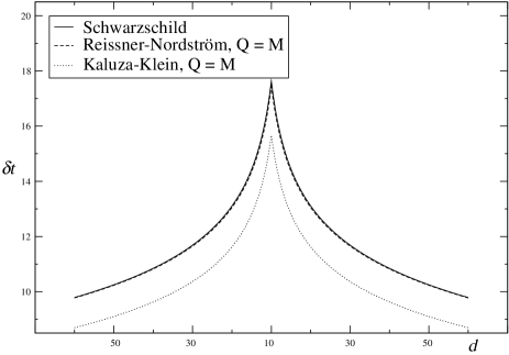
Figure 3: The time delay due to geometrical lensing as a function of the absolute value of the distance of closest approach of the light ray. As a light source moves behind the black hole, the arrival time of its radiation increases. Here, $d$ measures the absolute value of the distance of closest approach ($d=|r_{0}|$) and ranges from 50M to 10M and back again.

VI Discussion

Without a Birkhoff type theorem for higher dimensional black holes, the question of whether one might be able to determine the dimensionality of spacetime through gravitational light bending and time delay observations will clearly depend upon what one takes to be an appropriate black hole solution in higher dimensions. Many “black hole” solutions exist in higher dimensional theories but these are often associated with non vanishing effective energy-momentum tensors (for example in brane world scenarios) that are capable of providing solutions with black hole like characteristics in 4-dimensions. The solution studied here is a solution to the vacuum equations in 5-dimensions and in the spirit of the original Kaluza-Klein idea encodes the electromagnetic vector potential into the higher dimensional metric tensor.

In this work one is simply asking the question of whether or not one could in principle determine the difference between a 4-dimensional charged black hole where the source of the electric field is a residual charge and a 5-dimensional black hole where the electromagnetic potential seen in 4-dimensions is really an aspect of a higher-dimensional theory.

Table 1: Deflection angles, $\delta\phi$, additional path lengths, $c\delta t$, and time delays, $\delta t$, for a photon trajectory starting and finishing at $10^{5}M$ from the black hole and with a distance of closest approach of $r_{0}=10^{2}M$. Here the mass units are measured in terms of solar mass units where $M=Gm_{\odot}/c^{2}\approx 1.4748$ km.

	Schwarzschild	Reissner-Nordström		Kaluza-Klein
	$Q=0$	$Q=M/2$	$Q=M$	$Q=M/2$	$Q=M$
$\delta\phi$ (deg)	2.33641267	2.33303785	2.32291269	2.26473475	2.05205798
$c\delta t$ (km)	17.2313652	17.2227324	17.1968379	16.7431271	15.2800283
$\delta t$ (msec)	0.05743788	0.05740911	0.05732279	0.05581042	0.05093343

It has been shown in this work that if the black hole is of the charged Liu-Wesson type then one should be able to easily resolve the issue since the Kaluza-Klein black hole necessarily introduces effects at first order in both the bending angle and the time delay where the charge can makes itself known to the observer. While the charge might be determined by an independent measurement, one could in practice attempt to determine the bending angle, time delay and charge through measurements that would require a best fit through the data. This is what is usually done in gravitational lensing observations where the distance of closest approach or the impact parameter cannot be immediately determined without knowing the source position and the initial direction of the photons themselves.

In order to show how large these effects might be for astrophysical black holes, Table 1 is included in order to provide a comparison of the light bending angles and the Shapiro delays for black holes where $M$ equals one geometric solar mass unit. Geometric units are converted to the MKS system with the appropriate factors of $G$ and $c$ re-introduced. The distance of closest approach of the photon trajectory is set at $r_{0}=100M$ and the time delay is computed over a distance equal to $10^{5}M$. This is far enough from the black hole so that no changes to the value of the bending angle occur to an accuracy of one part in $10^{7}$. The bending angles are given in degrees while the effective path length that the photon must travel due to spacetime curvature and its associated time delay are given in kilometres and milliseconds respectively. As expected from the results shown in Figs. 2 and 3, even a significantly charged black hole of the Reissner-Nordstrom type makes only negligible changes to the light bending angles and time delays. On the other hand the charged Kaluza-Klein black hole will produce very noticeable changes in the measurements of such quantities.

Of course, the time delay measurements require that the light source has some known time dependent behaviour with a stable enough period that would allow one to compare the the differences in arrival time of signals from the source as it passes behind the black hole. Therefore one might take advantage of the lensing of a variable star or (better yet) a pulsar hkp in order to make measurements that would test the dimensionality of space-time.

- (1) J. Bodenner and C.M. Will, Am. J. Phys., 71, 770, (2003).
- (2) E.F. Eiroa, G.E. Romero and D.F. Torres, Phys. Rev. D 66, 024010 (2002).
- (3) M. Sereno, Phys. Rev. D 67 064007 (2003).
- (4) A. Bhadra, Phys. Rev. D 67, 103009 (2003).
- (5) V. Bozza, S. Capozziello, G. Iovane and G. Scarpetta, Gen. Rel. Grav., 33, 1535, (2001).
- (6) V. Bozza, Phys. Rev. D 66, 103001 (2002).
- (7) V. Bozza and L. Mancini, Gen. Rel. Grav., 36, 435, (2004).
- (8) S. Frittelli, T.P. Kling and E.T. Newman, Phys. Rev. D 61, 064021 (2000).
- (9) K.S. Virbhadra and G.F.R. Ellis, Phys. Rev. D 62, 084003 (2000).
- (10) B. Punsley, Ap. J., 498, 640 (1998).
- (11) H. Liu and P.S. Wesson, Class. Quan. Grav., 14, 1651 (1997).
- (12) A.S. Majumdar and N. Mukhurjee, Mod. Phys. Lett., A20, 2487, (2005).
- (13) E.F. Eiroa, Braz. J. Phys., 35, 1113, (2005).
- (14) E.F. Eiroa, Phys. Rev. D 71, 083010, (2005).
- (15) S. Weinberg, Gravitation and Cosmology, John Wiley and Sons, NY (1972)
- (16) D. Hobill, J. Kollar, and J. Pulwicki, in Short-Period Binary Stars: Observations, Analysis and Results, edited by E. Milone, D. Leahy and D. Hobill, (Springer, Dordrecht, 2007), p. 63.