Non-parametric Dark Energy Degeneracies

Abstract

We study the degeneracies between dark energy dynamics, dark matter and curvature using a non-parametric and non-perturbative approach. This allows us to examine the knock-on bias induced in the reconstructed dark energy equation of state, $w(z)$, when there is a bias in the cosmic curvature or dark matter content, without relying on any specific parameterisation of $w$. Even assuming perfect Hubble, distance and volume measurements, we show that for $z>1$, the bias in $w(z)$ is up to two orders of magnitude larger than the corresponding errors in $\Omega_{k}$ or $\Omega_{m}$. This highlights the importance of obtaining unbiased estimators of all cosmic parameters in the hunt for dark energy dynamics.

I Introduction

Since 1998 perlm ; riess evidence has been mounting in support of an accelerated expansion of the Universe. Nearly 10 years on, the puzzle of the origin of this acceleration – dubbed dark energy – remains one of the most intriguing enigmas in modern day science. Much activity has come from both the theoretical and observational sectors of the physics community in an attempt to pin down its origin. The current drive in dark energy studies is focused on trying to establish its dynamical behaviour as a function of redshift, $w(z)$. While the simplest explanation remains a $\Lambda$CDM universe with $w=-1$ for all redshift, dynamics in $w(z)$ would provide a window into new physics. Therefore, uncovering the dynamics of dark energy as described by the ratio of its pressure to density, $w(z)=p_{DE}/\rho_{DE}$, has become the focus of multi-billion dollar proposed experiments using a wide variety of methods, with several planned surveys at redshifts above unity, as high-redshift measurements are useful to constrain dark energy parameters and test for deviation from the concordance $\Lambda$CDM model (see e.g. DETF ). Unfortunately the search for dynamical behaviour in $w$ is a mani-fold problem. The nature of dark energy is elusive: cosmic observations depend not only on dark energy but also on other cosmic parameters such as the cosmic curvature, $\Omega_{k}$, and the total matter content, $\Omega_{m}$, leading to degeneracies between these and $w(z)$ parameters, an issue which has recently been under intense scrutiny by the community m1 ; CCB ; linder ; huang . Kunz m1 argues that observations are only sensitive to the full energy-momentum tensor and thus cannot see beyond a combination of the “dark component” – dark matter plus dark energy. The degeneracy between the geometry of the universe and the equation of state of dark energy has also been discussed in light of the well-known result that a cosmological constant in the presence of spatial curvature can mimic a dynamical dark energy CCB .

In this work we review current constraints on cosmic curvature and extend the approach in CCB in two ways. First we include the reconstruction of $w(z)$ that would follow from measurements of the rate of change of cosmic volume with redshift, $dV/dz$. Secondly we discuss the $w(z)$ that would be incorrectly reconstructed from perfect Hubble, distance and volume data if the wrong value of $\Omega_{m}$ were used. We assume perfect data for all observations, which allows us to probe fundamental, “in-principle” degeneracies that are not due to finite errors and incomplete redshift-coverage. This implies that given a specific bias in a cosmological parameter, the degeneracies will be true no matter what progress is made in improving future cosmic surveys. Furthermore, the key point in our reconstruction of $w(z)$ is that it is performed in a fully non-parametric manner, and so does not rely on the validity of any particular parameterisation of $w(z)$. To illustrate the power of this non-parametric approach, we compare our method with a standard equation of state parameterisation cp ; lin , which cannot fully resolve the above degeneracies.

I.1 Degeneracies in Dark Energy Studies

The success of the inflationary scenario for the early Universe and its standard prediction of flatness to high precision ($\Omega_{k}<10^{-10}$) is perhaps the main reason why curvature has traditionally been left out in analyses of dark energy. However, possible scenarios in which inflation is consistent with non-zero spatial curvature have recently been investigated freivogel . It is also interesting to note that the backreaction of cosmological fluctuations may cause effective non-zero curvature that may yield practical limits on our ability to measure $w(z)$ accurately at $z>1$ (see e.g. backreact ). Since measurements of the Cosmic Microwave Background (CMB) have so far proved consistent with flatness (e.g. wmap3 ) statistical quantities that measure the necessity of introducing extra parameters (such as Bayesian Evidence or information criteria BCK ; m2 ; trotta ) do not favour the inclusion of curvature as a parameter in current analyses liddle2 . However this is more a symptom of the inability of current data to constrain an extra parameter than a conclusive case for a flat universe. Further, Bayesian evidence or information criteria do not take into account the power of the biases that may be introduced by falsely neglecting a parameter. We will show below that the biases introduced in neglecting curvature are very significant at $z>1$.

In general constraints on curvature are very fragile to assumptions about the dark energy since they are primarily derived from distance measurements ($d_{L}$ or $d_{A}$) which are completely degenerate with curvature weinberg70 . One way to illustrate the degeneracy between curvature and dynamics is as follows. Let us assume that we know all cosmic parameters perfectly other than the curvature $\Omega_{k}$ and the dark energy equation of state, $w(z)$. At any redshift, $z_{*}$, a perfect measurement of $d_{L}(z_{*})$ (or $d_{A}(z_{*})$) allows us to measure a single quantity. If we know $w(z_{*})$ then that quantity can be $\Omega_{k}$. However, if $w(z)$ is truly a free function, then its value at $z_{*}$ is completely free and we are left trying to find two numbers from a single observation, which is impossible.

Only when we start to correlate the values of $w(z)$ at different redshifts can we begin to use distance measurements alone to constrain the curvature. The standard way to do this is to assume that $w(z)$ can be compressed onto a finite-dimensional subspace described by $n$ parameters, e.g.

$$w(z)=\Sigma_{j}^{n}w_{j}z^{j}$$ (1)

In this case perfect distance measurements at $n+1$ different redshifts will allow a complete solution of the problem and will yield the $w_{j}$ and $\Omega_{k}$. The most extreme version of this is to assume $\Lambda$CDM, $w(z)=-1$. Within this context it is of course possible to derive very stringent constraints on the curvature. For example, combining the WMAP 3 year data and the SDSS DR5 Luminous Red Galaxy (LRG) sample leads to $\Omega_{k}=-0.003\pm 0.010$ assuming $w=-1$ sdsslrg . The addition of extra data is crucial since the WMAP data alone provides only the constraint $\Omega_{k}=-0.3040+0.4067\Omega_{\Lambda}$ wmap3 .

It is a highly non-trivial statement that flat $\Lambda$CDM models provide such a good fit to all the data, but we must be aware that such constraints on the curvature are artificially strong in the sense that adding more dark energy parameters will lead to an almost perfect degeneracy with the curvature. This is visible in Fig. 17 of the WMAP3 wmap3 (here Fig. 1) which shows the correlation between a constant $w$ and $\Omega_{k}$.

Figure 1: The curvature-dark energy degeneracy Contours showing the 2D marginalized contours for $w$ and $\Omega_{k}$ based on combined data from WMAP3, 2dFGRS, SDSS and supernova surveys. While the slope of the degeneracy differs for this combination of data, the sign of the degeneracy is consistent with the $w_{0}$ term in Eqs. (IV),(IV). Taken from wmap3 .

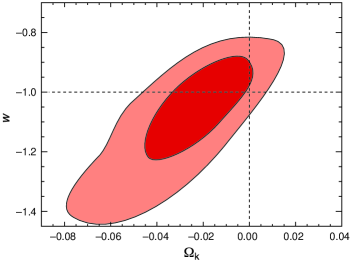
Hence we can currently say very little about the true value of the $\Omega_{k}$ and the belief that the spatial curvature is small is essentially based on Occam’s Razor. Although one could fit distance measurements with any value of $\Omega_{k}$, the required $w(z)$ functions would be disfavoured by Bayesian model selection which penalize models with extra parameters that do not significantly improve the fit. We show in detail later the required $w(z)$ functions to do precisely this.

At present a well-defined program for measuring the spatial curvature of the cosmos does not exist. To illustrate this, consider fixing the dark energy to be described by only $n$ parameters. One would hope that given this restriction the resulting constraints on $\Omega_{k}$ would be independent of the precise choice of the $n$ parameters, i.e. independent of the parameterisation. Unfortunately a little thought makes it clear that this cannot be true. A parameterisation of $w(z)$ which does not allow mimicry of curvature will provide good, decorrelated constraints on the curvature (which does not mean the corresponding best-fit will be a good fit to the data) while a model which allows perfect mimicry of the dynamics of the curvature (i.e. $(1+z)^{2}$) will show highly correlated constraints (although for negative $\Omega_{k}$ mimicry of distance data is only possible up to a critical redshift as we show later).

Figure 2: The curvature-dark energy degeneracy likelihood for $\Omega_{k}$ for different parameterisations of dark energy. Assuming a constant model for $w$, allows $\Omega_{k}$ to be tightly constrained at $2\sigma$ to be near 0. However introducing dynamics reduces these constraints significantly. Here $X(z)=\rho_{X}(z)/\rho_{X}(0)$ is the dark energy density, which wang assume is a free function below some cut-off redshift $z_{cut}$. The value of $X$ at redshifts $z_{i}=z_{cut}(i/n),i=1,2..,n$ are treated as $n$ independent model parameters that are estimated from the data. A specific functional form for $X$ is assumed above the cut-off redshift. The likelihoods are given for two such forms of $X(z)$; namely a power law, $X\propto(1+z)^{\alpha}$ for $z>z_{cut}$, and an exponential function $X\propto e^{\alpha z}$. In these figures there are $n=3$ independent redshifts below a cut-off redshift of $z_{cut}=1.4$. Taken from wang .

 

Figure 3: Left - $1\sigma$ error contours assuming flatness for the dark energy parameters $w_{0}$ and $w_{a}$ for the CPL parameterisations. Right - as on the left but with curvature left free and marginalised over. Note how pure distance measurements suffer strongly even with the very limited $w(z)$ parameterisation but that when all the surveys are combined the final error ellipse is essentially unaffected. This is to be expected from Equation (6) which shows how $\Omega_{k}$ can be determined from simultaneous Hubble rate and distance measurements. Figure from Knox et al. knox .

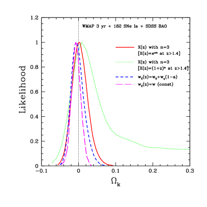
This dilemma is visible in various recent studies attempting to constrain cosmic curvature in the presence of multiple dark energy $w(z)$ parameters groupbb ; wang ; huang . For some popular parameterisation constraints on $\Omega_{k}$ are of order $|\Omega_{k}|<0.05$ at $2\sigma$. For other parameterisation the constraints evaporate and even $\Omega_{k}\sim 0.2$ cannot be ruled out (see Fig. 2, which is taken from wang ).

Alternative cosmic measurements sensitive to curvature include the Integrated Sachs Wolfe (ISW) effect, which is sensitive to the growth of the metric fluctuations $\Phi$, which is in turn sensitive to both dark energy and curvature. Recent work to investigate the ISW effect as a function of redshift uses the combination of CMB data with information on large scale structure isw . Combining WMAP with such suitable tracers of large scale structure shows that $\Phi$ has been decreasing with cosmic time nolte , which rules out a large positive curvature which would have predicted the opposite trend.

Another measurement sensitive to the growth function is differential number counts $dN/dz$, e.g. of clusters. This is a potentially sensitive test which, given a constant comoving number of objects, reduces to a test of the rate of change of cosmic volume with redshift, $dV/dz$. We discuss in detail below how perfect measurements of $dV/dz$ allow reconstruction of $w(z)$, and we discuss the resulting errors on dark energy when systematic biases in cosmic parameters are present.

Measurements of the power spectrum from CMB data and from measurement of Baryon Acoustic Oscillations (BAO) provide estimates of the matter content of the universe. While constraints on $\Omega_{m}$ are sharpened by combining data from many observations, the best-fit value is often derived on the assumption of flatness sdsslrg ; perciv . Unlike the case for cosmic curvature the degeneracy between observables and the matter content is perfect and we show that incorrectly assuming a particular value for $\Omega_{m}$ can also mimic deviations from $\Lambda$CDM.

I.2 Future surveys

We will show in equation (6) that simultaneous measurements of the Hubble rate $H(z)$, distance $D\propto d_{A},d_{L}$ and $D^{\prime}(z)$ allow for a perfect measurement of $\Omega_{k}$. BAO allow for the simultaneous measurement of both distance and Hubble rate at the central redshift bao . For a flat universe $D^{\prime}(z)\propto 1/H(z)$, but in a curved universe this is not true: the curved geodesics mean that $D^{\prime}(z)$ contains extra information encoded in $\Omega_{k}$.

Measuring $D^{\prime}(z)$ is in principle possible with future BAO, weak lensing and supernova surveys. In particular, cross-correlation tomography of deep lensing surveys appears to be a very powerful probe of curvature when combined with BAO surveys bernstein , assuming that self-calibration is possible. In principle it should be possible to measure the cosmic curvature to an accuracy of about $\sigma(\Omega_{k})\simeq 0.01$ for an all-sky weak lensing and BAO survey out to $z=10$. In principle such a survey would be able to measure distances to about $10^{-4}f_{sky}^{-1/2}$ in redshift bins of width $\Delta z=0.1$ out to $z=2.5$ bernstein . 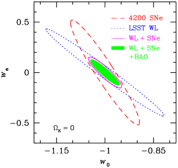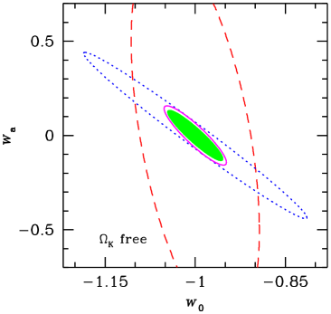This relies critically on the combination of weak lensing and BAO data since constraints from either observations alone are significantly degraded. This can also be seen in Fig. (3) which shows the error ellipses for the parameters in the CPL parameterisation $w(z)=w_{0}+w_{a}\left(\frac{z}{1+z}\right)$ assuming flatness (left) and leaving $\Omega_{k}$ free (right). Note that although individual error ellipses are significantly degraded, the combined data sets have an almost unchanged error ellipse.

Our work is organized as follows: we illustrate the dependence of the background observables on the cosmological parameters $\Omega_{m},\Omega_{k}$ in section II.1 and discuss obtaining the dark energy equation of state $w$ from observables in section II.2. The process of reconstructing $w$ via a non-parametric approach is described in section III. Finally we link this non-parametric approach to other standard approaches to dark energy degeneracies in section IV and conclude in section V.

II Dark Energy from observations

There are three key observables of the background geometry which play a pivotal role in determining $w(z)$, namely measurements of distances, of the expansion history (i.e. the Hubble parameter) and of the change in the fractional volume of the Universe (e.g. from number-counts).

The principle method to date is to relate measurements of the distances of objects to the cosmology of the Universe. This is done via either standard ‘rulers’ of known length - giving the angular diameter distance $d_{A}(z)$ - or via standard ‘candles’ of known brightness which results in the luminosity distance $d_{L}(z)$. These are related via the reciprocity relation $d_{L}(z)=(1+z)^{2}d_{A}$. In an FLRW model, these are given by $d_{L}(z)=c(1+z)D(z)/H_{0}$, where we define

$$D(z)=\frac{1}{\sqrt{-\Omega_{k}}}\sin{\left(\sqrt{-\Omega_{k}}\int_{0}^{z}{\mathrm{d}z^{\prime}\frac{H_{0}}{H(z^{\prime})}}\right)}.$$ (2)

Here, $\Omega_{k}$ is the usual curvature parameter, and $H(z)$ is given by the Friedmann equation,

$$H(z)^{2}=H_{0}^{2}\left[\Omega_{m}(1+z)^{3}+\Omega_{k}(1+z)^{2}+\Omega_{\mathrm{D}E}f(z)\right]$$ (3)

where

$$f(z)=\exp{\left[3\int_{0}^{z}\frac{1+w(z^{\prime})}{1+z^{\prime}}\mathrm{d}z^{\prime}\right]}$$ (4)

and $\Omega_{DE}=1-\Omega_{m}-\Omega_{k}$. Thus, given a cosmological model, we may calculate any distance measure we choose.

The Hubble parameter is in itself an observable which will play an important role in future dark energy experiments. Knowledge of $H(z)$ allows us to directly probe the dynamical behavior of the universe, and it will be directly determined from BAO surveys which simultaneously provide the angular diameter distance, $d_{A}$ at the same redshift by exploiting the radial and angular views of the acoustic oscillation scale bao , a fact that will provide key new data in coming years sdsslrg ; wfmos ; wigglez .

The third key background test we will discuss here is the observation of fractional volume change as a function of redshift,

$${V}^{\prime}(z)\equiv\frac{\mathrm{d}^{2}V}{\mathrm{d}z\mathrm{d}\Omega}=\frac{c^{3}D(z)^{2}}{H_{0}^{2}H(z)},$$ (5)

which can in principle be determined via number-counts or the BAO.

Given any two of the above observables we may deduce the third. Perfect observations of these observables should allow us, in principle, to be able to reconstruct two free functions when in fact we only need to reconstruct one, namely $w(z)$, as well as two cosmological parameters, $\Omega_{m}$ and $\Omega_{k}$. (Note that if we know $H(z)$ perfectly, we know $H_{0}=H(0)$, and so this is no longer a free parameter in the same sense.) How do we find these?

We may determine the curvature directly, and independently of the other parameters or dark energy model via the relation CCB

$$\Omega_{k}=\frac{\left[H(z)D^{\prime}(z)\right]^{2}-H_{0}^{2}}{[H_{0}D(z)]^{2}},$$ (6)

which may be derived directly from Eq. (2). Such independent measurements of the curvature of the universe can in turn be used to test the Copernican Principle in a model-independent way. copernican

II.1 Expansions of the background observables

To illustrate the dependency of the background observables we consider here we expand them in terms of the cosmological parameters $\epsilon_{m}$, $\Omega_{k}$ and the parameter $x=z/(1+z)$. Here $\epsilon_{m}:=\Omega_{m*}-\Omega_{m}$, where $\Omega_{m*}$ is the true value of the matter energy density and $\Omega_{m}$ is the assumed value, as seen in Eq. (III.2).

The expansions for $H(x),d_{L}(x),V^{\prime}(x)$ yield

$$x=\frac{z}{1+z}$$

$$H(x)=H_{0}\bigg{[}1+\frac{1}{2}\big{\{}3(1+w_{0}(1-\Omega_{m*}))x-(1+3w_{0})\Omega_{k}x-3w_{0}\epsilon_{m}\big{\}}\bigg{]}$$ (7)

$$d_{L}(x)=\frac{cx}{H_{0}}\bigg{[}1+\big{\{}(5+3w_{0}(\Omega_{m*}-1))+(1+3w_{0})\Omega_{k}+3w_{0}\epsilon_{m}\big{\}}x\bigg{]}$$ (8)

$$V^{\prime}(x)=\frac{c^{3}x^{2}}{H_{0}^{3}}\bigg{[}1+\big{\{}(-1+3w_{0}(\Omega_{m*}-1))+(1+3w_{0})\Omega_{k}+3w_{0}\epsilon_{m}\big{\}}x\bigg{]}$$ (9)

It can be seen from equations (7, 8, 9) that the leading term corresponds to that of the standard flat $\Lambda$CDM model. From these equations we can directly compute the error on the particular observable as a function of redshift based on the difference between the ‘true’ cosmology and the ‘assumed’ cosmological model.

II.2 Obtaining the Dark Energy equation of state from Observations

Assuming we have ‘perfect’ and uncorrelated data from observations we would like to reconstruct $w(z)$ without assuming a specific parameterisation. Depending on the particular observable of interest, there are different ways to reconstruct $w$.

Dark energy from Hubble

It is straightforward to find $w(z)$ from the Hubble rate huterer_hzw ; linder , from Eq. (3), and is given by:

$$w(z)=-\frac{1}{3}\frac{\Omega_{k}H_{0}^{2}(1+z)^{2}+2(1+z)HH^{\prime}-3H^{2}}{H_{0}^{2}(1+z)^{2}[\Omega_{m}(1+z)+\Omega_{k}]-H^{2}}.$$ (10)

This tells us $w(z)$ provided we already know $\Omega_{m}$ and $\Omega_{k}$. However, this reveals a degeneracy between $\Omega_{m}$ and $w(z)$ which cannot be overcome by background tests alone m1 . In essence, geometric background tests can measure the combination $\Omega_{m}+\Omega_{DE}f(z)/(1+z)^{3}$, but not the two separately. Another way to view this is by differentiating Eq. (10), and eliminating $\Omega_{m}$ to give a differential equation for $w(z)$ in terms of $H,H^{\prime}$ and $H^{\prime\prime}$; the constant arising in the general solution to this differential equation is $\Omega_{m}$.

Similarly, we can reconstruct $w(z)$ from the other two tests on their own.

Dark energy from distance measurements

From distance measurements, we may invert Eq. (2) to find

$$w\left(z\right)={\frac{2\,\left(1+z\right)\left(D^{2}\Omega_{{k}}+1\right){D}^{\prime\prime}-{D}^{\prime}\left[\Omega_{{k}}\left(1+z\right)^{2}{D}^{\prime 2}+2\,\Omega_{{k}}{D}\left(1+z\right){D}^{\prime}-3-3\,{D}^{2}\Omega_{{k}}\right]}{3\left\{\left[\Omega_{{k}}+\Omega_{{m}}\left(1+z\right)\right]\left(1+z\right)^{2}D^{\prime 2}-D^{2}\Omega_{{k}}-1\right\}{D}^{\prime}}}.$$ (11)

Reconstructing $w(z)$ from volume measurements as an analytical formula is rather tricky (as it involves the root of a quartic power). It is simpler instead to reconstruct $w(z)$ by solving the differential equation for $f(z)$ and then differentiating to get $w(z)$.

Dark energy from volume measurements

Starting with Eq. (2), we solve for the derivative of the Hubble parameter and equate this with the expression for $H^{\prime}$ in terms of $w(z)$ from Eq. (10) and use

$$w(z)=\frac{(1+z)f^{\prime}}{3f}-1$$ (12)

to yield a first order differential equation for $f$, namely

$$f^{\prime}(z)=\frac{A(z)+B(z)+C(z)}{-H_{0}^{2}V^{\prime}\Omega_{\mathrm{DE}}},$$ (13)

where

$$A(z)=-4{\left(V^{\prime}H_{0}\left(c^{3}\sqrt{f(z)\Omega_{\mathrm{DE}}+X_{11}}+V^{\prime}H_{0}^{3}\Omega_{k}\left(f(z)\Omega_{\mathrm{DE}}+X_{11}\right)\right)\right)}^{1/2},$$

with

$$X_{ab}=(1+z)^{2}(a\Omega_{k}+b\Omega_{m}(1+z)),$$

$$B(z)=2H_{0}^{2}V^{\prime\prime}\left(f(z)\Omega_{\mathrm{DE}}+X_{11}\right)$$

and

$$C(z)=H_{0}^{2}V^{\prime\prime}\frac{X_{32}}{1+z}.$$

We solve this for $f(z)$ and then use (12) again to yield $w(z)$. The solution for $f(z)$ is unique since we demand $f(0)=1$.

III Reconstructing $w(z)$

If we knew $\Omega_{m}$ and $\Omega_{k}$ perfectly then our three expressions for $w(z)$ would yield the same function $w(z)$, assuming we lived in an exact FLRW universe. But what if – as is commonly assumed – we impose $\Omega_{k}=0$ when in fact the true curvature is actually non-zero? It is usually implicitly assumed that the error on $w(z)$ will be of order $\Omega_{k}$, but, as was shown in CCB this is not the case. Will measuring $V^{\prime}(z)$ possibly circumvent this? And furthermore, are there similar issues from an imperfect knowledge of $\Omega_{m}$?

Figure 4: Reconstructing the dark energy equation of state assuming zero curvature when the true curvature is 2% in a closed $\Lambda$CDM universe. The $w(z)$ reconstructed from $H(z)$ is phantom ($w<-1$) and rapidly acquires an error of order 50% and more at redshift $z\gtrsim 2$, and diverges at finite redshift. The reconstructed $w(z)$ from $d_{L}(z)$ for $\Omega_{k}<0$ is phantom until $z\approx 0.86$, where it crosses the true value of $-1$ and then crosses 0 at high redshift, where the bending of geodesics takes over from dynamical behavior, producing errors in opposite direction to the DE reconstructed from $H(z)$. In order to make up for the missing curvature, the reconstructed dark energy is behaving like a scalar field with a tracking behavior. These effects arise even if the curvature is extremely small $(<0.1\%)$. Reprinted from CCB .

III.1 Zero curvature assumption

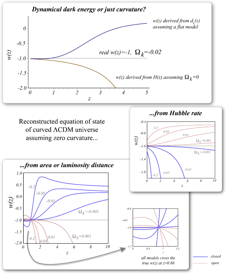
We can easily see the implications of incorrectly assuming flatness by constructing the functions $d_{L}(z)$ and $H(z)$ under the assumption of the $\Lambda$CDM in a curved Universe (i.e. assuming $w=-1,\Omega_{k}\neq 0$) and inserting the results into Eqs (10) and (11).

If we then set $\Omega_{k}=0$ in Eqs. (10) and (11) we arrive at the two corresponding $w(z)$ functions (if they exist) required to reproduce the curved forms for $H(z)$ and $d_{L}(z)$ in a flat Universe with dynamic dark energy. This would apply equally to $d_{A}(z)$ for that matter - the results are exactly the same for any distance indicator. Figure 4 presents this method using for simplicity the concordance value of $w=-1$ but we have checked that the qualitative results do not depend on the ‘true’ underlying dark energy model . We assume $\Omega_{m}=0.3$ in all expressions; numbers quoted are weakly dependent on this. The resulting (spurious) $w(z)$ can then be thought of as the function required to yield the same $H(z)$ or $d_{L}(z)$ as in the actual curved $\Lambda$CDM model: e.g.,

$$d_{L}[\text{flat},w(z)]=d_{L}[\text{curved},w(z)=-1].$$ (14)

For example for the Hubble rate the reconstructed $w(z)$ can be found analytically to be

$$w(z)=-\frac{1}{3}\frac{\Omega_{k}(1+z)^{2}+3\Omega_{\mathrm{DE}}}{\Omega_{k}(1+z)^{2}+\Omega_{\mathrm{DE}}},$$ (15)

without any dependence on a specific parameterisation.

In the figure we show what happens for $\Lambda$CDM: curvature manifests itself as evolving dark energy. In the case of the Hubble rate measurements this is fairly obvious - we are essentially solving the equation $\Omega_{DE}f(z)=\Omega_{\Lambda}+\Omega_{k}(1+z)^{2}$ where $f(z)$ is given by Eq. (4). For $\Omega_{k}>0$, $w(z)$ must converge to $-1/3$ to compensate for the curvature. For $\Omega_{k}<0$, the opposite occurs and a redshift is reached when $w\rightarrow-\infty$ in an attempt to compensate albeit unsuccessfully for the positive curvature. Already we can see why the assumption that the error in $w$ is of order the error in $\Omega_{k}$ breaks down so drastically.

Interestingly, the curved geodesics imply that the error in $w$ reconstructed from $d_{L}(z)$ and $H(z)$ have opposing signs at $z\gtrsim 0.9$, as can be seen by comparing the panels for the Hubble rate and the distance indicator in Fig. 4. Above the critical redshift the effect of curvature on the geodesics becomes more important than the pure dynamics, and the luminosity distance flips $w(z)$ in the opposite direction to that reconstructed from $H(z)$.

In the case of volume measurements the reconstructed $w(z)$ has a similar form to the $w$ we obtained from the distance measurements $D(z)$. This can be seen from Eq. (5), where the distance information enters the equation as a square power. For example in the closed Universe case the reconstructed $w(z)$ drops to more phantom values ($-2.5$ compared to $-1.3$ for the distance measurements) in order to make up for the missing curvature.

Again the effect of curvature on the geodesics dominates the effect of dynamics for large $z$, and the distance contribution in the volume measurements flips the reconstructed $w(z)$ at $z=1.6$. The critical redshift of this flip is determined by the redshift at which the curvature of the geodesics affecting distance measurements becomes more important than the expansion rate. This playoff becomes more finely balanced for volume measurements due to the fact that $H(z)$ appears both in $D(z)$ (as a square power) and on its own. Hence $w(z)$ has to work harder in reproducing curvature to counterbalance the opposing trends of expansion history and geometry, and so the balance is achieved at higher redshift. The specific redshift at which this happens is dependent on $\Omega_{m}$ in that lower values imply higher value of the critical redshift.

Figure 5: Reconstructed dark energy from volume measurements while incorrectly assuming flatness - Similar to the case for distance measurements in a closed Universe, the reconstructed $w(z)$ must initially be phantom in order to compensate for curvature, and crosses the true value of $w=-1$ at a redshift of $z~{}1.6$, which is greater than the redshift of 0.86 for the distance measurements alone CCB . After this point, the $w(z)$ increases to overcome the curvature of the geodesics.

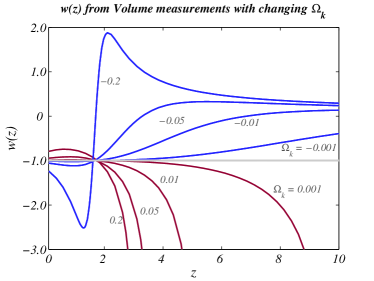
We have shown that incorrectly assuming flatness can result in a reconstructed $w(z)$ that mimics dynamics, yielding errors on $w$ that are much larger than the order of errors on $\Omega_{k}$. One might then ask if similar errors will result when incorrectly assuming a particular value for the matter density in the Universe, $\Omega_{m}$.

III.2 Uncertainties in the Matter content $\Omega_{m}$

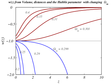
We consider the similar case of reconstructing $w(z)$ in a flat Universe but here the errors occur when assuming the concordance value of $\Omega_{m}=0.3$ incorrectly. For example in this case the $w(z)$ reconstructed from Hubble measurements Eq. (10) reduces to

$$w(z)=-\frac{1}{3}\frac{2(1+z)HH^{\prime}-3H^{2}}{H_{0}^{2}(1+z)^{2}[\Omega_{m}(1+z)]-H^{2}}.$$ (16)

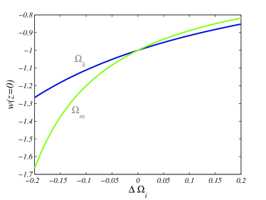
Similar expressions are found for both the distance and volume measurements. The $w(z)$ curves obtained from incorrectly assuming $\Omega_{m}=0.3$ are shown in Fig. 6. If we assume flatness for this example we find that changing the value of $\Omega_{m}$ can only affect the dark energy density, and thus change the value of $H(z)$. As $\Omega_{m}$ is only present in all three observables through $H(z)$ or integrals of $1/H(z)$, the reconstructed $w(z)$ is the same for all three measurements. Interestingly, the reconstructed $w(z)$ curves do not go through $w=-1$ at $z=0$, but are spread between -0.85 and -1.15 for $0.2<\Omega_{m}<0.4$. This is also shown in Fig. 7.

Figure 6: Reconstructed dark energy from an incorrectly estimated matter density - The reconstructed $w(z)$ for changing $\Omega_{m}$ from all three measurements ($H,D,dV/dz$). Since we assume flatness while changing $\Omega_{m}$, all three observables yield the same reconstructed $w(z)$, since $\Omega_{m}$ only enters the functions through $H(z)$ or integrals of $1/H$. For $\Omega_{m}>0.3$ the dark energy tries to compensate for the extra matter contribution and so asymptotes to $w=0$ as $z\rightarrow\infty$. For $\Omega_{m}<0.3$ the $w(z)$ is of the same form to what is reconstructed from neglecting curvature in a closed Universe (see Fig. 4), and the phantom $w$ tends to $-\infty$ as it attempts to compensate for the ‘missing’ matter density.

Given any scenario of an assumed cosmology that differs from the ‘true’ Universe, we can derive the value of today, $w(z=0)$ from both the Hubble and distance measurements as

$$w(0) = \frac{3-4\Omega_{k*}-3\Omega_{m}+\Omega_{k}}{6\Omega_{m}+6\Omega_{k*}-3\Omega_{m*}-3-3\Omega_{k}}$$

$$\sim \frac{\epsilon_{m}}{(-1+\Omega_{m*})}-\frac{2\Omega_{k}}{3(-1+\Omega_{m*})}-1,$$

where $\epsilon_{m}=\Omega_{m*}-\Omega_{m}$ as defined above where the asterisk indicates assumed but incorrect values of the corresponding quantities. We vary this equation in one ‘true’ density ($\Omega_{m}$ or $\Omega_{k}$) at a time, while keeping the other constant at the assumed value of either $\Omega_{k}=\Omega_{k*}$ or $\Omega_{m}=\Omega_{m*}$ to produce the curves in Fig. 7. This parameter $w(z=0)$ allows us to easily quantify the affect of assuming an incorrect cosmological model on the inferred low-redshift value of $w$.

Figure 7: Low redshift variation in $w(z)$ from $H(z)$ and $D(z)$- incorrectly assuming concordance values of $\Omega_{m}=0.3$ and $\Omega_{k}=0$ results in a variation in the low-redshift value of $w(z)$ reconstructed from observables. The relationship between the error in the cosmological parameter and the reconstructed value for $w$ (while keeping the other cosmological parameter fixed at the prior value) is shown for both $\Omega_{m}$ (the green curve) and $\Omega_{k}$ (the blue curve).

IV Parametric Degeneracies

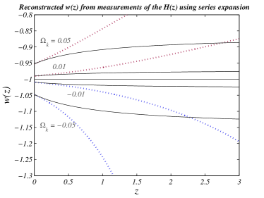
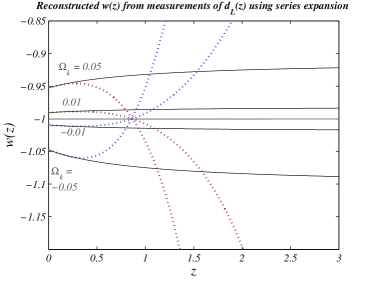
We now want to connect the non-parametric approach we have followed above with standard approaches to degeneracies and so we expand Eqs. (10) and (11) for the Hubble rate and distance measurements to first order in $x=z/(1+z)$. This allows us to link to the parameters $w_{0},w_{a}$ used in the Chevallier-Polarski-Linder (CPL) cp ; lin parameterisation $w_{\mathrm{CPL}}(z)=w_{0}+w_{a}\left(\frac{z}{1+z}\right)$, which is used in the Dark Energy Task Force report DETF . The values of $w_{0},w_{a}$ obtained using this expansion are given below.

From Hubble rate measurements

$$w_{0} = -\frac{\Omega_{k}+3\Omega_{\mathrm{DE}}}{3(1-\Omega_{m})}$$

$$w_{a} = \frac{4}{3}\frac{\Omega_{k}\Omega_{\mathrm{DE}}}{(1-\Omega_{m})^{2}}$$ (18)

From luminosity distance measurements

$$w_{0} = -\frac{\Omega_{k}+3\Omega_{\mathrm{DE}}}{3(1-\Omega_{m})}$$

$$w_{a} = -\frac{2}{3}\frac{\Omega_{k}(\Omega_{k}-\Omega_{\mathrm{DE}})}{(1-\Omega_{m})^{2}}$$ (19)

We plot in Figure 8 the non-parametric reconstructed $w(z)$ along with the reconstructed $w_{\mathrm{C}PL}(z)$ from the coefficients given by Eqs. (IV, IV) for the observables $H(z)$ and $d_{L}(z)$.

Figure 8: Degeneracies in standard parameterisations - $w(z)=w_{0}+w_{a}\frac{z}{1+z}$ using the coefficients in Eqs. (IV) and (IV) (solid lines) compared with the fully non-parametric $w(z)$ inferred from Hubble and distance measurements. Using a limited parameterisation of $w(z)$ like this incorrectly makes it appear that dark energy and curvature are not completely degenerate, leading to artificially strong constraints on curvature and $w_{0},w_{a}$.

V Conclusions and Outlook

We have explored the degeneracies between the dark energy equation of state $w(z)$ and cosmic parameters using a non-parametric approach. This means we are able to write down the precise $w(z)$ that will be reconstructed from perfect data if slightly wrong or biased values for the cosmic parameters $\Omega_{k},\Omega_{m}$ are assumed. This is complementary to traditional methods which typically use an aggressive compression of the $w(z)$ function onto a couple of parameters (usually $w_{0},w_{a}$) and then study the degeneracy between these and other cosmic parameters. Our approach is superior in one way however: degeneracies between $w(z)$ and some cosmic parameters such as $\Omega_{k}$ can appear to be quite weak in the parameterised approach. However, in the case of distance measurements this is completely artificial and due to strong assumptions about the allowed form of $w(z)$ since the degeneracy is perfect if $w(z)$ is allowed to be totally free.

We extend the work of CCB to show the reconstructed $w(z)$ from measurements of volume for both wrongly assumed $\Omega_{k}$ and $\Omega_{m}$. As with Hubble and distance measurements we show that the errors in $w(z)$ that result from uncertainty in the cosmic parameters are much larger than the uncertainty in $\Omega_{k}$ or $\Omega_{m}$, especially at large redshifts. We have shown that curvature affects measurements of $H(z)$ and $D(z)$ in complementary ways, with the error at high redshift having opposite signs for an error in $\Omega_{k}$. In the case of an $\Omega_{m}$ error, Hubble, distance and volume measurements all lead to the same erroneously reconstructed $w(z)$, a manifestation of the dark matter-dark energy degeneracy highlighted in m1 .

In this review we have assumed perfect data for Hubble rate, distance and volume at all redshifts. It would be interesting to extend our non-parametric approach to the case of imperfect data which has incomplete redshift coverage and errors on the observables. This is left to future work but will allow contact with the approaches in arman ; pilar .

Acknowledgments – we thank Luca Amendola, Chris Blake, Thomas Buchert, Daniel Eisenstein, George Ellis, Martin Kunz, Roy Maartens, Bob Nichol and David Parkinson for useful comments and insights. MC thanks Andrew Liddle and FTC for support. BB and CC acknowledge support from the NRF and RH acknowledges funding from KAT.

References

- (1) A. Albrecht et al., Report of the Dark Energy Task Force, astro-ph/0609591 (2006)
- (2) E. V. Linder, Astropart.Phys. 24, 391 (2005)
- (3) M. Kunz, astro-ph/0702615, (2007)
- (4) K. Glazebrook and the WFMOS Feasibility Study Dark Energy Team, White paper submitted to the Dark Energy Task Force, astro-ph/0507457; B. A. Bassett, R. C. Nichol and D. J. Eisenstein [for the WFMOS Collaboration], astro-ph/0510272;
-
(5)
See e.g. T. Buchert, M. Carfora, Phys. Rev. Lett. 90, 031101 (2003);
N. Li, D. J. Schwarz, gr-qc/0702043;
S. Rasanen, Class. Quant. Grav. 23 (2006) 1823;
A.A. Coley, N. Pelavas Phys. Rev. D75, 043506 (2007) - (6) See eg. T. Giannantonio et al., Phys. Rev. D 74, 063520 (2006); S. Ho et al. arXiv:0801.0642 801 (2008)
- (7) G. Bernstein, A. J. 637 (2006) 598
- (8) L. Knox, Y-S. Song, H. Zhan, astro-ph/0605536 (2006)
- (9) M. Tegmark et al., Phys. Rev. D 74, 123507 (2006)
- (10) K. Glazebrook et al., astro-ph/0701876 2007
- (11) D. Huterer & M. S. Turner, Phys. Rev. D 64, 123527 2001
- (12) S. Weinberg, ApJL 161, L233 (1970)
- (13) C. Clarkson, M. Cortês, & B. Bassett, J. C. A. P. 8, 11 (2007)
(14)
Y. Gong, Q. Wu & A. Wang, arXiv:0708.1817 (2007);
L. Mersini-Houghton, Y. Wang, P. Mukherjee &
E. Kafexhiu, arXiv:0705.0332 (2007); E. Wright, A. J. 664, 633 (2007); K. Ichikawa, M. Kawasaki, T. Sekiguchi, & T. Takahashi, J. C. A. P. 12, 5 (2006); C.-B. Zhao,
J.-Q. Xia, H. Li, et al., Phys. Lett. B, 648, 8 (2007);
K. Ichikawa, & T. Takahashi, , J. C. A. P. , 2, 1 (2007) - (15) Y. Wang & P. Mukherjee, astro-ph/0703780 (2007)
- (16) Z.-Y. Huang, B. Wang, & R.-K. Su, Int. Journ. Mod. Phys. A, 22, 1819 (2007)
- (17) D. N. Spergel et al. Ap. J. S. , 170, 377 (2007)
- (18) S. Perlmutter, et al. Ap. J. 483, 565 (1997)
- (19) A. G. Riess et al. A. J. , 116, 1009 (1998)
- (20) B. Freivogel, M. Kleban, M. Rodríguez Martínez, & L. Susskind, Journal of High Energy Physics, 3, 39 (2006)
- (21) M. Kunz, R. Trotta, & D. R. Parkinson, Phys. Rev. D 74, 023503 (2006)
- (22) R. Trotta, M. N. R. A. S. 378, 72 (2007)
- (23) A. R. Liddle astro-ph/0701113 (2007)
- (24) H. -J. Seo, & D. J. Eisenstein, Ap. J. , 598, 720 (2003); C. Blake, & K. Glazebrook, Ap. J. 594, 665 (2003)
- (25) M. Chevallier & D. Polarski Int. J. Mod. Phys. D 10, 213 (2001)
- (26) E. Linder P. R. L. 90, 091301 (2003)
- (27) W. J., Percival, et al. Ap. J. 657, 51 (2007)
- (28) B. A. Bassett, P. S. Corasaniti & M. Kunz, Ap. J. L. , 617, L1 (2004)
- (29) C. Espana-Bonet & P. Ruiz-Lapuente hep-ph/0503210 (2005)
- (30) A. Shafieloo, U. Alam, V. Sahni, V. & A. A. Starobinsky, M. N. R. A. S. 366, 1081 (2006)
- (31) A. Aguirre, C. P. Burgess, A. Friedland, & Nolte, D. Classical and Quant Gravity 18, 223 (2001)
- (32) C. Clarkson, B. A. Bassett, & T. Hui-Ching Lu, arXiv:0712.3457, 712 (2007)