Estimating the Redshift Distribution of Faint Galaxy Samples

Abstract

We present an empirical method for estimating the underlying redshift distribution $N(z)$ of galaxy photometric samples from photometric observables. The method does not rely on photometric redshift (photo-z) estimates for individual galaxies, which typically suffer from biases. Instead, it assigns weights to galaxies in a spectroscopic subsample such that the weighted distributions of photometric observables (e.g., multi-band magnitudes) match the corresponding distributions for the photometric sample. The weights are estimated using a nearest-neighbor technique that ensures stability in sparsely populated regions of color-magnitude space. The derived weights are then summed in redshift bins to create the redshift distribution. We apply this weighting technique to data from the Sloan Digital Sky Survey as well as to mock catalogs for the Dark Energy Survey, and compare the results to those from the estimation of photo-z’s derived by a neural network algorithm. We find that the weighting method accurately recovers the underlying redshift distribution, typically better than the photo-z reconstruction, provided the spectroscopic subsample spans the range of photometric observables covered by the photometric sample.

1 Introduction

On-going, wide-field surveys are delivering photometric galaxy samples of unprecedented scale. Optical and near-infrared surveys planned for the next decade will increase the sizes of such samples by an order of magnitude. Much of the utility of these samples for astronomical and cosmological studies rests on knowledge of the redshift distributions of the galaxies they contain. For example, surveys aimed at probing dark energy via clusters, weak lensing, and baryon acoustic oscillations (BAO) will rely on the ability to coarsely bin galaxies by redshift, enabling approximate distance-redshift measurements as well as study of the growth of density perturbations. The power of these surveys to constrain cosmological parameters will be limited in part by the accuracy with which the galaxy redshift distributions can be determined (Huterer et al., 2004, 2006; Zhan & Knox, 2006; Zhan, 2006; Ma et al., 2006; Lima & Hu, 2007).

Photometric redshifts (photo-z’s, denoted $z_{\rm phot}$ below) – approximate estimates of galaxy redshifts based on their broad-band photometric observables, e.g., magnitudes or colors – offer one technique for approaching this problem. Photo-z’s have the advantage that they provide redshift estimates for each galaxy in a photometric catalog; such information is useful for certain studies (Mandelbaum et al., 2007). However, in many applications we do not need such galaxy-by-galaxy information – instead, we only require an estimate of the redshift distribution of a sample of galaxies selected by some set of photometric observables. For example, cosmic shear weak lensing or angular BAO measurements rely on relatively coarse binning of galaxies in redshift, and it suffices to have an accurate estimate of the redshift distribution $N(z)$ for galaxies satisfying certain color or magnitude selection criteria (Sheldon et al., 2004, 2007a; Jain et al., 2007). Photo-z estimators are not typically designed to provide unbiased estimates of the redshift distribution: $N(z_{\rm phot})$ is biased by photo-z errors.

Although deconvolution (Padmanabhan et al., 2005) or other techniques (Sheth, 2007) can be used to obtain improved estimates of the redshift distribution from photo-z measurements, this problem motivates the development of a method optimized to directly estimate the underlying redshift distribution $N(z)$ for a photometric sample. In addition to its direct utility, a precise, unbiased estimate of the redshift distribution is useful even for probes that do require individual galaxy redshifts, since it provides a template for characterizing photo-z errors.

In this paper we present an empirical technique to estimate $N(z)$ for a photometric galaxy sample that is based upon matching the distributions of photometric observables of a spectroscopic subsample to those of the photometric sample. The method assigns weights to galaxies in the spectroscopic subsample (hereafter denoted the training set, in analogy with machine-learning methods of photo-z estimation), so that the weighted distributions of observables for these galaxies match those of the photometric sample. The weight for each training-set galaxy is computed by comparing the local “density” of training-set galaxies in the multi-dimensional space of photometric observables to the density of the photometric sample in the same region. We estimate the densities using a nearest neighbor approach that ensures the density estimate is both local and stable in sparsely occupied regions of the space. The use of the nearest neighbors ensures optimal binning of the data, which minimizes the requisite size of the spectroscopic sample. After the training-set galaxy weights are derived, we sum them in redshift bins to estimate the redshift distribution.

As we will show, this method provides a precise and nearly unbiased estimate of the underlying redshift distribution for a photometric sample and does not require photo-z estimates for individual galaxies. Moreover, the spectroscopic training set does not have to be representative of the photometric sample, in its distributions of magnitudes, colors, or redshift, for the method to work. We only require that the spectroscopic training set cover, even sparsely, the range of photometric observables spanned by the photometric sample. The method can be applied to different combinations of photometric observables that correlate with redshift – in this paper, we confine our analysis to magnitudes and colors. In a companion paper (Cunha et al., in preparation), we compare this weighting technique to the deconvolution method of Padmanabhan et al. (2005) and show that the weights can be used to naturally regularize and improve the deconvolution.

The paper is organized as follows. In § 2 we present the simulated and real galaxy catalogs used to test the method. In § 3 we describe the algorithm for the calculation of the weights of training-set galaxies using a nearest neighbor method. In § 4 we define simple statistics to assess the quality of the reconstructed distributions. In § 5 we present $N(z)$ estimates derived from the weighting method and compare with results using photo-z’s for individual galaxies derived from a neural-network algorithm. We discuss the results and present our conclusions and perspectives in § 6. In Appendix A, we provide a brief description of the neural network photo-z algorithm that we use for comparison with the weighting method.

2 Catalogs

We use two sets of catalogs to test the method. The first is based upon simulations of the Dark Energy Survey (DES). The second derives from photometry for galaxies in the Sloan Digital Sky Survey (SDSS). We describe them in turn.

2.1 DES mock catalogs

Figure 1: Distributions of: $i$ magnitude (left panel); redshift $z$ given $i$-magnitude for $i=$ 20, 22, 24 (middle panel); and galaxy type $t$ (right panel) for the fiducial DES mock catalog. Lower (higher) values of $t$ correspond to early (late) spectral types, and the $t$ distribution shows evidence of bimodality.

The Dark Energy Survey is a 5000 square degree survey in 5 optical passbands ($grizY$) with an AB-magnitude limit of $i\approx 24$ (the approximate 10$\sigma$ limit for galaxies), to be carried out using a new camera on the CTIO Blanco 4-meter telescope. The goal of the survey is to measure the equation of state of dark energy using several techniques: clusters of galaxies, weak lensing, BAO and supernovae. The DES optical survey will be complemented in the near-infrared by the VISTA Hemisphere Survey (VHS), an ESO Public Survey on the VISTA 4-meter telescope that will cover the survey area in three near-infra-red (NIR) bands ($JHKs$). For simplicity we will only use the optical DES bands in our results and analysis presented below.

Our fiducial simulated DES catalog contains 500,000 galaxies with redshift $z<2$ and with $20<i<24$, and will serve as the photometric set we will be attempting to recover. The magnitude and redshift distributions were derived from the galaxy luminosity function measurements of Lin et al. (1999) and Poli et al. (2003), while the galaxy Spectral Energy Distribution (SED) type distribution was obtained from measurements of the HDF-N/GOODS field (Capak et al., 2004; Wirth et al., 2004; Cowie et al., 2004). The galaxy colors were generated using the four Coleman et al. (1980) templates – E, Sbc, Scd, Im – extended to the UV and NIR using synthetic templates from Bruzual & Charlot (1993). These templates are mapped to a galaxy SED type $t$ as $($E, Sbc, Scd, Im$)$ $\rightarrow t=(0,1,2,3)$. To improve the sampling and coverage of color space, we created additional templates by interpolating between adjacent templates and by extrapolating from the E and Im templates, such that the SED type $t$ ranges over $[-0.5,3.5]$ continuously, with $t=-0.5$ (3.5) corresponding to very early-type (very late-type) galaxies. The magnitude errors were modelled as sky-background dominated errors approximated as uncorrelated Gaussians. This implementation of the DES mock catalog is similar to the one employed in Banerji et al. (2007).

In order to vary the parameters of this fiducial DES catalog and to create spectroscopic training sets from it, we adopt an equivalent analytic description of this sample that is easier to work with. The photometric sample can be fully specified by providing the distributions of $i$ magnitude, redshift $z$, and SED type $t$. That is, the catalog can be constructed by repeated sampling from a probability distribution $P(i,z,t)$, since the “pre-noise” magnitudes in the other passbands are uniquely determined by these three quantities.

We can write the probability $P(i,z,t)$ as a product of conditional probabilities

$$P(i,z,t)=P(i)P(z|i)P(t|i,z)\,,$$ (1)

where $P(i)$ is the probability that a galaxy in the sample has $i$-band magnitude $i$, $P(z|i)$ is the probability that a galaxy of that magnitude has redshift $z$, and $P(t|i,z)$ is the probability that a galaxy of that magnitude and redshift has SED type $t$. The galaxy $i$-magnitudes, redshifts $z$ and SED types $t$ have the ranges specified above, i.e. the conditional probability distributions are truncated sharply at those values and normalized by

$$\int_{20}^{24}P(i)di=\int_{0}^{2}P(z|i)dz=\int_{-0.5}^{3.5}P(t|i,z)dt=1\,,$$ (2)

which implies that $P(i,z,t)$ is properly normalized. For the DES sample generated according to the observed luminosity function and SED type distributions noted above, we find that the magnitude and redshift distributions can be accurately parametrized by

$$P(i) = A\exp\left[\left(\frac{i-20}{a}\right)^{0.5}\right]\,,$$ (3)

$$P(z|i) = Bz^{2}\exp\left[-\left(\frac{z-z_{d}(i)}{\sigma_{d}(i)}\right)^{2}\right]\,,$$ (4)

where the functions $z_{d}(i)$ and $\sigma_{d}(i)$ are defined by

$$z_{d}(i) = b_{1}+b_{2}(i-20)+b_{3}(i-20)^{2}\,,$$ (5)

$$\sigma_{d}(i) = c_{1}+c_{2}(i-20)^{c_{3}}\,.$$ (6)

Here $A=A(a)$ and $B=B(z_{d},\sigma_{d})$ are normalization factors determined once the constants $a$, $b_{j}$, $c_{j}$ are specified. For the photometric sample of the mock DES catalog, we find good fits with $a=0.29$, $(b_{1},b_{2},b_{3})=(-0.2,0.75,-0.28)$, and $(c_{1},c_{2},c_{3})=(0.39,0.012,3.2)$. We therefore use these parametric distributions to generate the mock DES samples for our analysis. The resulting analytic distributions are shown in the first two panels of Fig. 1.

For simplicity, we assume that the SED type distribution is independent of magnitude and redshift,

$$P(t|i,z)=P(t)\,,$$ (7)

and has the bimodal shape given in the third panel of Fig. 1, which comes from the original construction of the catalog in terms of luminosity functions and the HDF-N/GOODS type distribution.

In § 5 we explore how well the redshift distribution $N(z)$ of the DES mock photometric sample created by this prescription, shown in the right panel of Fig. 5 below, can be recovered from spectroscopic training sets that have different $P(i,z,t)$ distributions from the photometric sample.

2.2 SDSS Data Catalogs

Figure 2: Distributions of $r$ magnitude (left panels), $r-i$ color (middle panels), and spectroscopic redshift $z_{\rm spec}$ (right panels) for each spectroscopic catalog used with SDSS photometry. Also shown in the left panels are the total numbers of galaxies in each spectroscopic sample, counting repeated objects.

While the mock catalogs are useful for study of parameter dependencies and to gain insight into the efficiency and requirements of the $N(z)$ reconstruction method, they do not capture all the degeneracies and features of real catalogs.

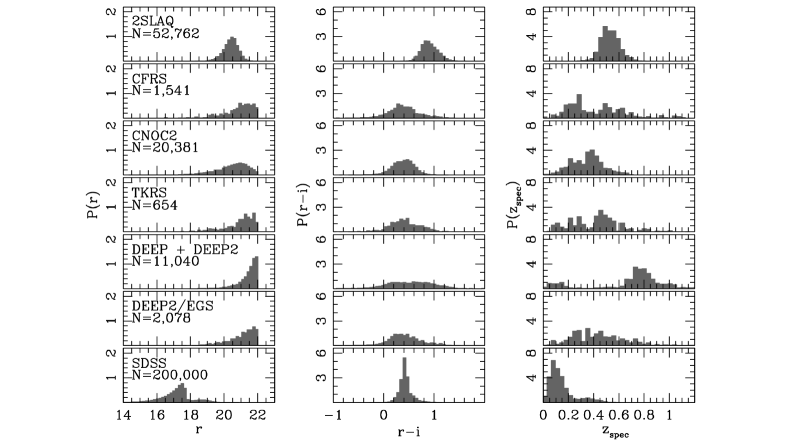
Therefore, we also test the weighting procedure using a combination of spectroscopic catalogs with SDSS DR6 photometry in $ugriz$ bands. The derived spectroscopic sample is similar to the one we used in constructing the DR6 galaxy photo-z catalog (Oyaizu et al., 2008), and we apply the same redshift quality and photometry cuts as were used there. Together these catalogs contain $288,456$ galaxies with $r<22$. We use $200,000$ galaxies from the SDSS DR6 main and LRG spectroscopic samples, $20,381$ from the Canadian Network for Observational Cosmology (CNOC) Field Galaxy Survey (CNOC2; Yee et al., 2000), $1,541$ from the Canada-France Redshift Survey (CFRS; Lilly et al., 1995), $11,040$ color-selected galaxies from the Deep Extragalactic Evolutionary Probe (DEEP; Davis et al., 2001) and the DEEP2 surveys (Weiner et al., 2005), $2,078$ galaxies from a roughly flux-limited sample from the Extended Groth Strip in DEEP2 (DEEP2/EGS; Davis et al., 2007), $654$ from the Team Keck Redshift Survey (TKRS; Wirth et al., 2004), and $52,762$ from the 2dF-SDSS LRG and QSO Survey (2SLAQ; Cannon et al., 2006) . The numbers of galaxies used from each catalog are smaller than those in Oyaizu et al. (2008), because we cut the samples at $r<22$, as opposed to the $r<23$ limit adopted in that work. Also, the numbers above include repeat objects due to repeat imaging in the SDSS BestRuns database, which was used to positionally match the galaxies.

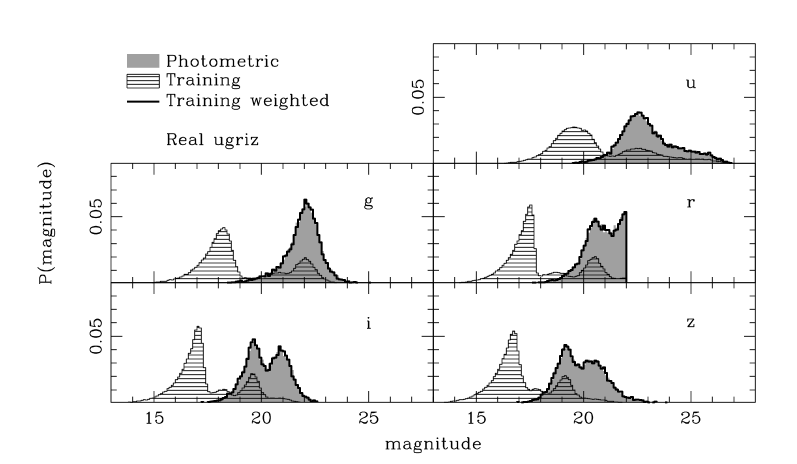
In Fig. 2, we show the distributions of $r$ magnitude, $r-i$ color, and spectroscopic redshift $z_{\rm spec}$ for each spectroscopic catalog. In combination, these data sets span a large range of magnitude, color, and redshift. We use these catalogs as a test case for our reconstruction methods of the redshift distribution below. In Cunha et al. (in preparation), we use simulations to investigate the effectiveness of the weighted $N(z)$ estimation on the SDSS DR6 Photoz2 sample described in Oyaizu et al. (2008).

3 The Weighting Method

The weighting method for reconstructing $N(z)$ for a photometric sample relies on the fact that a spectroscopic subsample of the galaxies with precisely measured redshifts is usually available. However, due to observational constraints, the spectroscopic subsample typically has different distributions of magnitudes, colors, and therefore redshift than the parent photometric sample, e.g., the spectroscopic sample may contain galaxies that are mostly much brighter than the flux limit of the photometric sample or the spectroscopic sample may be selected to lie within certain windows of color space. The weighting technique compensates for this mismatch by weighting galaxies in the spectroscopic sample so that the weighted sample has the same distribution of photometric observables (colors, magnitudes) as the parent photometric sample. The key assumption behind the method is that two samples with identical distributions of photometric observables will have identical distributions of redshift $N(z)$, so that the redshift distribution for the weighted spectroscopic sample serves as an estimate of the redshift distribution for the photometric sample. In § 6, we discuss the conditions that are required for this assumption to hold and the systematic errors that can arise for the $N(z)$ estimate if those conditions are not met.

In the remainder of this Section, we describe the construction of the weighting method.

3.1 Matching Distributions: Redshifts

We are interested in estimating $N(z)$ for a photometric set of interest. In practice, to estimate this distribution, we need to bin galaxies and compute the binned redshift distribution. Consider first binning the photometric and spectroscopic samples by non-overlapping redshift bins, denoted $i$ below. We define the normalized redshift distributions in the $i^{\rm th}$ redshift bin $[z^{i},z^{i}+\Delta z^{i}]$ in the photometric sample (superscript P) and in the spectroscopic training set (superscript T) as

$$P(z^{i})^{\rm P} \equiv \frac{1}{N_{\rm tot}^{\rm P}}\frac{N(z^{i})^{\rm P}}{\Delta z^{i}}=\frac{\rho(z^{i})^{\rm P}}{N_{\rm tot}^{\rm P}}\,,$$ (8)

$$P(z^{i})^{\rm T} \equiv \frac{1}{N_{\rm tot}^{\rm T}}\frac{N(z^{i})^{\rm T}}{\Delta z^{i}}=\frac{\rho(z^{i})^{\rm T}}{N_{\rm tot}^{\rm T}}\,,$$ (9)

where $N_{\rm tot}$ is the total number of galaxies in each catalog, $N(z^{i})$ is the number of galaxies in the $i^{\rm th}$ redshift bin, and we have defined the redshift density

$$\rho(z^{i})\equiv\frac{N(z^{i})}{\Delta z^{i}}\,.$$ (10)

In general, $P(z^{i})^{\rm T}\neq P(z^{i})^{\rm P}$. Using weights, we would like to transform $P(z^{i})^{\rm T}$ into a new distribution, $P(z^{i})^{\rm T}_{\rm wei}$, that provides an unbiased estimate of $P(z^{i})^{\rm P}$,

$$P(z^{i})^{\rm P}=\langle P(z^{i})^{T}_{\rm wei}\rangle\,.$$ (11)

To accomplish this, we weight objects in the spectroscopic training set according to their local density in the space of photometric observables.

To motivate the form of the weights, we first consider the idealized case of weighting directly in redshift. We seek a set of weights $W_{\alpha}$ for the spectroscopic training-set galaxies indexed by $\alpha$ such that the redshift distribution of the weighted training set is given by

$$P(z^{i})^{\rm T}_{\rm wei}\Delta z^{i}\equiv\frac{\sum_{\alpha=1}^{N(z^{i})^{\rm T}}{W_{\alpha}}}{\sum_{\alpha=1}^{N_{\rm tot}^{\rm T}}{W_{\alpha}}}\,,$$ (12)

where the sum in the numerator is over objects in the $i^{\rm th}$ redshift bin and that in the denominator is over all objects in the spectroscopic training set. The weights can be normalized by

$$\sum_{\alpha=1}^{N_{\rm tot}^{\rm T}}W_{\alpha}=1\,.$$ (13)

Clearly, Eq. (12) reduces to Eq. (9) if all objects have the same weight. We write the Eqs. above in terms of non-overlapping redshift bins because that is what we will show in our results after computing the galaxy weights $W_{\alpha}$. Consider now an alternate estimate of $N(z)$ with $overlapping$ bins centered at individual galaxies, indexed by $\beta$, with corresponding bin sizes $\Delta z_{\beta}$, possibly varying from galaxy to galaxy. All Eqs. (8-12) apply after substituting indices $i$ by $\beta$. For sufficiently narrow bins $\Delta z_{\beta}$, galaxies inside a given bin will be roughly indistinguishable and will have approximately equal weights, labeled $W_{\beta}$. In this case,

$$\sum_{\alpha=1}^{N(z_{\beta})^{\rm T}}{W_{\alpha}}\sim N(z_{\beta})^{\rm T}W_{\beta}\,.$$ (14)

Combining the results of Eqs. (8), (11)-(14) yields

$$\frac{1}{N_{\rm tot}^{\rm P}}\frac{N(z_{\beta})^{\rm P}}{\Delta z_{\beta}}=\frac{N(z_{\beta})^{\rm T}W_{\beta}}{\Delta z_{\beta}}\,,$$ (15)

from which it follows that the idealized weights are given by

$$W_{\beta}=\frac{1}{N_{\rm tot}^{\rm P}}\frac{\rho(z_{\beta})^{\rm P}}{\rho(z_{\beta})^{\rm T}}\,.$$ (16)

Of course, Eq. (16) is not useful in practice, since we do not know how to estimate the redshift density $\rho(z)^{P}$ for the photometric sample. In principle, one could do the matching in photo-z space, but photo-z estimates are subject to bias. Therefore we replace the redshift binning by an equivalent aperture in the photometric observables.

3.2 Matching Distributions: Observables

For concreteness we take the photometric observables to be the $N_{m}$ magnitudes of each galaxy, where $N_{m}$ is the number of filter passbands in the survey: the magnitude vector of the $\alpha^{\rm th}$ galaxy in a sample is ${\mn@boldsymbol{m}}_{\alpha}=m_{\alpha}^{a}$, with $a=1,...,N_{m}$. This choice of observables is not unique: we could instead use colors, morphological information, or any other photometric observable. A cell in magnitude space of radius $d_{m}$ defines an $N_{m}$-dimensional hypervolume, $V_{m}=d_{m}^{N_{m}}$. The magnitude density in multi-magnitude space at point ${\mn@boldsymbol{m}}$ within $V_{m}$ is defined as

$$\rho({\mn@boldsymbol{m}})\equiv\frac{N({\mn@boldsymbol{m}})}{V_{m}}\,,$$ (17)

where $N({\mn@boldsymbol{m}})$ is the number of objects in the corresponding magnitude region.

The redshift distribution of the photometric set can be rewritten as

$$P(z^{i})^{\rm P}=\frac{\rho(z^{i})^{\rm P}}{N_{\rm tot}^{\rm P}}=\int d{\mn@boldsymbol{m}}P(z^{i}|{\mn@boldsymbol{m}})^{\rm P}\frac{\rho({\mn@boldsymbol{m}})^{\rm P}}{N_{\rm tot}^{\rm P}}\,.$$ (18)

Similarly, the distribution of the weighted training is given by

$$P(z^{i})^{\rm T}_{\rm wei}=\rho(z^{i})^{T}W_{\alpha}=\int d{\mn@boldsymbol{m}}P(z^{i}|{\mn@boldsymbol{m}})^{\rm T}\rho({\mn@boldsymbol{m}})^{\rm T}W_{\alpha}\,.$$ (19)

Motivated by Eq. (16) and given our desire to set $P(z^{i})^{\rm T}_{\rm wei}=P(z^{i})^{\rm P}$, we redefine the galaxy weights – now as a function of magnitude densities – as

$$W_{\alpha}=\frac{1}{N_{\rm tot}^{\rm P}}\frac{\rho({\mn@boldsymbol{m}})^{\rm P}}{\rho({\mn@boldsymbol{m}})^{\rm T}}\,.$$ (20)

Therefore, the weighted training set distribution will provide an unbiased estimate of the true distribution in the photometric set if

$$\int d{\mn@boldsymbol{m}}P(z^{i}|{\mn@boldsymbol{m}})^{\rm P}\rho({\mn@boldsymbol{m}})^{\rm P} = \int d{\mn@boldsymbol{m}}P(z^{i}|{\mn@boldsymbol{m}})^{\rm T}\rho({\mn@boldsymbol{m}})^{\rm P}\,.$$ (21)

Notice that for a given magnitude ${\mn@boldsymbol{m}}$, there could be a broad range of possible redshifts $z$ due to degeneracies, and the weighting method would still work as long as Eq. (21) is satisfied. One obvious instance where this happens is if

$$P(z^{i}|{\mn@boldsymbol{m}})^{\rm P}=P(z^{i}|{\mn@boldsymbol{m}})^{\rm T},$$ (22)

i.e. if the training and photometric sets have the exact same degeneracies between redshift and magnitudes. A training set may violate this condition if it has selection effects that are very different from those of the photometric set. The selection effect can easily be accounted for if it happens in the space of observables. However, effects due to spectroscopic failure and large-scale structure (LSS) are more difficult to model and control.

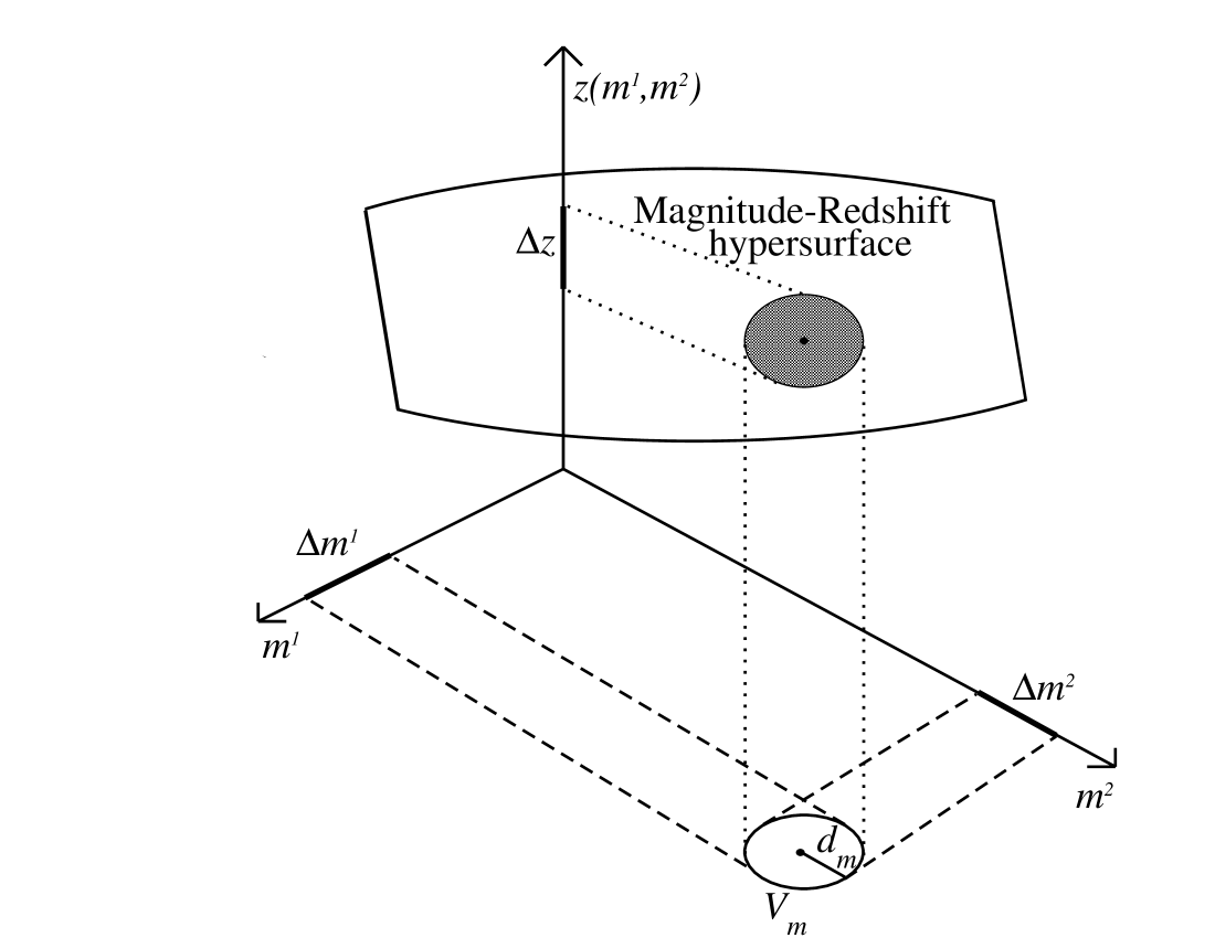
In the case where degeneracies are small, $P(z^{i}|{\mn@boldsymbol{m}})$ approaches a delta function $\delta(z^{i}|{\mn@boldsymbol{m}})$ and we have $\rho(z_{i})=\rho({\mn@boldsymbol{m}})$, i.e. the magnitude hypervolume $V_{m}$ specifies uniquely a corresponding cell in redshift $\Delta z$ as indicated in Fig. 3. The latter is typically the assumption of empirical photo-z methods; violation of this condition leads to photo-z biases and spurious peaks in the photo-z distribution. In contrast, the weighting method works more generally, since the only requirement is that the redshift distribution inside $V_{m}$ must be the same for training and photometric sets.

In order to calculate weights for training set galaxies using Eq. (20), we estimate the density $\rho({\mn@boldsymbol{m}})$ using the nearest-neighbor prescription described below.

3.3 Neighbors in Magnitude Space

Figure 3: Idealized magnitude-redshift hypersurface for $N_{m}=2$ magnitudes. Without degeneracies, the hypervolume in magnitude space surrounding a galaxy, $V_{m}\propto d_{m}^{N_{m}}$, corresponds to an approximate redshift interval $\Delta z$. Whereas empirical photo-z methods usually make this implicit assumption, the weighting method works under more general conditions.

A nearest-neighbor approach to calculating the density of galaxies in magnitude space is advantageous, because it enables control of statistical errors (shot noise) while also ensuring adequate “locality” of the cells in magnitude space. The distance $d_{\alpha\beta}$ in magnitude space between the $\alpha^{\rm th}$ and $\beta^{\rm th}$ galaxies in a (photometric or spectroscopic) sample is defined by

$$(d_{\alpha\beta})^{2}\equiv({\mn@boldsymbol{m}}_{\alpha}-{\mn@boldsymbol{m}}_{\beta})^{2}=\sum_{a=1}^{N_{m}}(m_{\beta}^{a}-m_{\alpha}^{a})^{2}\,.$$ (23)

We use this distance to find the set of nearest neighbors to the $\alpha^{\rm th}$ object, i.e., the set of galaxies with the smallest $d_{\alpha\beta}$. The density in magnitude space around this object, $\rho({\mn@boldsymbol{m}}_{\alpha})$, is then estimated as the ratio of the number of nearest neighbors $N_{\rm nei}$ to the magnitude hypervolume $V_{m}$ that they occupy, cf. Eq. (17). For fixed $N_{\rm nei}$, if we order the neighbors by their distance from the $\alpha^{\rm th}$ galaxy, then we can define the hypervolume by the distance from $\alpha$ to the $(N_{\rm nei})^{\rm th}$ (most distant) neighbor, indexed by $\gamma$, $V_{m}=(d_{\alpha\gamma})^{N_{m}}$.

Estimating the local density in the spectroscopic training set using a fixed (non-zero) value for $N({\mn@boldsymbol{m}}_{\alpha})^{\rm T}=N_{\rm nei}$ ensures that the density estimate is positive-definite and that the resulting weight is well defined. To estimate the corresponding density in the photometric sample, we simply count the number of galaxies in the photometric sample, $N({\mn@boldsymbol{m}}_{\alpha})^{\rm P}$, that occupy the same hypervolume $V_{m}$ around the point ${\mn@boldsymbol{m}}_{\alpha}$. Since the densities are estimated in the spectroscopic and photometric sets using the same hypervolume, the ratio of the densities is simply the ratio of the corresponding numbers of objects within the volume, and the weight for the $\alpha^{\rm th}$ training-set galaxy is therefore given by

$$W_{\alpha}=\frac{1}{N_{\rm tot}^{\rm P}}\frac{N({\mn@boldsymbol{m}}_{\alpha})^{\rm P}}{N({\mn@boldsymbol{m}}_{\alpha})^{\rm T}}\,.$$ (24)

The optimal choice of $N_{\rm nei}$ balances locality against statistical errors. By locality we mean that the distance to the $(N_{\rm nei})^{\rm th}$ nearest neighbor, $d_{\alpha\gamma}$, should ideally be smaller than the characteristic scale in magnitude space over which $\rho({\mn@boldsymbol{m}})$ varies; this argues for small hypervolumes, i.e., small values of $N_{\rm nei}$. On the other hand, if $N_{\rm nei}$ is chosen too small, the resulting estimate of the density, $\rho({\mn@boldsymbol{m}})=N_{\rm nei}/V_{m}$, will suffer from large shot-noise error. The resulting statistical error on the weight is

$$\frac{\delta W_{\alpha}}{W_{\alpha}}=\left[\frac{1}{N({\mn@boldsymbol{m}}_{\alpha})^{\rm P}}+\frac{1}{N({\mn@boldsymbol{m}}_{\alpha})^{\rm T}}\right]^{1/2}\,.$$ (25)

The optimal value of $N_{\rm nei}$ will depend on the characteristics of the photometric and spectroscopic samples at hand and should be determined using mock catalogs. For the DES and SDSS catalogs, we find in § 5 that the quality of the $N(z)$ reconstruction is relatively insensitive to the choice of $N_{\rm nei}$. The results we present there use the optimal values of $N_{\rm nei}$ determined by trial and error.

This implementation of the nearest-neighbor approach to estimating the magnitude-space densities and weights is not unique. For example, we could have instead used the same number of neighbors in both the spectroscopic and photometric samples, in which case the weights would be given by the ratio of corresponding hypervolumes,

$$W_{\alpha}=\frac{1}{N_{\rm tot}^{\rm P}}\left[\frac{(d_{\alpha\gamma})^{\rm T}}{(d_{\alpha\gamma^{\prime}})^{\rm P}}\right]^{N_{m}}\,,$$ (26)

where $\gamma^{\prime}$ indicates the $(N_{\rm nei})^{\rm th}$ nearest neighbor in the photometric sample. Our tests indicate that this produces similar results to the fixed hypervolume method, but that the latter is slightly more stable in sparsely occupied regions of the spectroscopic and photometric samples. In a region of magnitude space that is sparsely occupied in the photometric sample, using a fixed number of objects can result in a non-local estimate of the density. Fixing the hypervolume instead tends to avoid that problem. The results we present in § 5 use the fixed hypervolume, Eq. (24), to estimate the weights.

3.4 Weight Renormalization

If the spectroscopic training set has significantly different distributions of photometric observables than the photometric sample, then there may be galaxies in the training set that have very few or no neighbors in the photometric sample. Such galaxies will receive very small or zero weight and therefore make no contribution to the estimate of $N(z)^{\rm P}$. In this case, a recalculation of the weights may improve the accuracy of the redshift distribution reconstruction.

The idea is to perform a recalculation similar to a renormalization procedure. After an initial calculation of the weights, we remove objects from the training set that were assigned very small or zero weights. Using the objects that remain, the weights are recalculated, possibly using a smaller number of neighbors to achieve more locality of the new weights. This procedure can be iterated until some convergence of the weights is achieved.

As this renormalization procedure is iterated, the distribution in photometric observables of the remaining training set objects will approach that of the photometric sample, and the weights become more homogeneous.

We have found the renormalization to be useful if a large fraction of the training set objects have very small or zero weights. However, we do not expect to apply renormalization in practical situations, since the training set will typically be much smaller than the photometric set of interest. We suggest the use of simulations to study if the renormalization may help or not in each case. We present a case in which the renormalization significantly improves the weighting in § 5.

3.5 Summary of the Algorithm

To summarize, we outline the steps of the algorithm used to estimate the redshift distribution $N(z)$ of a photometric sample:

• For each galaxy $\alpha$ in the spectroscopic training set, find a fixed number $N({\mn@boldsymbol{m}}_{\alpha})^{\rm T}=N_{\rm nei}$ of its nearest neighbors in the training set according to the distance defined in Eq. (23) and compute the cell radius $d_{\alpha\gamma}$ as the distance to the $(N_{\rm nei})^{\rm th}$ nearest neighbor.

• Find the number $N({\mn@boldsymbol{m}}_{\alpha})^{\rm P}$ of objects in the photometric sample that fall within the same cell radius (volume).

• Compute the weight $W_{\alpha}$ according to Eq. (24).

• Repeat the weight calculation for each galaxy in the spectroscopic training set. Estimate the redshift distribution $P(z^{i})^{\rm P}$ by summing the weights for all training-set galaxies in the $i^{\rm th}$ redshift bin, cf. Eq. (12).

• If a large number of training-set galaxies have very low or zero weight, the renormalization procedure of § 3.4 can be implemented.

3.6 Weighting vs. Photo-z’s

It is worth contrasting the key assumption of the weighting method–that samples with identical distributions of photometric observables have identical distributions of redshift–with the stronger assumption implicit in training-set based photo-z estimates. Photo-z estimators assume that there is (and try to find) a functional correspondence between a set of photometric observables and redshift; degeneracies in that correspondence lead to photo-z biases. For the weighting method, all that is assumed is that values of the photometric observables uniquely determine the redshift probability distribution of galaxies with those observables, a distribution which may be multiply peaked, as long as these features appear in both the training and photometric sets. Moreover, the weights from a number of training-set galaxies are summed to estimate $N(z^{i})$ in a given redshift bin. If that number is reasonably large, this stacking will tend to cancel out possible statistical errors in individual galaxy weights. In Cunha et al. (in preparation), we show how the weighting procedure can be used to estimate a redshift distribution $p(z)$ for each galaxy in the photometric sample and thereby avoid the biases of photo-z estimates. Mandelbaum et al. (2007) show that using this weighted $p(z)$ in place of photo-z’s is very effective in reducing calibration biases in galaxy-galaxy weak lensing.

In § 5, we will present results for both the weighting method and photo-z estimates for comparison.

Figure 4: Distributions of magnitudes $grizY$ and colors $g-r$, $r-i$, $i-z$, $z-Y$, for the DES mock photometric catalog and for the first spectroscopic training set. Grey regions indicate the distributions in the photometric sample, horizontal hatched regions indicate those for the spectroscopic training set, and the solid black histograms are those for the weighted training set.

4 Measures of Reconstruction Quality

We measure the quality of the estimated redshift distribution reconstruction using two simple metrics. The first is the $\chi^{2}$ statistic (per degree of freedom and per galaxy), defined as

$$(\chi^{2})^{\rm X} = \frac{1}{N_{\rm bin}-1}\sum_{i=1}^{N_{\rm bin}}\frac{\left[P(z^{i})^{\rm X}-P(z^{i})^{\rm P}\right]^{2}}{P(z^{i})^{\rm P}}\,,$$ (27)

where $N_{\rm bin}$ is the number of redshift bins used, and $P(z^{i})^{\rm X}$ is equal to $P(z^{i})^{\rm T}_{\rm wei}$ if the weighting procedure is used or to $P(z_{\rm phot}^{i})^{\rm P}$ if the redshift distribution is instead estimated using photo-z’s. The usual definition of $\chi^{2}$ uses the numbers $N(z^{i})$ of objects in given bins instead of the normalized probability $P(z^{i})$; multiplying our $\chi^{2}$ by $\Delta zN_{\rm tot}$ gives the usual definition. We chose the above version so the resulting quantity is independent of the number of galaxies and the number of redshift bins. The definition allows us to more fairly compare reconstruction qualities across different data sets. Because the probabilities are normalized, the number of degrees of freedom is $N_{\rm bin}-1$.

The second metric we employ is the Kolmogorov-Smirnov (KS) statistic, defined as the maximum difference between the two cumulative redshift distributions being compared, for example, the cumulative distributions corresponding to $P(z^{i})^{\rm T}_{\rm wei}\Delta z$ and $P(z^{i})^{\rm P}\Delta z$. The KS statistic is more sensitive to the changes in the median of the two compared distributions whereas the $\chi^{2}$ tends to stress regions of the distribution that are least well sampled, i.e. regions where $P(z^{i})$ is small. In our implementation, we use binned cumulative distributions instead of unbinned cumulative distributions, and therefore our metric is not strictly the KS statistic.

It is important to stress that we do not associate any fundamental meaning to the absolute values of the metrics introduced above. They are used solely to compare the qualities of different reconstructions relative to each other.

For the DES mock catalogs, we use $N_{\rm bin}=50$ redshift bins covering the redshift interval $z=0-2$. For the real catalogs based on SDSS photometry, we use $N_{\rm bin}=30$ bins over $z=0-1.2$. In both sets of catalogs, the bins are equally sized in redshift.

5 Results

In this section, we test the methods of reconstruction of the redshift distribution on several simulated and real data sets.

5.1 DES mock catalog

Figure 5: Left panel: Photometric redshift $z_{\rm phot}$ vs. spectroscopic redshift $z_{\rm spec}$ for a random sampling of galaxies in the DES mock catalog. Photo-z’s were computed using the neural network algorithm described in Appendix A, using the first spectroscopic training set described in the text. The dashed and dotted curves are the contours containing $68\%$ and $95\%$ of the galaxies in narrow bins of $z_{\rm spec}$. Also indicated are the overall rms photo-z scatter $\sigma$ and $68\%$ confidence region $\sigma_{68}$ (see their definition in the text). Right panel: Redshift distributions. The shaded grey region shows the redshift distribution of the photometric sample that we are aiming to reconstruct. The horizontal hatched distribution shows the redshift distribution of the spectroscopic training set corresponding to the magnitude and color distributions shown in Fig. 4. The solid black histogram shows the reconstructed redshift distribution using the weighting method. The dotted lines show the neural network photo-z distribution of the photometric set, showing peaks due to photo-z biases. Also indicated are the $\chi^{2}$ and KS statistics for both the weighting method and the photo-z distribution.

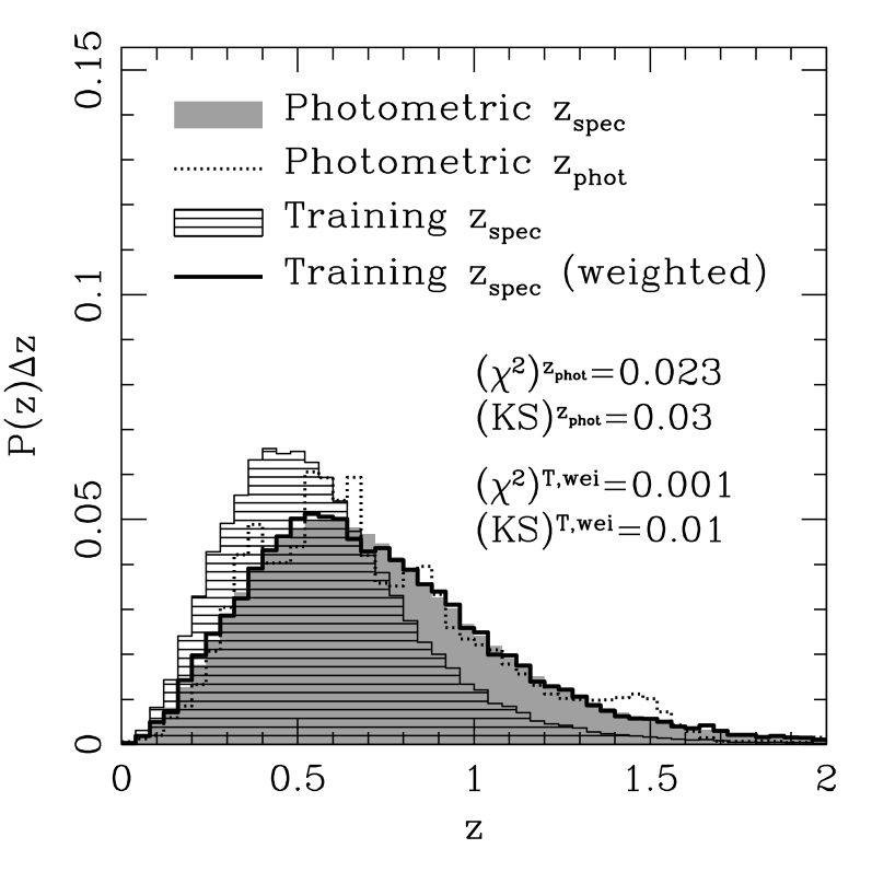
We first consider the DES mock photometric catalog of 500,000 galaxies described in § 2.1. We test the reconstruction using two spectroscopic training sets comprising $100,000$ galaxies each. Each of them have different distributions of magnitude, redshift, and galaxy type from the photometric sample.

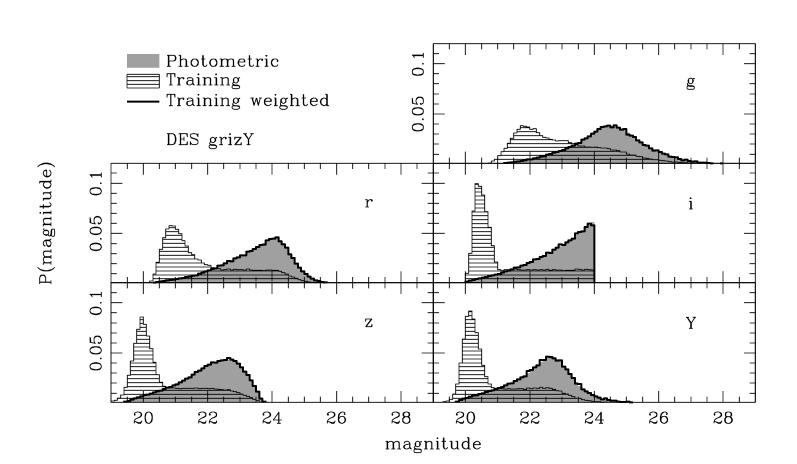
For the first training set, the magnitude and type distributions $P(i)$ and $P(t)$ differ from those of the photometric sample (recall the latter are given by Eq. (3) and Fig. 1), but the conditional redshift probability $P(z|i)$ is identical to that of the photometric sample, Eq. 4. In particular, the spectroscopic $i$-magnitude distribution, shown as the horizontal hatched region in Fig. 4, is skewed toward brighter magnitudes (and therefore lower redshift) than that of the photometric sample, with a peak at $i\simeq 20.5$, though it does include galaxies to the photometric limit, $i=24$. The spectroscopic type distribution $P(t)$ is chosen to be flat over the interval $t=-0.5$ to 3.5, in contrast to the bimodal photometric type distribution shown in Fig. 1. The spectroscopic type distribution may differ from that of the photometric sample due to, e.g., color selection in spectroscopic targeting or higher spectroscopic efficiency for certain galaxy types.

The weights were computed from Eq. 24, using the nearest neighbors in a fixed hypervolume in the space of all colors and $i$ magnitude. The hypervolume for each training set galaxy was defined by the $N_{\rm nei}=16$ nearest neighbors in the training set. Our tests indicated that this value of $N_{\rm nei}$ yields the lowest value for $\chi^{2}$ for the reconstruction in this case. However, as noted earlier, the results are not sensitive to this choice. Increasing $N_{\rm nei}$ to 64 causes a negligible change in $\chi^{2}$, while decreasing it to 4 causes an increase of less than 20% in $\chi^{2}$.

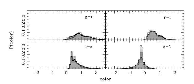
Figs. 4 and 5 display the reconstruction results for this case using the weighting method. Fig. 4 shows the distributions of magnitudes and colors for the photometric sample (solid grey), the spectroscopic training sample (horizontal hatched), and the weighted training set (black line). The coincidence of the grey and black regions demonstrates that the weighted training set distributions in magnitudes and colors are excellent matches to those of the photometric sample. The right panel of Fig. 5 shows that the weighted training-set redshift distribution also provides a precise estimate of the redshift distribution of the photometric sample. The measures of reconstruction quality for this match are $(\chi^{2})^{\rm T,wei}=0.001$ and (KS)${}^{\rm T,wei}=0.01$.

Figure 6: As Fig. 5, but now using the second spectroscopic training set described in the text. In this case, the training set is even less representative of the photometric sample than in the previous example, but the weighting procedure still accurately reconstructs the redshift distribution of the photometric sample.

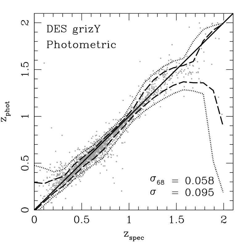
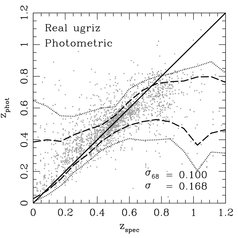
For comparison, we also carry out the $N(z)$ reconstruction using photometric redshift estimates. The left panel of Fig. 5 shows the photo-z scatter for the neural network photo-z estimator described in Appendix A. Here the spectroscopic set has been split into 2 samples (the training and validation sets) of equal sizes that were used to train and validate the network, which was finally applied to compute photo-z’s for the photometric sample. To test the overall quality of the photo-z estimates we use two photo-z performance metrics, whose values are also displayed in Fig. 5. The first metric is the photo-z rms scatter, $\sigma$, averaged over all $N$ objects in the photometric set, defined by

$$\sigma^{2} = \frac{1}{N}\sum_{i=1}^{N}\left(z_{\rm phot}^{i}-z_{\rm spec}^{i}\right)^{2}~{},$$ (28)

whereas, the second performance metric, denoted by $\sigma_{68}$, is the range containing $68\%$ of the photometric set objects in the distribution of $\delta z=z_{\rm phot}-z_{\rm spec}$. We also define similarly $\sigma_{68}$ and $\sigma_{95}$ in bins of $z_{\rm spec}$, and the dashed and dotted lines in the left panel of Fig. 5 show these regions respectively.

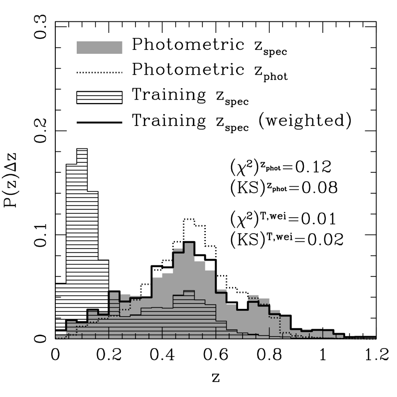
The right panel of Fig. 5 shows the resulting $N(z_{\rm phot})$ distribution for the photometric sample (dotted line). Due to degeneracies in the relation between magnitudes and redshift, the photo-z estimate is biased at low and high redshifts. In particular, the photo-z solution produces an excess of galaxies at $z_{\rm phot}\approx 0.4$, 0.6, and $1.4$, which translates into the spurious peaks at these redshifts in the right panel of Fig. 5. The corresponding measures of reconstruction quality are $(\chi^{2})^{z_{\rm phot}}=0.023$ and (KS)${}^{z_{\rm phot}}=0.03$, significantly worse than those for the weighting method. Deconvolution of the $N(z_{\rm phot})$ distribution can improve this match (Padmanabhan et al., 2005); we will explore that elsewhere (Cunha et al., in preparation).

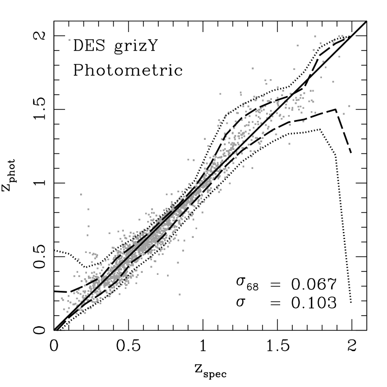
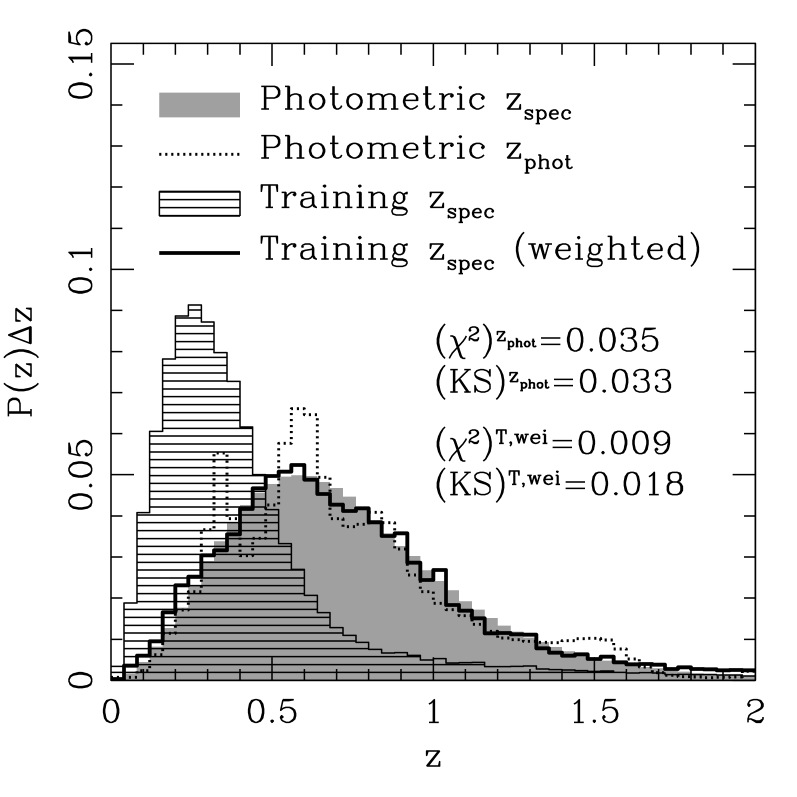
For the second training set example, we make the spectroscopic sample even less representative of the photometric sample. We keep the spectroscopic $i$-magnitude and type distributions of the previous example, but we alter the conditional redshift probability $P(z|i)$ of the training set so that it is more concentrated toward lower redshift while still covering the redshift range $z\in[0,2]$. Specifically, we change the parameter values that determine $z_{d}$ and $\sigma_{d}$ in Eqs. (5) and (6) to $(b_{1},b_{2},b_{3})=(-0.5,0.6,-0.5)$ and $(c_{1},c_{2},c_{3})=(0.38,0.02,3.5)$. By decreasing the values of $b_{i}$ relative to those of the photometric sample, we shift the distribution toward lower redshift, while increasing $c_{2}$ and $c_{3}$ increases the spread of the distribution in redshift so that the full range to $z=2$ is still covered. This example could correspond, for instance, to a training set that is obtained by combining different spectroscopic surveys with different selection functions. Notice that changing only $P(z|i)$ means that we are changing only one dimension of the probability $P(z|{\mn@boldsymbol{m}})$ which lives in a 5-dimensional space of magnitudes. If there are no further selection effects, we still expect the weighting method to work reasonably well, though obviously not as accurately as in the first case of Fig. (5).

In this case, we find that $N_{\rm nei}=4$ neighbors is nearly optimal: training sets that are less representative require fewer neighbors to provide the best match, since locality in magnitude/color space becomes more important. The redshift distribution of the photometric sample estimated from the weighted training set is shown in the right panel of Fig. 6. (As in the previous example, the weighted reconstructions of the magnitude and color distributions are nearly perfect, as in Fig. 4, so we do not show them.) Even though the training-set redshift distribution is now considerably different from that of the photometric sample, peaking at $z\sim 0.25$ as opposed to $z\sim 0.6$, the weighting method still does a very good job of estimation, with $(\chi^{2})^{\rm T,wei}=0.009$ and (KS)${}^{\rm T,wei}=0.018$.

The left panel of Fig. 6 shows the scatter plot for the neural network photo-z estimates for this training set; the photo-z scatter is larger than in the previous example, as expected since the training set is less representative of the photometric sample. As the right panel of Fig. 6 also shows, the photo-z distribution has spurious peaks at the same redshifts as before, but they are now more pronounced. The photo-z distribution has $(\chi^{2})^{z_{\rm phot}}=0.035$ and (KS)${}^{z_{\rm phot}}=0.033$, significantly worse than for the weighting method.

5.2 SDSS Data Catalogs

Figure 7: Distributions of magnitudes ($ugriz$) and colors ($u-g$, $g-r$, $r-i$, $i-z$) for samples drawn from SDSS DR6 photometry, for the first example in the text in § 5.2. Grey regions denote the distributions in the photometric sample, horizontal hatched regions are for the spectroscopic training set, and the black histograms show the reconstructed distributions for the photometric sample using the weighted training set.

Figure 8: Left panel: Scatter of neural network photo-z estimates using the same training set and photometric sample as in Fig. 7. Right panel: Redshift distributions for the photometric sample, spectroscopic training set, weighted training set, and photo-z’s.

Here we consider two examples of the reconstruction of the redshift distribution for photometric samples drawn from the SDSS, using the spectroscopic samples described in § 2.2 and shown in Fig. 2.

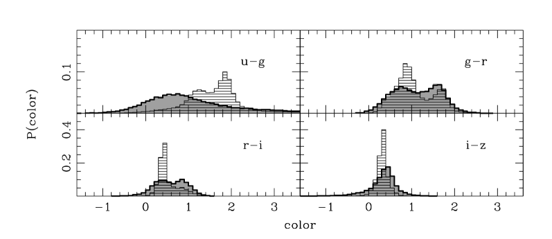
For the first case, we created a spectroscopic training set comprising $200,000$ galaxies from the SDSS spectroscopic survey, $15,000$ galaxies from CNOC2, $6,000$ from the DEEP+DEEP2 sample, and $47,000$ from 2SLAQ, for a total of $268,000$ galaxies. For all these sets, the galaxies were randomly selected from the parent spectroscopic sample. The photometric sample comprises the remaining galaxies with spectroscopic redshifts, namely $5,381$ galaxies from CNOC2, $1,541$ from CFRS, $5,040$ from DEEP+DEEP2, $2,078$ from DEEP2/EGS, $654$ from TKRS, and $5,762$ from 2SLAQ, for a total of $20,456$ galaxies.

For this example, we calculated weights for the training-set galaxies using a hypervolume in color/$r$-magnitude space with $N_{\rm nei}=32$ neighbors. Fig. 7 shows the magnitude and color distributions for the photometric sample, the spectroscopic training set, and the weighted training set. The weighting procedure provides an excellent match to the distributions for the photometric sample. This is not a difficult test for the method since, with the exception of the SDSS spectroscopic sample, the distributions for the training and photometric samples are rather similar and by construction Eq. (22) is satisfied. The right panel of Fig. 8 shows the corresponding redshift distributions for these training and photometric samples. The weighted training set provides a good estimate of $N(z)$ for the photometric sample, with $(\chi^{2})^{\rm T,wei}=0.01$ and (KS)${}^{\rm T,wei}=0.02$. The left panel of Fig. 8 shows the photo-z scatter for the neural network photo-z estimator trained on the same spectroscopic sample and applied to the photometric sample. The biases at low and high redshift are evident. The photo-z distribution shown in the right panel of Fig. 8 provides a less accurate representation of the true redshift distribution of the photometric sample than the weighting procedure–features in the true redshift distribution are smoothed out, and the distribution is systematically underestimated at high redshift; the corresponding $(\chi^{2})^{z_{\rm phot}}=0.12$ and (KS)${}^{z_{\rm phot}}=0.08$ are again considerably worse than for the weighting procedure.

For the second case, the training set and the photometric sample come from different spectroscopic surveys. Here, the training set comprises the galaxies from all the spectroscopic surveys with the exception of the DEEP2/EGS catalog, and the latter is taken to be the photometric sample. The training set contains $286,378$ galaxies, and the photometric sample $2078$. Since DEEP2/EGS is – apart from the match to SDSS photometry – roughly flux limited, this provides a more realistic case, except for the fact that the photometric sample in practice would typically be much larger.

In this case, since the training set is much larger than the photometric sample, the best results are achieved if the weights are renormalized according to the procedure described in § 3.4. However let us first consider what happens if we do not apply renormalization and compute the weights only once as in all previous cases.

Matching both colors and $r$-magnitude is better achieved with high number of neighbors. The maximum number we chose was $N_{\rm nei}=4096$, in which case we obtain $(\chi^{2})^{\rm T,wei}=0.29$. On the other hand, if we only perform the match in color space, the best results happen with $N_{\rm nei}=1$ and also produce $(\chi^{2})^{\rm T,wei}=0.29$. In the first case, we find that the redshift distribution is well reconstructed at low redshifts, but overestimated at higher redshifts, whereas the opposite happens in the latter case of matching only the color distributions. These features suggest that we employ the following renormalization procedure described below.

Figure 9: Left panel: Neural network photo-z scatter for the second case described in § 5.2, which uses DEEP2/EGS as the photometric sample and all other spectroscopic catalogs for the training set. Right panel: Redshift distributions for the photometric sample, training set, weighted training set, and photo-z.

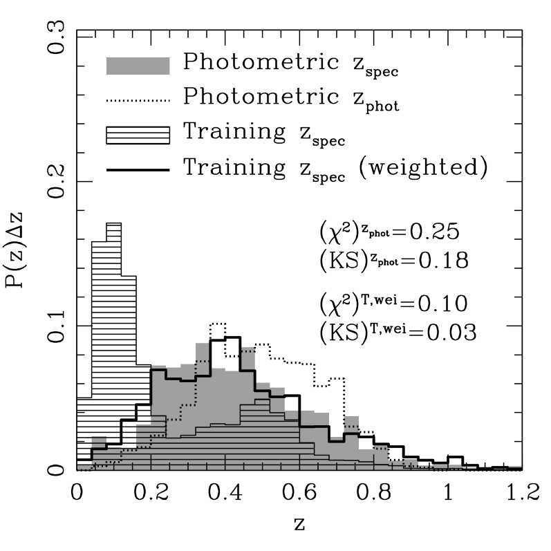
We first calculate the weights by matching the distributions of colors and magnitudes using $N_{\rm nei}=4096$ neighbors in the training set. After this first calculation, more than half of the training set galaxies have zero weights and are removed from the catalog. We then iterate the weight calculation by matching only the color distributions. In each iteration, we remove objects with zero weight and reduce $N_{\rm nei}$ by a factor of 2 until $N_{\rm nei}=1$. Only $7,968$ of the original training-set galaxies have positive weight in the final iteration. The right panel of Fig. 9 shows the resulting redshift distributions for this case; for the renormalized weighting procedure, the reconstruction has $(\chi^{2})^{\rm T,wei}=0.10$, while the corresponding photo-z distribution has $(\chi^{2})^{\rm z_{\rm phot}}=0.25$; likewise (KS)${}^{\rm T,wei}=0.03$ whereas (KS)${}^{z_{\rm phot}}=0.18$. It is clear that the weighting method provides a better estimate of $N(z)$.

Given the small size of the photometric sample, there is considerable shot noise in its redshift distribution. In addition, the small angular-area of the survey introduces significant LSS effects in the redshift distribution (see e.g. Mandelbaum et al., 2007). The weighted reconstruction works well in spite of these complications.

Because we need to go down to $N_{\rm nei}=1$, imposed by the locality requirement, Poisson errors of individual galaxy weights are relatively large. However, given the large number of galaxies in each redshift bin, these errors cancel out and the overall reconstruction is improved.

This case illustrates that this method has the potential to provide very accurate estimations of the redshift distributions of flux limited samples in future galaxy surveys, even when they are subject to LSS effects.

6 Discussion

We have presented a new technique to estimate the underlying redshift distribution of photometric galaxy samples. The method relies on a spectroscopic training set and re-weighting of the training-set galaxies to match the distribution of photometric observables of the photometric sample. The weights are estimated using a flexible nearest-neighbor approach in color-magnitude space and the redshift distribution is estimated by summing the galaxy weights in redshift bins. Tests on mock catalogs and on existing data sets show that this procedure yields an accurate estimate of the redshift distribution and that it performs significantly better than simply binning the photo-z estimates of individual galaxies in the photometric sample. The weighting method also appears to be robust, in the sense that the spectroscopic sample can have very different distributions of photometric observables and redshift from the photometric sample. The main requirement is that the training set should span the range of photometric observables found in the photometric sample.

The key assumption underlying the technique is that two samples (e.g., the spectroscopic and photometric) with the same distribution of photometric observables will have very similar redshift distributions. This assumption holds if the selection criteria used to define the two samples differ only in the space of photometric observables. Several effects can cause this condition to be violated: statistical errors, LSS and spectroscopic failures.

Statistical errors are the simplest to quantify and are significant in regions of magnitude space where the training set is sparse, typically at fainter magnitudes. LSS can be significant if certain regions of the space of photometric observables are only represented in the training set by a survey that covers small solid angle, in which one or a few large structures dominate. We showed that, even in such cases, the weighting method works quite well (§ 5.2).

Spectroscopic failures (i.e., targeted objects for which a redshift could not be obtained) in the training set can have a similar effect if the failures happen systematically, for instance in a particular galaxy spectral type. If the effects of spectroscopic failures are prevalent in regions of magnitude space where the redshift distribution is broad or multiply peaked, they can potentially cause systematic errors in the recovery of the redshift distribution. However we also showed that the weighting method performs well even when we take an arbitrary type distribution in the training set (§ 5.1).

The weighting method requires a training set with a size (density) such that the inter-(training-set)-galaxy separation in the space of photometric observables is comparable to the characteristic (curvature) scale of the redshift/photometric-observables manifold or the scale defined by the typical photometric errors - whichever is smaller. That condition ensures that on average at least one neighbor to the galaxy is meaningful; in practice it would be safer to have the density a few times larger than this minimum density. The use of mock catalogs can shed light on the optimal parameters to employ on the weighting method, such as the number of neighbors $N_{\rm nei}$ (possibly varying according to the local density), the minimum training set size, the need or not for renormalization, etc. Since these simulations are necessary for other typical calibration reasons, their need does not put any strong restrictions to the application of the weighting method. For instance, simulations and calibration samples are necessary to calibrate the photo-z errors.

This weighting technique has been used to estimate the redshift distribution of the SDSS DR6 photometric sample (Oyaizu et al., 2008) and to help assess the quality of the photo-z’s computed for that sample. It has also been used in conjunction with photo-z’s in the measurement of the SDSS cluster-mass cross-correlation function via weak lensing (Sheldon et al., 2007a), allowing for the inversion of cluster mass profiles (Johnston et al., 2007) and estimation of cluster mass-richness relations (Johnston et al., 2007) and mass-to-light ratios (Sheldon et al., 2007b). Finally, this weighting scheme has recently been employed in the study of galaxy-galaxy weak lensing calibration bias (Mandelbaum et al., 2007), where it was shown to yield much smaller biases than those arising from photo-z estimates. For future photometric surveys, the weighting method can complement and provide cross-checks on photo-z estimates and help control photo-z errors.

Appendix A Artificial Neural Network Photo-z’s

For comparison with the weighting method, we use an Artificial Neural Network (ANN) method to estimate photometric redshifts (Collister & Lahav, 2004; Oyaizu et al., 2008) We use a particular type of ANN called a Feed Forward Multilayer Perceptron (FFMP), which consists of several nodes arranged in layers through which signals propagate sequentially. The first layer, called the input layer, receives the input photometric observables (magnitudes, colors, etc.). The next layers, denoted hidden layers, propagate signals until the output layer, whose outputs are the desired quantities, in this case the photo-z estimate. Following the notation of Collister & Lahav (2004), we denote a network with $k$ layers and $N_{i}$ nodes in the $i^{\rm th}$ layer as $N_{1}:N_{2}:...:N_{k}$.

A given node can be specified by the layer it belongs to and the position it occupies in the layer. Consider a node in layer $i$ and position $\alpha$ with $\alpha=1,2,...,N_{i}$. This node, denoted $P_{i\alpha}$, receives a total input $I_{i\alpha}$ and fires an output $O_{i\alpha}$ given by

$$O_{i\alpha}=F(I_{i\alpha})\,,$$ (29)

where $F(x)$ is the activation function. The photometric observables are the inputs $I_{1\alpha}$ to the first layer nodes, which produce outputs $O_{1\alpha}$. The outputs $O_{i\alpha}$ in layer $i$ are propagated to nodes in the next layer $(i+1)$, denoted $P_{(i+1)\beta}$, with $\beta=1,2,..N_{i+1}$. The total input $I_{(i+1)\beta}$ is a weighted sum of the outputs $O_{i\alpha}$

$$I_{(i+1)\beta}=\sum_{\alpha=1}^{N_{i}}w_{i\alpha\beta}O_{i\alpha},$$ (30)

where $w_{i\alpha\beta}$ is the weight that connects nodes $P_{i\alpha}$ and $P_{(i+1)\beta}$. Iterating the process in layer $i+1$, signals propagate from hidden layer to hidden layer until the output layer. There are various choices for the activation function $F(x)$ such as: a sigmoid, a hyperbolic tangent, a step function, a linear function, etc. This choice typically has no important effect on the final photo-z’s, and different activation functions can be used in different layers. Training the network consists in finding weights $w_{i\alpha\beta}$ that best reproduce the true redshifts $z_{\rm spec}$ in a spectroscopic validation set.

In our implementation, we use a network configuration $N_{m}:15:15:15:1$, which receives $N_{m}$ magnitudes and outputs a photo-z. We use hyperbolic tangent activation functions in the hidden layers and a linear activation function for the output layer.

References

- Banerji et al. (2007) Banerji M., Abdalla F. B., Lahav O., Lin H., 2007, ArXiv e-prints, 711
- Bruzual & Charlot (1993) Bruzual A. G., Charlot S., 1993, Astrophys. J., 405, 538
- Cannon et al. (2006) Cannon R., et al., 2006, Mon. Not. R. Astron. Soc., 372, 425
- Capak et al. (2004) Capak P., et al., 2004, Astron. J., 127, 180
- Coleman et al. (1980) Coleman G. D., Wu C. C., Weedman D. W., 1980, Astrophys. J. Supp., 43, 393
- Collister & Lahav (2004) Collister A. A., Lahav O., 2004, Pub. Astron. Soc. Pacific, 116, 345
- Cowie et al. (2004) Cowie L. L., Barger A. J., Hu E. M., Capak P., Songaila A., 2004, Astron. J., 127, 3137
- Davis et al. (2007) Davis M., et al., 2007, Astrophys. J. Lett., 660, L1
- Davis et al. (2001) Davis M., Newman J. A., Faber S. M., Phillips A. C., 2001, in Cristiani S., Renzini A., Williams R. E., eds, Deep Fields The DEEP2 Redshift Survey. pp 241–+
- Huterer et al. (2004) Huterer D., Kim A., Krauss L. M., Broderick T., 2004, Astrophys. J., 615, 595
- Huterer et al. (2006) Huterer D., Takada M., Bernstein G., Jain B., 2006, MNRAS, 366, 101
- Jain et al. (2007) Jain B., Connolly A., Takada M., 2007, Journal of Cosmology and Astro-Particle Physics, 3, 13
- Johnston et al. (2007) Johnston D. E., et al., 2007, ArXiv e-prints, 709
- Lilly et al. (1995) Lilly S. J., Le Fevre O., Crampton D., Hammer F., Tresse L., 1995, Astrophys. J., 455, 50
- Lima & Hu (2007) Lima M., Hu W., 2007, Phys. Rev. D, 76, 123013
- Lin et al. (1999) Lin H., et al., 1999, Astrophys. J., 518, 533
- Ma et al. (2006) Ma Z., Hu W., Huterer D., 2006, Astrophys. J., 636, 21
- Mandelbaum et al. (2007) Mandelbaum R., et al., 2007, ArXiv e-prints, 709
- Oyaizu et al. (2008) Oyaizu H., Lima M., Cunha C. E., Lin H., Frieman J., Sheldon E. S., 2008, ArXiv e-prints, 708
- Padmanabhan et al. (2005) Padmanabhan N., et al., 2005, Mon. Not. R. Astron. Soc., 359, 237
- Poli et al. (2003) Poli F., et al., 2003, Astrophys. J. Lett., 593, L1
- Sheldon et al. (2004) Sheldon E. S., et al., 2004, Astron. J., 127, 2544
- Sheldon et al. (2007a) Sheldon E. S., et al., 2007a, ArXiv e-prints, 709
- Sheldon et al. (2007b) Sheldon E. S., et al., 2007b, ArXiv e-prints, 709
- Sheth (2007) Sheth R. K., 2007, Mon. Not. R. Astron. Soc., 378, 709
- Weiner et al. (2005) Weiner B. J., et al., 2005, Astrophys. J., 620, 595
- Wirth et al. (2004) Wirth G. D., et al., 2004, Astron. J., 127, 3121
- Yee et al. (2000) Yee H. K. C., et al., 2000, Astrophys. J. Supp., 129, 475
- Zhan (2006) Zhan H., 2006, JCAP, 0608, 008
- Zhan & Knox (2006) Zhan H., Knox L., 2006, Astrophys. J., 644, 663