Magnetic flux noise in the three Josephson junctions superconducting ring

Abstract

We analyze the influence of noise on magnetic properties of a superconducting loop which contains three Josephson junctions. This circuit is a classical analog of a persistent current (flux) qubit. A loop supercurrent induced by external magnetic field at the presence of thermal fluctuations is calculated. In order to get connection with experiment we calculate the impedance of the low-frequency tank circuit which is inductively coupled with a loop of interest. We compare obtained results with the results in quantum mode - when the three junction loop exhibits quantum tunneling of the magnetic flux. We demonstrate that the tank-loop impedance in the classical and quantum modes have different temperature dependence and can be easily distinguished experimentally.

PACS: 85.25.Am Superconducting device characterization, design, and modeling;
85.25.Hv Superconducting logic elements and memory devices; microelectronic circuits.

Keywords: Josephson junction; SQUID; Flux qubit; Thermal fluctuations

1 Introduction

Magnetic flux quantization in superconductors is used, in particular, for realization of very sensitive magnetometers. One of them is so-called radio-frequency (rf) SQUID [1]. The sensor of rf SQUIDs is a single junction interferometer - a Josephson junction which is incorporated in a superconducting ring with a sufficiently small inductance $L$. When an external flux $\Phi_{e}$ is applied to an interferometer loop, the circulating supercurrent $I$ is induced and a flux $\Phi_{i}$ is admitted into the ring:

$$\Phi_{i}=\Phi_{e}-IL.$$ (1)

The phase difference $\varphi$ across a Josephson junction equals to a normalized magnetic flux in the interferometer loop:

$$\varphi=2\pi\frac{\Phi_{i}}{\Phi_{0}}+2\pi n.$$ (2)

where $\Phi_{0}$ is the flux quantum, and $n$ is an integer. Since the Josephson current is related to the phase difference $\varphi$:

$$I=I_{c}sin\varphi,$$ (3)

where $I_{c}$ is the critical current, Eq. 1 can be rewritten:

$$\varphi=\varphi_{e}-\beta sin\varphi$$ (4)

where $\varphi_{e}=2\pi{\Phi_{e}}/{\Phi_{0}}$ is the normalized external flux and the constant

$$\beta=2\pi LI_{c}/\Phi_{0}$$ (5)

is the normalized inductance of the interferometer.

From Eq. 4 it is clearly seen that the magnetic properties of a single junction interferometer are defined by parameter $\beta$. If $\beta<1$ the $\varphi_{e}(\varphi)$ dependence is unique (see Fig. 1) and corresponding mode of SQUID operation is so-called nonhysteretic. If $\beta>1$ the $\varphi_{e}(\varphi)$ dependence is multivalued (see Fig. 1) and corresponding mode of SQUID operation is hysteretic.

A rf SQUID basically consists of a sensor (usually a single junction interferometer) inductively coupled to a radio-frequency-biased tank circuit. The flux $\varphi_{e}$ applied to the sensor changes the effective inductance (or/and the effective resistance) of the tank-sensor arrangement. Thus, a flux change can be detected as changes in phase (or/and amplitude) of the voltage across the tank circuit.

The classical mode for the single junction interferometer as well as for corresponding rf SQUID in the presence of fluctuations have been investigated in detail theoretically as well as experimentally [2-7]. On the other hand the quantum mode for this device is difficult to realize. Since an interferometer should be hysteretic, it requires the finite $LI_{c}$ product, and therefore, the finite coupling with environment. In order to avoid this problem, a substitution of the geometrical inductance to the Josephson one has been proposed. Indeed, if the number of Josephson junctions in the loop $m>2$ and for suitable junctions parameters, a double degenerated state exists at any geometrical inductance $L$. One of the simplest realizations here is a three- junction interferometer, which is called also a persistent current (or flux) qubit [8]. Such qubit was fabricated by several teams and quantum regime was convincingly demonstrated.

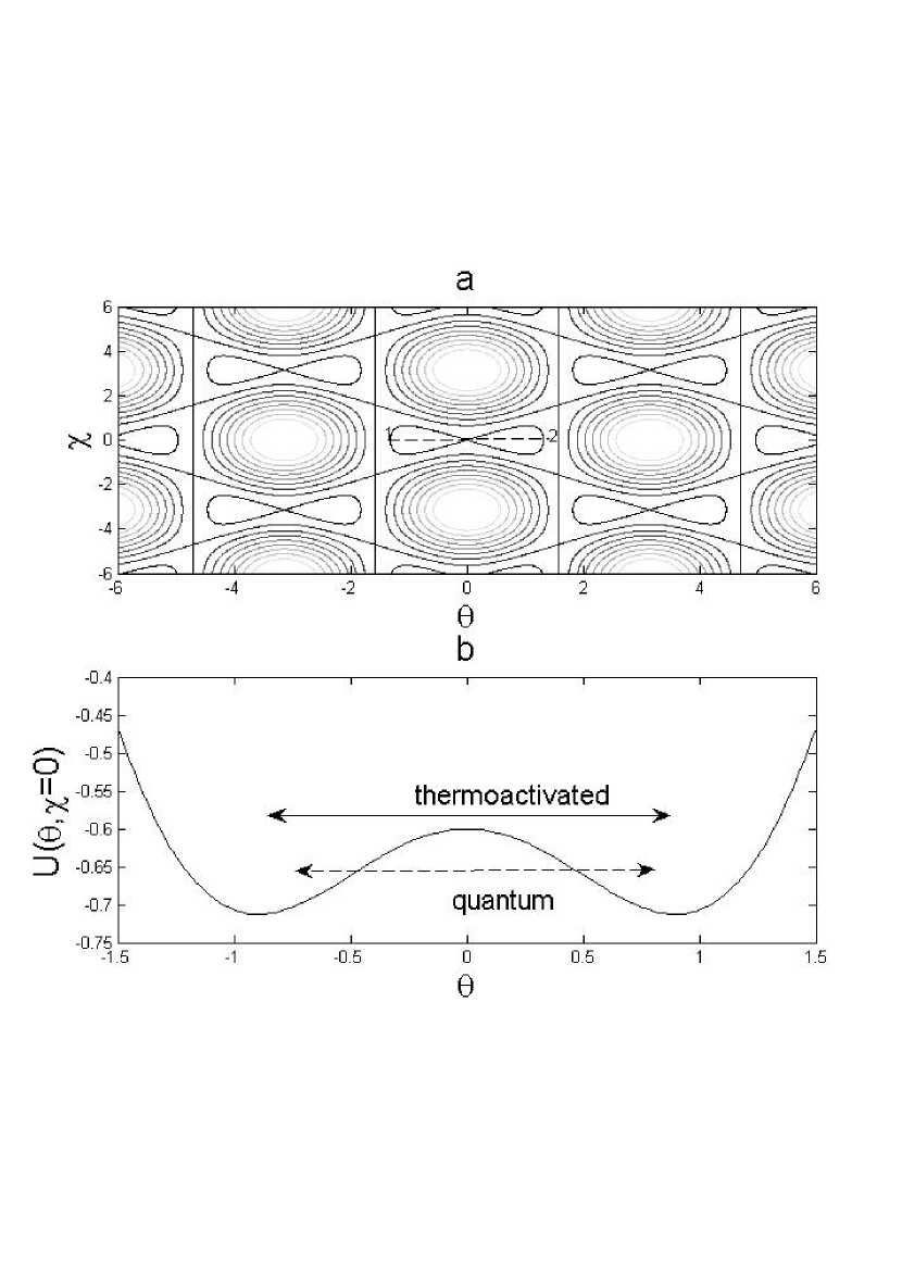
If external magnetic flux is

$$\varphi=\pi+2\pi n.$$ (6)

the hysteretic interferometer exhibits double-degenerated energy states, see Fig. 3. These states correspond to the different directions of the interferometer current. If temperature is low enough and for suitable parameters of Josephson junctions the magnetic flux can tunnel between the two potential minima. Below we will call the systems under consideration quantum if in their dynamics there is quantum tunneling. If, for some reasons, the quantum tunneling is suppressed, we will call these systems classical ones.

It is clear that the presence of the quantum tunneling ensures the absence of the hysteresis at the $\varphi_{e}(\varphi)$ dependence. On the other hand jumps between two energy minima can be originated by the fluctuations and the hysteresis will be washed out. Therefore for both cases considered above the mode of the rf SQUID operation will be nonhysteretic. It arises a natural question: by analyzing a SQUID output signal is it possible to distinguish between quantum mode (interferometer with ”quantum leak”) and classical mode (interferometer in presence of the fluctuations)? We address this paper to that question.

2 Classical mode of a flux qubit in the presence of fluctuations

The studied system presents the superconducting circuit (ring) with three Josephson junctions, see Fig. 2. We consider the case of small self inductance of the ring $L\rightarrow 0$, therefore $\Phi_{e}=\Phi_{i}$. The phases across each junction in the qubit loop $\varphi_{i}$ satisfy to

$$\varphi_{1}+\varphi_{2}+\varphi_{3}=\varphi_{e}.$$

In the frame of RSJ model for Josephson junctions the current through each junction is:

$$I=\frac{\hbar C_{i}}{2e}\frac{d^{2}}{dt^{2}}\varphi_{i}+\frac{\hbar}{2eR_{i}}\frac{d}{dt}\varphi_{i}+I_{ci}\sin\varphi_{i}+\delta I_{i}(t),i=1,2,3$$ (7)

where $\hbar$ is the Plank constant, $e$ is the electron charge, $C_{i}$ and $R_{i}$ are the junctions’ capacitances and resistances respectively. We restrict ourself to a practical case, when two junctions in the loop are identical: $C_{1}=C_{2}=C,I_{c1}=I_{c2}=I_{c},R_{1}=R_{2}=R$ and the third junction has slightly smaller critical current (with the same critical current density) $I_{c3}=\alpha I_{c},0.5<\alpha<1$ and therefore $C_{3}=\alpha C,R_{3}=R/\alpha$. The presence of the ’white noise’ is given by the fluctuation currents $\delta I_{i}(t)$ with correlator $<\delta I_{i}(t)\delta I_{i}(t^{{}^{\prime}})>=2kT/R_{i}\delta(t-t^{{}^{\prime}})$ and mean value $<\delta I_{i}(t)>=0$.

In dimensionless units:

$$\omega_{R}=2eRI_{c}/\hbar,\omega_{R}t=\tau\\$$ (8)

and for negligible capacitance, Eq. 7 can be rewritten:

$$I/I_{c}=d\varphi_{1,2}/d\tau+\sin\varphi_{1,2}+\delta\varphi_{1,2}=\alpha d\varphi_{3}/d\tau+\alpha\sin\varphi_{3}+\delta\varphi_{3}(\tau).$$ (9)

The correlators of $\delta\varphi_{i}$ are:

$$<\delta\varphi_{i}(\tau)\delta\varphi_{i}(\tau^{{}^{\prime}})>=2D\delta_{i}(\tau-\tau^{{}^{\prime}}),$$ (10)

where $D=kT/E_{J}$, $E_{J}=\frac{\hbar I_{c}}{2e}$.

By introducing the phases $\theta$ and $\chi$

$$2\theta=\varphi_{1}+\varphi_{2},2\chi=\varphi_{1}-\varphi_{2},$$

and taking into account that $\varphi_{3}=\varphi_{e}-2\theta$, Eqs. 7 can be presented in the form:

$$d\chi/d\tau =-\cos\theta\sin\chi+1/2(\delta\varphi_{2}-\delta\varphi_{1}),$$

$$(1+2\alpha)d\theta/d\tau =-\sin\theta\cos\chi+\alpha\sin(\varphi_{e}-2\theta)+\delta\varphi_{3}(\tau)-1/2(\delta\varphi_{2}+\delta\varphi_{1}).$$

These equations can be reduced to:

$$d\chi/d\tau =-\frac{\partial U}{\partial\chi}+\delta\chi(t),$$ (11)

$$d\theta/d\tau =-\frac{1}{(1+2\alpha)}\frac{\partial U}{\partial\theta}+\delta\theta(t)$$ (12)

where

$$U(\theta,\chi)=-\cos\theta\cos\chi-\frac{1}{2}\alpha\cos(\varphi_{e}-2\theta)$$ (13)

is the effective potential and the random forces are:

$$<\delta\chi(\tau)\delta\chi(\tau^{{}^{\prime}})>=D\delta(\tau-\tau^{{}^{\prime}}),<\delta\theta(\tau)\delta\theta(\tau^{{}^{\prime}})>=\frac{3}{(1+2\alpha)^{2}}D\delta(\tau-\tau^{{}^{\prime}}).$$

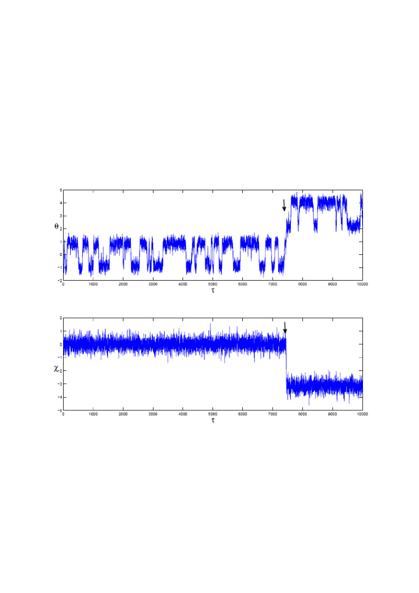
The Langevin equations (11),(12) describe the random motion of the ’particle’ with coordinates ($\theta$, $\chi$) in the periodic potential (13), which is a set of bistable cells (eight-shaped contours in Fig. 3a). We have numerically integrated these stochastic equations by Ito’s method (see e.g. [9]) for different values of parameter $\alpha$ and the strength of the fluctuations $D$. The typical traces of $\theta(\tau)$ and $\chi(\tau)$ are shown in Fig. 4. They correspond to random motion in bistable potential, Fig. 3. The arrows indicate the switching from one unit cell in Fig. 3a to another. With knowledge of $\theta(\tau)$ and $\chi(\tau)$ the average circulating current in the ring is obtained as:

$$I(\phi_{e})=I_{c}<<sin(\chi+\theta)>>.$$ (14)

The averaging $<<...>>$ includes for each value of flux $\phi_{e}$ the average over time of traces ($\theta(\tau),\chi(\tau)$) and the average over set of 50 traces.

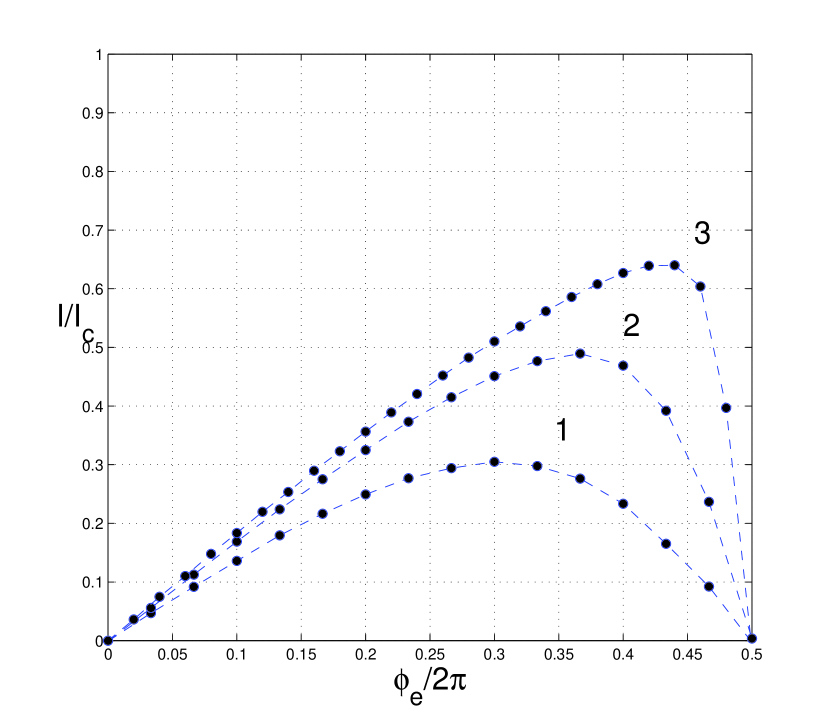
The calculated in such way the current-flux curves for different values of $D$ and different values of parameter $\alpha$ are presented in Fig. 5 and Fig. 6.

From Eqs. (11-13) the Fokker-Plank equation for distribution function $P(\chi,\theta)$ can be reconstructed:

$$\frac{\partial P}{\partial\tau}=\frac{\partial}{\partial\chi}(\frac{\partial U}{\partial\chi}P)+\frac{D}{2}\frac{\partial^{2}}{\partial\chi^{2}}P+\frac{1}{1+2\alpha}\frac{\partial}{\partial\theta}(\frac{\partial U}{\partial\theta}P)+\frac{1}{2}\frac{3D}{(1+2\alpha)^{2}}\frac{\partial^{2}}{\partial\theta^{2}}P$$ (15)

The Fokker-Plank equation (15) admits the stationary potential solution (see [9]) in the special case $\alpha=1$, i.e. when all three junctions are identical. For $\alpha=1$ the analytical solution reads:

$$P=\frac{e^{-\frac{2}{D}U(\chi,\theta)}}{\textsl{N}},$$ (16)

$$\textsl{N}=\int\int d\chi d\theta e^{-\frac{2}{D}U(\chi,\theta)}$$ (17)

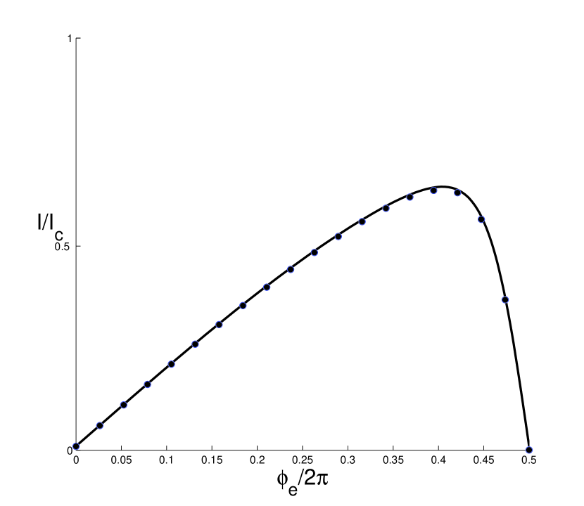
Since the potential $U$ is $2\pi$ periodical function of variables $\chi$ and $\theta$ the average current in the ring is:

$$\frac{I}{I_{c}}=\frac{\int^{2\pi}_{0}\int^{2\pi}_{0}d\chi d\theta sin(\chi+\theta)e^{-\frac{2}{D}U(\chi,\theta)}}{\int^{2\pi}_{0}\int^{2\pi}_{0}d\chi d\theta e^{-\frac{2}{D}U(\chi,\theta)}}$$ (18)

In Fig. 7 we compare the numerical results (circles) and the $I(\phi_{e})$ obtained from the analitical formula (18) (solid line) for the case $\alpha=1$ and $D=0.2$. This comparison was used as an additional calibration of our numerical procedure, which is working at arbitrary values of $\alpha$.

3 The probing of qubit’s state in classical and quantum modes.

As we wrote in introduction we probe a qubit with making use of a tank circuit by the impedance measurement technique [10]. It was convincingly shown [10, 11] that the observable phase difference $\delta(\varphi_{e})$ between tank current $I_{rf}$ and tank voltage $V_{rf}$ both in classical and quantum modes reads:

$$\tan\delta(\varphi_{e})\approx\Theta\frac{dI}{d\varphi_{e}},$$ (19)

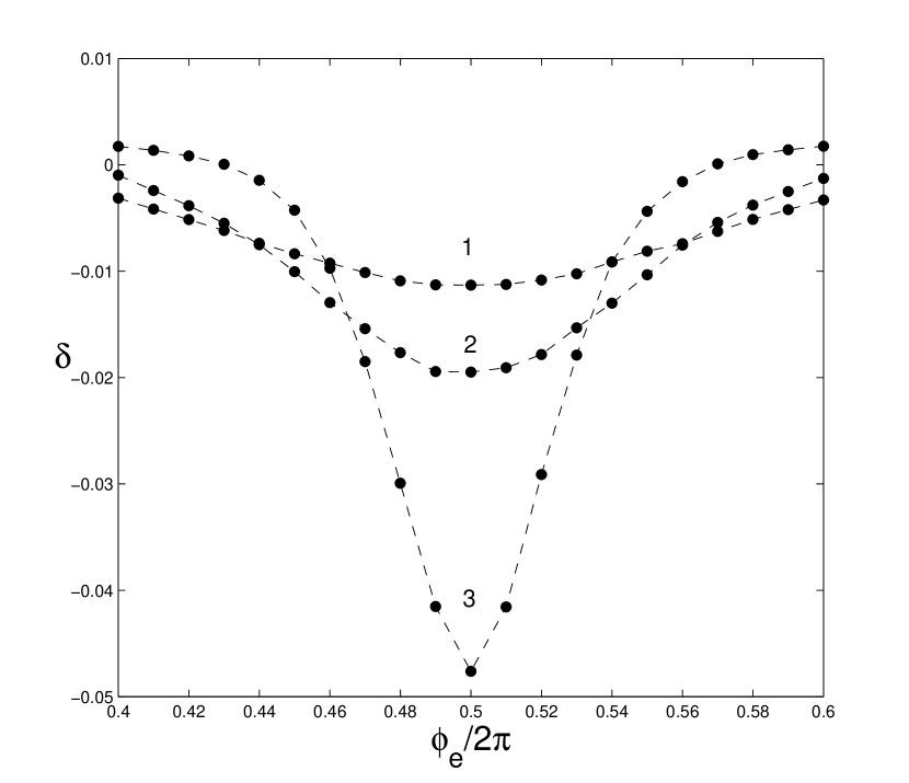
where $\Theta$ is const, which characterizes the inductive coupling of the qubit with the tank circuit. By using the results of Section 2 we calculated output signal $\delta(\varphi_{e})$ for classical noise affected mode. For different levels of noise $D$ (all of those correspond to nonhysteretic regime) the dependencies $\delta(\varphi_{e})$ are shown in Fig. 8.

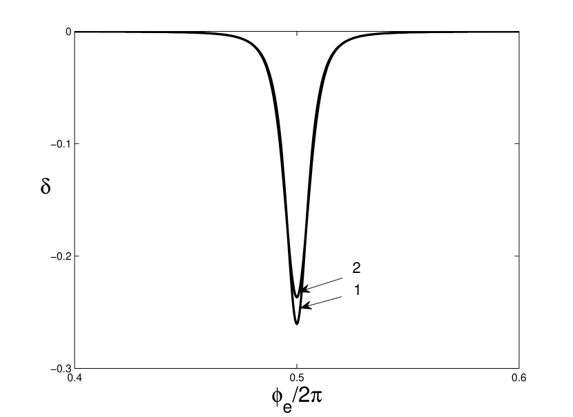
In the quantum noise free mode (see Appendix A) the nonhysteretic behavior is achieved by the tunneling between two wells. The phase shift $\delta(\varphi_{e})$ in this case is described by Eqs. (19,22). It is presented in Fig. 8 for the same as in the classical case value of the qubit-tank coupling constant $\Theta$ and experimentally realized qubit’s parameters $I_{p}\Phi_{0}=200GHz,\Delta=1.5GHz$.

Comparing classical and quantum modes (Figs. 8,9) we have found that in quantum mode the dip on the $\delta(\varphi_{e})$ dependence remains constant at wide temperature range $kT\leq\Delta$. This reflects the fact that tunneling splitting $\Delta$ does not depend on the temperature. The depth of the dip is changed with temperature - excitations to the upper level depress the value of the average qubit’s current. For classical mode the situation is rather different. First of all for reasonable set of qubit parameters it is impossible to get such narrow and profound dip similar to obtained in quantum mode. Moreover, the temperature dependence of $\delta(\varphi_{e})$ dip demonstrates that its width strongly depends on $T$. Therefore by analyzing the temperature dependence of $\delta(\varphi_{e})$ one can easily distinguish between quantum and classical modes.

In conclusion we analyzed the temperature dependence of imaginary part of impedance for three-junction loop-tank circuit arrangement in quantum and classical modes. We argued that impedance for these modes have quite different temperature dependencies and, therefore, can be easily distinguished experimentally.

Appendix A Quantum mode of a flux qubit

Since the tunnel splitting in flux qubit is much smaller than the difference between upper energy levels, qubits are effectively two-level quantum systems. In the two level approximation a flux qubit can be described by the pseudo-spin Hamiltonian

$$H(t)=-\Delta\sigma_{\!x}-\varepsilon\sigma_{\!z}\;,$$ (20)

where $\sigma_{x},\sigma_{z}$ are the Pauli matrices; $\Delta$ is the tunneling amplitude. The qubit bias is given by $\varepsilon=I_{p}\Phi_{0}f_{e}$, where $I_{p}$ is the magnitude of the qubit persistent current and $f_{e}=\Phi_{e}/\Phi_{0}-1/2$. The stationary energy levels can be easily found from the Hamiltonian (20):

$$E_{\pm}(\varepsilon)=\pm\sqrt{\varepsilon^{2}+\Delta^{2}},$$ (21)

and the average value of the qubit current at temperature $T$ is:

$$I(\varepsilon)=\frac{\varepsilon I_{p}}{\sqrt{\varepsilon^{2}+\Delta^{2}}}\tanh\frac{\sqrt{\varepsilon^{2}+\Delta^{2}}}{kT},$$ (22)

Note, that the dependence (21) is valid within the narrow interval of $\Phi_{e}$ near $\Phi_{e}=\Phi_{0}/2$, where the potential $U$ (13) is bistable.

FIGURE CAPTIONS
Figure 1. $\phi(\phi_{e})$ for rf SQUID in nonhysteretic and hysteretic modes
Figure 2. The scheme of persistent current (flux) qubit
Figure 3. a. Contour plot of the potential $U(\theta,\chi)$ (13), $\alpha=0.8$. b. Bistable potential profile along line 1-2 in Fig3a at $\phi_{e}=\pi$,$\alpha=0.8$.
Figure 4. The random motion of phases $\theta$ and $\chi$ in bistable potential (Fig.3b) for $\phi_{e}=\pi$,$\alpha=0.8$ and $D=0.1$
Figure 5. The dependences $I(\phi_{e})$ for $\alpha=0.8$ and $D=0.5(1),D=0.25(2),D=0.1(3)$
Figure 6. The dependences $I(\phi_{e})$ for $D=0.1$ and $\alpha=0.5(1),\alpha=0.8(2),\alpha=1(3)$
Figure 7. The comparision of numerical (circles) and analitical (solid line) calculations. $D=0.2$, $\alpha=1$
Figure 8. The phase shift $\delta(\varphi_{e})$ in classical mode. $\alpha=0.8$ and $D=0.3(1),D=0.2(2),D=0.1(3)$
Figure 9. The phase shift $\delta(\varphi_{e})$ in quantum mode. $T/\Delta=0.1(1),T/\Delta=1(2)$

Figure 1: $\phi(\phi_{e})$ for rf SQUID in nonhysteretic and hysteretic modes

Figure 2: The scheme of persistent current (flux) qubit

Figure 3: a. Contour plot of the potential $U(\theta,\chi)$ (13), $\alpha=0.8$. b. Bistable potential profile along line 1-2 in Fig3a at $\phi_{e}=\pi$,$\alpha=0.8$.

Figure 4: The random motion of phases $\theta$ and $\chi$ in bistable potential (Fig.3b) for $\phi_{e}=\pi$,$\alpha=0.8$ and $D=0.1$

Figure 5: The dependences $I(\phi_{e})$ for $\alpha=0.8$ and $D=0.5(1),D=0.25(2),D=0.1(3)$

Figure 6: The dependences $I(\phi_{e})$ for $D=0.1$ and $\alpha=0.5(1),\alpha=0.8(2),\alpha=1(3)$

Figure 7: The comparision of numerical (circles) and analitical (solid line) calculations. $D=0.2$, $\alpha=1$

Figure 8: The phase shift $\delta(\varphi_{e})$ in classical mode. $\alpha=0.8$ and $D=0.3(1),D=0.2(2),D=0.1(3)$

Figure 9: The phase shift $\delta(\varphi_{e})$ in quantum mode. $T/\Delta=0.1(1),T/\Delta=1(2)$

References

- [1] A. Barone and G. Paterno, Physics and applications of the Josephson effect, Wiley, New York, 1982.
- [2] V.A. Khlus and I.O. Kulik, Sov. Tech. Phys. Lett. 20, 283, 1975.
- [3] L.D. Jackel, R.A. Buhrman, and W.W. Webb, Phys. Rev. B 10, 2782 (1974).
- [4] E. Il’ichev, V. Zakosarenko, V. Schultze, H.-G. Meyer, H.E. Hoenig, V.N. Glyantsev, A. Golubov, Appl. Phys. Lett. 72, 731 (1998)
- [5] R.de Bruyn Ouboter and A.N. Omelyanchouk, Physica B 216, 37 (1995).
- [6] E. Il’ichev, V. Zakosarenko, R.P.J. IJsselsteijn, V. Schultze, JLTP 106, N.3/4, 503, (1997).
- [7] E. Il’ichev, V. Zakosarenko, V. Schultze, H.E. Hoenig, H.-G. Meyer, K.O. Subke, H. Burkhard, M. Schilling, Appl. Phys. Lett. 76, 100, (2000).
- [8] J.E. Mooij, T.P. Orlando, L. Levitov, L. Tian, C.H. van der Wal, and S. Lloyd, Science 285, 1036 (1999).
- [9] C.W.Gardiner Handbook of stochastic methods, 2nd ed.,Shpringer, Berlin, 1990.
- [10] E. Il’ichev, N. Oukhanski, Th. Wagner, H.-G. Meyer, A.Yu. Smirnov, M. Grajcar, A. Izmalkov, D. Born, W. Krech, and A. Zagoskin, Low Temp. Phys., 30, 620, (2004).
- [11] S.N. Shevchenko, cond-mat/0708.0464