From planes to spheres:
About gravitational lens magnifications

Abstract

We discuss the classic theorem according to which a gravitational lens always produces at least one image with a magnification greater than unity. This theorem seems to contradict the conservation of total flux from a lensed source. The standard solution to this paradox is based on the exact definition of the reference ‘unlensed’ situation, in which the lens mass can either be removed or smoothly redistributed.

We calculate magnifications and amplifications (in photon number and energy flux density) for general lensing scenarios not limited to regions close to the optical axis. In this way the formalism is naturally extended from tangential planes for the source and lensed images to complete spheres. We derive the lensing potential theory on the sphere and find that the Poisson equation is modified by an additional source term that is related to the mean density and to the Newtonian potential at the positions of observer and source. This new term generally reduces the magnification, to below unity far from the optical axis, and ensures conservation of the total photon number received on a sphere around the source.

This discussion does not affect the validity of the focusing theorem, in which the unlensed situation is defined to have an unchanged affine distance between source and observer. The focusing theorem does not contradict flux conservation, because the mean total magnification (or amplification) directly corresponds to different areas of the source (or observer) sphere in the lensed and unlensed situation. We argue that a constant affine distance does not define an astronomically meaningful reference.

By exchanging source and observer, we confirm that magnification and amplification differ according to Etherington’s reciprocity law, so that surface brightness is no longer strictly conserved. At this level we also have to distinguish between different surface brightness definitions that are based on photon number, photon flux, and energy flux.

1 Introduction

Already Einstein (1936) calculated the magnification of a background star lensed by a foreground compact mass and found the classic result for the total magnification of both images, which decreases for large impact angles (far away from the optical axis) but always stays above unity.

At that time, gravitational lensing was regarded as a theoretical curiosity with very little chance of leading to observable effects. Much later, after the first actual lens systems had been found, Schneider (1984) presented and proved a theorem stating that a gravitational lens with arbitrary mass distribution will always produce at least one image with a magnification greater than 1. Since the theorem is thought to be valid for all configurations of source, lens and observer, one might naively think that this necessarily leads to an increase of the total number of photons from the source. This would be in contradiction with the fact that lensing can neither create nor destroy photons. It was already pointed out by Schneider (1984) that such an interpretation is not correct. In order to compare the lensed with the unlensed situation, it is essential to define the latter in a meaningful way, which is far from trivial. In general relativity, the lens will slightly distort the geometry of the whole Universe, so that it is plainly impossible to add a lens without changing the configuration of source and observer. The ‘reference situation’ in the standard explanation is the one in which the mass of the lens is redistributed evenly over the Universe. It can be shown that the comparison finds no net increase of photon number then (e.g. Weinberg, 1976). The reason for this is that two differently lensed scenarios are compared.

Some level of uneasiness remained in the minds of several authors, because one may think of situations in which the general validity of the theorem would still lead to a violation of photon number conservation. Avni & Shulami (1988) calculated the amplification caused by a point-mass lens by dropping the small-angle approximation of light rays with respect to the optical axis (defined by observer and lens), which is generally used in the standard formalism. One might think that far from the optical axis the deflection becomes so weak that the full calculation would add only higher-order terms which are not relevant in the end. Still, slightly surprising, these authors find that the amplification actually sinks below 1, which corrects for the amplification excess close to the optical axis. Avni & Shulami (1988) worked with a point-mass metric in Schwarzschild coordinates, and fixed the radial coordinate relative to the lens for the comparison of lensed and unlensed situation. Schneider et al. (1992) question the value of such a comparison. They argue that there is generally no unique way to compare mean fluxes in different space-times. Nevertheless, approximating the calculations of Avni & Shulami (1988) for regions close to the optical axis would directly lead to the tangential plane approach of Schneider (1984). It is not entirely clear why (if at all) the theorem loses its validity far from the optical axis.

Jaroszyński & Paczyński (1996) make similar calculations, but keep the metric distance between source and observer constant for the comparison. They find that the effect of the lens changes the total area of the sphere around the source and can thus (without contradicting photon conservation) lead to changes in the averaged amplification. They also make a distinction between magnification and amplification, which becomes relevant at the accuracy levels required far from the optical axis.

None of these publications actually presents the magnification to second order (in terms of the deflection potential) for arbitrary angles to the optical axis. They either approximate for small angles or include only first-order terms. One aim of our work is to extend the calculations to include second-order terms also for large impact angles. Even more important is the discussion of appropriate unlensed situations to act as a reference in order to define magnifications and amplifications.

We will also develop the formalism to treat off-axis lenses similarly to the standard small-angle approximation and learn which part of the proof of the magnification theorem cannot be generalised for this situation. This will be done for arbitrary mass distributions and not only for point-mass lenses.

The outline of this paper is as follows. We start in Sec. 2 with a brief review of the standard planar lensing theory, which is described in a tangential plane at the position of the lens. This includes the magnification theorem and a simple version of its proof. In Sec. 3 we explain our approach of discussing the apparent magnification in terms of solid angles. In this way we can avoid the explicit definition of an unlensed reference situation. Solid angle must always integrate to $4\pi$, so that the magnification theorem (in these terms) cannot hold everywhere. This discussion is equivalent to a reference situation in which the area of the source sphere stays constant.

Section 4.1 comprises calculations for a point-mass lens at infinity. We explicitly find that the magnification sinks below 1 far from the optical axis. General mass distributions (still with source at infinity) are discussed in Sec. 4.2. There we develop the potential theory of lenses on the sphere as an extension of the standard potential theory in the tangential plane. We find that the Poisson equation is modified by an additional source term, which ensures the validity of Gauss’ theorem on the closed sphere.

The exact form of magnification matrices on the sphere for finite (and possibly large) deflection angles is investigated in Appendix B. For our current discussion we only need the result that the magnification matrix in terms of second-order derivatives of the potential differs from the usual form only to second order in the deflection angle, so that this difference can be neglected.

In Sec. 5 we extend our calculations to finite values of the source distance and explicitly calculate deflection angles and magnifications for point-mass lenses. By adapting the potential theory to this situation, we find that the correction terms in Poisson equation and magnification are directly related to the Newtonian potential at the source and observer.

The subject of reciprocity is covered in Sec. 6, where we exchange the role of source and observer to relate magnification with amplification. These two are not the same anymore, so that the surface brightness is no longer conserved if we define it in a standard physical sense. This is a direct consequence of the reciprocity theorem of Etherington (1933) and of the space-time modification at the position of source and observer, caused by the gravitational field of the lens. In anticipation of this result we try to make a clear distinction between amplification and magnification from the beginning.

After a brief discussion of light travel times in Sec. 7 we summarise and discuss our results in Secs. 8 and 9.

2 Planar lensing theory

2.1 Basics

Here we only recall the most relevant aspects. The complete theory can be found elsewhere (e.g. Schneider et al., 1992). Close to an optical axis (which can be defined arbitrarily, conventionally by observer and lens centre), the geometry of a gravitational lens system can be projected on the tangential plane of the celestial sphere. This leads to the notion of the source plane for the true source structure and the lens or image plane for the observed lensed image(s). In these planes we define two-dimensional unit-less vectors which are based on angular coordinates on the sphere. We now restrict the discussion to static, ‘thin’ lenses, where the light is deflected only very close to the lens plane. We can then interpret the action of the lens as a potential time-delay, which affects the light when it crosses the lens plane. This direct potential delay causes a deflection and thus changes the geometrical light path, which creates an additional geometrical delay. The total delay $\Delta t$ is usually written in terms of the Fermat potential, which comprises the geometrical and potential parts in a normalized version:

$$\phi_{\mn@boldsymbol{\theta}_{\text{s}}}(\mn@boldsymbol{\theta})=\frac{(\mn@boldsymbol{\theta}-\mn@boldsymbol{\theta}_{\text{s}})^{2}}{2}-\psi(\mn@boldsymbol{\theta})$$ (1)

$$\Delta t=\frac{D_{\smash{\text{d}}}D_{\smash{\text{s}}}}{c\,D_{\smash{\text{ds}}}}\phi_{\mn@boldsymbol{\theta}_{\text{s}}}$$ (2)

Here the vectors of the observed image and true source position are $\mn@boldsymbol{\theta}=(\theta_{x},\theta_{y})$ and $\mn@boldsymbol{\theta}_{\text{s}}$, respectively. The distance parameters are angular-size distances between observer and lens/source ($D_{\smash{\text{d}}}$, $D_{\smash{\text{s}}}$) and between lens and observer ($D_{\smash{\text{ds}}}$). For simplicity, we assume that the lens is embedded in a global Minkowski metric. In a cosmological situation, Eq. (2) would have to be scaled by a redshift factor $1+z_{\text{d}}$, but remains valid apart from that.

We define the apparent deflection angle $\mn@boldsymbol{\alpha}$ to fulfil the lens equation

$$\mn@boldsymbol{\theta}_{\text{s}}=\mn@boldsymbol{\theta}-\mn@boldsymbol{\alpha}(\mn@boldsymbol{\theta})\hskip 5.0pt\text{.}$$ (3)

Deflection and time-delay are related by Fermat’s theorem: Images form at stationary points of the time-delay function. These can be minima, maxima or saddle-points. Critical images with degenerate Hessian matrix (see below, e.g. Einstein rings of point sources) are unstable and shall not be discussed here. We thus take the derivative of the Fermat potential in Eq. (1) and substitute the lens equation (3) to find that the deflection angle is the gradient of the potential,

$$\mn@boldsymbol{\alpha}(\mn@boldsymbol{\theta}) =\mn@boldsymbol{\nabla}\psi(\mn@boldsymbol{\theta})\hskip 5.0pt\text{.}$$ (4)

If we calculate the potential from the mass distribution, we can prove that it obeys a Poisson equation

$$\mn@boldsymbol{\nabla}^{2}\psi(\mn@boldsymbol{\theta}) =2\kappa(\mn@boldsymbol{\theta})\hskip 5.0pt\text{.}$$ (5)

The convergence $\kappa$ is the projected surface mass density $\Sigma$ in units of the critical density

$$\Sigma_{\text{c}} =\frac{c^{2}}{4\pi G}\frac{D_{\smash{\text{s}}}}{D_{\smash{\text{d}}}D_{\smash{\text{ds}}}}\hskip 5.0pt\text{.}$$ (6)

In more detail, we can express the Hessian matrix, consisting of the second-order derivatives of $\psi$, in terms of the convergence and the two-dimensional external shear $\mn@boldsymbol{\gamma}=(\gamma_{x},\gamma_{y})$:

$${\textbf{{H}}}=\begin{pmatrix}\psi_{xx}&\psi_{xy}\\ \psi_{yx}&\psi_{yy}\end{pmatrix}=\begin{pmatrix}\kappa+\gamma_{x}&\gamma_{y}\\ \gamma_{y}&\kappa-\gamma_{x}\end{pmatrix}$$ (7)

2.2 The magnification theorem

This theorem was presented by Schneider (1984) and is described in a broader context by Schneider et al. (1992). Here we only want to make a plausibility proof, without claiming to be fully mathematically rigorous. The local magnification matrix M is the inverse Jacobian of the lens mapping, Eq. (3):

$${\textbf{{M}}}^{-1}=\frac{\partial\mn@boldsymbol{\theta}_{\text{s}}}{\partial\mn@boldsymbol{\theta}}={\textbf{{1}}}-{\textbf{{H}}}$$ (8)

The scalar magnification $\mu$ is the determinant of this matrix,

$$\mu^{-1}=\det\left({\textbf{{1}}}-{\textbf{{H}}}\right)=(1-\kappa)^{2}-\gamma^{2}\hskip 5.0pt\text{,}$$ (9)

with $\gamma=|\mn@boldsymbol{\gamma}|$. The sign of $\mu$ defines the parity of the image.

For large $\mn@boldsymbol{\theta}$, the Fermat potential will be dominated by the first term in Eq. (1) for all realistic mass distributions, i.e. it grows quadratically with $\mn@boldsymbol{\theta}$. Local mass concentrations will produce minima in $\psi$ that can diverge for point masses, but can not lead to positive discontinuous peaks in $\psi$. It is thus plausible that at least one local minimum of $\phi$ exists. This point is a solution of the lens equation and corresponds to a real image. Being a minimum, the Hessian of the Fermat potential, ${\textbf{{1}}}-{\textbf{{H}}}$, must be positive definite. The eigenvalues can be easily derived to be $1-\kappa\pm\gamma$, which must thus both be positive. If we add the condition that the convergence or density $\kappa$ is non-negative, we find $0<\mu^{-1}<1$. In other words, this image has positive parity and a magnification $\mu>1$. As a result, the total magnification of all images corresponding to one source position is always greater than unity.

The fact that lensing increases the observed flux density in all directions, no matter where the lens is positioned, raises the question how this can be consistent with conservation of total flux. This issue is discussed by Schneider (1984), Schneider et al. (1992) and references therein. The basic argument is that one has to thoroughly define the unlensed situation, relative to which the magnifications are calculated. Adding a lens modifies the geometry of the Universe, so that the comparison is not trivial. This can be illustrated by a thought experiment in which we shrink the size of the Universe by some factor. This would move all sources closer to all observers, so that they would all see an increased flux density. Still, there is of course no contradiction with energy or flux conservation at all.

An important example for total net magnifications is the case of a point-mass lens, where the calculations were presented long before the general theorem (Einstein, 1936; Refsdal, 1964). The total magnification of the two images as a function of the angular separation $\theta_{\text{s}}$ between lens and source is given by the standard expression

$$\mu_{\text{tot}}=\frac{\theta_{\text{s}}^{2}+2m}{\theta_{\text{s}}\sqrt{\theta_{\text{s}}^{2}+4m}}\hskip 5.0pt\text{,}$$ (10)

which is greater than unity everywhere. Here we have defined

$$m=\frac{4GM}{c^{2}}\frac{D_{\smash{\text{ds}}}}{D_{\smash{\text{d}}}D_{\smash{\text{s}}}}\quad\to\quad\frac{4GM}{c^{2}\,D_{\smash{\text{d}}}}\quad\text{(for $D_{\smash{\text{s}}}\gg D_{\smash{\text{d}}},D_{\smash{\text{ds}}}\approx D_{\smash{\text{s}}}$),}$$ (11)

which is the square of the Einstein radius. We can calculate the excess magnification by integrating over the tangential plane:

$$\Delta\mu =\iint\text{d}^{2}\theta_{\text{s}}\,(\mu_{\text{tot}}-1)=2\pi\,m$$ (12)

The order of magnitude of this excess is plausible, because the lens produces significant additional magnifications (of the order 1) over a region corresponding to the Einstein ring with radius $\sqrt{m}$.

We will later find that the solution of the magnification paradox has to do with terms of $\mu^{-1}$ that are linear in the deflection. This can be anticipated by the fact that the excess in Eq. (12) is also linear in $m$. Counting only the terms linear in the deflection (linear in $\psi$, $\kappa$, $\gamma$) of Eq. (9), we find

$$\mu^{-1}\approx 1-H_{xx}-H_{yy}=1-\mn@boldsymbol{\nabla}^{2}\psi=1-2\kappa\hskip 5.0pt\text{.}$$ (13)

The first-order magnification can only be reduced below 1 if either $\kappa$ is negative or the Poisson equation is modified in an appropriate way. We do expect the latter to happen when we leave the tangential plane and consider the sphere. The divergence (source density) of the deflection field $\mn@boldsymbol{\nabla}\!\cdot\mn@boldsymbol{\alpha}=\mn@boldsymbol{\nabla}^{2}\psi$ cannot be positive everywhere, because of Gauss’ law. There simply is no chance for the flux of $\mn@boldsymbol{\alpha}$ to escape from the closed sphere, so that the integrated divergence must vanish.

3 Solid angles

To avoid most of the complications of arbitrary definitions for reference situations, we want to interpret the apparent paradox in a different way. Instead of discussing fluxes, we want to investigate how solid angles are mapped from the observed image sphere to the true source sphere, which we put at an infinite distance, where the metric perturbation by the lens can be neglected. Using solid angles instead of areas on the source sphere, we can avoid a possible scaling of the total area. The total solid angle always remains $4\pi$.

We do not restrict the discussion to small regions around the optical axis (corresponding to the tangential plane) but instead allow for arbitrary impact angles.

3.1 Conservation of solid angle

We start by integrating the total apparent solid angle on the image sphere and transform this into an integral over the source sphere. For this we assume that all lines of sight end somewhere on the source sphere and that every part of the source sphere can be seen in at least one direction, i.e. we neglect possible horizons which would add higher order corrections.

$$4\pi=\oint\text{d}\Omega(\mn@boldsymbol{\theta})=\oint\text{d}\Omega_{\text{s}}(\mn@boldsymbol{\theta}_{\text{s}})\,\mu_{\text{tot}}(\mn@boldsymbol{\theta}_{\text{s}})$$ (14)

$$\mu_{\text{tot}}(\mn@boldsymbol{\theta}_{\text{s}})=\sum_{\mn@boldsymbol{\theta}(\mn@boldsymbol{\theta}_{\text{s}})}\bigl{|}\mu(\mn@boldsymbol{\theta})\bigr{|}=\sum_{\mn@boldsymbol{\theta}(\mn@boldsymbol{\theta}_{\text{s}})}\left|\frac{\text{d}\Omega}{\text{d}\Omega_{\text{s}}}(\mn@boldsymbol{\theta})\right|$$ (15)

The sum is taken over all images corresponding to the respective source position. We learn that the total magnification, defined in terms of solid angle elements, averaged over the source sphere must be equal to unity. Even if it is valid close the the optical axis, the magnification theorem cannot hold in other regions where the excess has to be compensated.

We conclude that if the magnification theorem would hold in this situation, we would have a real paradox that had to be taken seriously. We will learn later that the magnification theorem does indeed become invalid for large impact angles. In these regions the primary image is only very weakly deflected. Any additional images will be strongly deflected (invalidating the weak-deflection approximation), but highly demagnified. In the following discussion we will mostly neglect these images, which allows us to consider the magnification as a function of image positions instead of the total magnification as a function of source position. Fig. 3 shows that this simplification is justified.

Figure 1: Deflected lines of sight with the observer in the centre and the source sphere as circle. The vertical line defines the optical axis, the hatched circle shows the lens. The regularly spaced dots on the source sphere label the corresponding image positions (straight projections of the lines of sight).

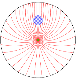
Figure 1 illustrates why the magnification theorem can be valid around the optical axis but not everywhere. We see that the lens increases the density of lines of sight on the source sphere around the (forward) optical axis, corresponding to a magnification greater than unity. On the tangential plane, this would be possible everywhere, because lines of sight (or solid angle on the sky) can be ‘borrowed from infinity’. In contrast to this, the total solid angle must be conserved on the compact sphere. This necessarily leads to magnifications less than unity somewhere, seen in the lower parts of the diagram. Note that, for simplicity, a lens without multiple imaging is shown here. The lens mass distribution was chosen in such a way that the magnifications can be seen already in this two-dimensional cross-sectional view. Generally the density of lines of sight only shows in the full three-dimensional geometry.

3.2 Reference situations and the refraction analogue

We now know that for solid angles, measured for sources at infinity, the magnification theorem cannot hold. However, we have to be very specific about the situations that are compared to define a magnification. The magnification according to Eq. (15) defines the ratio of solid angles of a cone of light rays measured by the observer and at infinity. In astronomy we are interested in the ratio of solid angles of one and the same source seen with and without the action of the lens. Naively, one would define the unlensed reference situation in such a way that the distance between observer and source is kept constant, but distances are not uniquely defined in a curved space-time so that this approach is not unique. The picture of solid angles and a very large source sphere can also be interpreted as a reference situation in which the total area of the source sphere is the same in the lensed and unlensed situation. Flux conservation then demands a mean magnification of unity, so that general validity of the magnification theorem cannot be expected.

We want to postpone the discussion of an appropriate reference situation by redefining the problem. It is well-known that the gravitational light deflection can be described as the action of a refractive medium that fills an Euclidean space, whose coordinates are identified with those used in the standard form of the weak-field metric equation (16). In this model, the unlensed situation would obviously be the one with all distances unchanged but the refractive medium removed. Solid angles can then directly be identified with areas on the source sphere, so that the reasoning about solid angles in Sec. 3.1 inevitably leads to a failure of the magnification theorem in this situation. Since this contradicts the result of Sec. 2, even though the formalism is exactly the same, we have to identify and abandon the inadmissible assumptions or approximations. Once the formalism has been generalised, we can come back to the definition of reference situations.

As an alternative to refraction we can refer to the Newtonian picture of the deflection of massive particles moving with the speed of light. Modulo a factor of 2, the deflection follows exactly the same law as in general relativity, but the geometry of space and time are not altered.

4 Sources at infinite distances

4.1 Point-mass lens

We know that close to the optical axis the magnification theorem holds. From the discussion of Fig. 1, we expect that it breaks down at larger impact angles. Therefore we have to generalize the usual formalism to allow source positions far from the lens centre. However, we will keep the weak-field approximation so that deflection angles still have to be small.

We describe the lens(es) as small perturbation of an asymptotic Minkowski metric instead of a more realistic Robertson-Walker metric. This simplifies the treatment without obscuring the apparent magnification paradox or its solution. We use the static weak-field metric in isotropic coordinates, so that locally observed angles (and solid angles) can be derived directly from the spatial coordinates $\mn@boldsymbol{r}=(x,y,z)$. In terms of the Newtonian potential $\Psi$, the line element can be written as

$$\text{d}s^{2}=\left(1+\frac{2\Psi}{c^{2}}\right)c^{2}\text{d}t^{2}-\left(1-\frac{2\Psi}{c^{2}}\right)\text{d}\mn@boldsymbol{r}^{2}\hskip 5.0pt\text{.}$$ (16)

This leads to the geodesic equation for light in first order approximation

$$\ddot{\mn@boldsymbol{r}}=-2\frac{\dot{\mn@boldsymbol{r}}^{2}}{c^{2}}\mn@boldsymbol{\mn@boldsymbol{\nabla}_{\!\!\perp}}\Psi\hskip 5.0pt\text{,}$$ (17)

where $\mn@boldsymbol{\mn@boldsymbol{\nabla}_{\!\!\perp}}$ denotes the transversal part (relative to $\dot{\mn@boldsymbol{r}}$) of the gradient, and dots stand for derivatives with respect to the affine parameter. Within first order (in $\Psi$), the geometrical length or local time can also be used equivalently.

4.1.1 Deflection angle

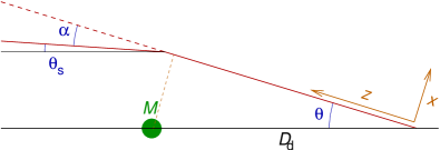
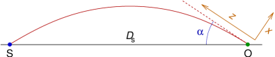
We want to calculate the deflection angle of a point mass $M$ with a source at infinity. We restrict ourselves to the plane defined by lens, source and observer, which contains the complete light ray. The coordinates have their origin at the observer, $z$ is measured along the unperturbed line of sight, $x$ in the perpendicular direction (Fig. 2). The deflection angle is defined according to the standard form of the lens equation (3). The lens, located at

$$x_{0}=-D_{\smash{\text{d}}}\sin\theta\hskip 5.0pt\text{,}\quad z_{0}=D_{\smash{\text{d}}}\cos\theta\hskip 5.0pt\text{,}$$ (18)

produces a Newtonian potential of

$$\Psi(x,z)=-\frac{GM}{\sqrt{(x-x_{0})^{2}+(z-z_{0})^{2}}}\hskip 5.0pt\text{.}$$ (19)

The deflection angle is calculated by integrating Eq. (17) along the unperturbed line of sight. It is defined to be positive for deflection in the negative $z$-direction. We use $z$ as affine parameter:

$$\alpha =-\Delta\dot{x}=-\int_{0}^{\infty}\text{d}z\,\ddot{x}(x=0,z)$$ (20)

$$=\frac{2}{c^{2}}\int_{0}^{\infty}\text{d}z\,\nabla_{\!\!\perp}\Psi(x=0,z)$$ (21)

$$=-\frac{2GM}{c^{2}}\,x_{0}\int_{0}^{\infty}\text{d}z\,\Bigl{[}x_{0}^{2}+(z-z_{0})^{2}\Bigr{]}^{-3/2}$$ (22)

$$=-\frac{2GM}{c^{2}}\frac{1+z_{0}\bigl{(}x_{0}^{2}+z_{0}^{2}\bigr{)}^{-1/2}}{x_{0}}$$ (23)

$$=\frac{m}{2}\frac{1+\cos\theta}{D_{\smash{\text{d}}}\,\sin\theta}=\frac{m}{2}\cot\frac{\theta}{2}$$ (24)

In the limit of small $\theta$, i.e. close to the optical axis, we recover the standard result $\alpha=m/\theta$, with the definition of $m$ from Eq. (11).

Figure 2: Geometry of the light deflection with a source at infinity. The angles $\theta$, $\theta_{\text{s}}$ and $\alpha$ are positive in our sign convention. Here and in all following geometrical considerations, we pretend that space is Euclidean (and space-time Minkowski) and treat the light deflection as a non-geometrical effect. The figures represent the geometry of the coordinates used to define the metric in Eq. (16). Isotropy of the metric ensures that all angles correspond to real locally observable angles. Straight lines in the figures are not necessarily geodesics in real space or space-time.

Note that for large $\theta$ the deflection is not confined to regions small compared to $D_{\smash{\text{d}}}$, but takes place over a range $\sim|x_{0}|$. This means that not even the point-mass lens can be considered as thin anymore.

4.1.2 Potential

The deflection angle in Eq. (24) can be written as the derivative of a potential $\psi$, which is defined on the sphere as

$$\psi_{\text{pm}}(\theta)=m\ln\sin\frac{\theta}{2}=\frac{m}{2}\ln(1-\cos\theta)+\text{const}\hskip 5.0pt\text{.}$$ (25)

Figure 3: Magnification of both images (positive and negative parity) and the total magnification as a function of the source position for a lens of $m=(1^{\prime\prime})^{2}=2.35\cdot 10^{-11}$. For small angles (left), the magnification is indistinguishable from the classic result. Far from the optical axis (right), the magnification approaches $1-m/2$ instead of 1. The magnification theorem does not hold in this region. The total magnification and the magnification of only the positive parity image are indistinguishable for very large impact angles. This justifies our approach of not discussing the total magnification of all images but only that of the primary image ($\mu_{+}$).

4.1.3 Magnification

Consider as source a thin concentric annulus around the lens, as seen by the observer. With radius $\theta_{\text{s}}$ and width $\text{d}\theta_{s}$, the solid angle is $\text{d}\Omega_{\text{s}}=2\pi\sin\theta_{\text{s}}\,\text{d}\theta_{\text{s}}$. This annulus will be observed at radius $\theta$ with width $\text{d}\theta$ and solid angle $\text{d}\Omega=2\pi\sin\theta\,\text{d}\theta$. We separate the magnification into the tangential and radial parts, $M_{\text{T}}$ and $M_{\text{R}}$, respectively:

$$\mu^{-1} =\frac{\text{d}\Omega_{\text{s}}}{\text{d}\Omega}=M_{\text{T}}^{-1}M_{\text{R}}^{-1}$$ (26)

$$M_{\text{T}}^{-1} =\frac{\sin\theta_{\text{s}}}{\sin\theta}=\frac{\sin(\theta-\alpha)}{\sin\theta}=\cos\alpha-\cot\theta\sin\alpha$$ (27)

$$M_{\text{R}}^{-1} =\frac{\text{d}\theta_{\text{s}}}{\text{d}\theta}=1-\frac{\text{d}\alpha}{\text{d}\theta}$$ (28)

$$=1+\frac{m}{4}\sin^{-2}\frac{\theta}{2}$$ (29)

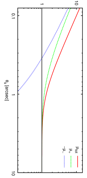
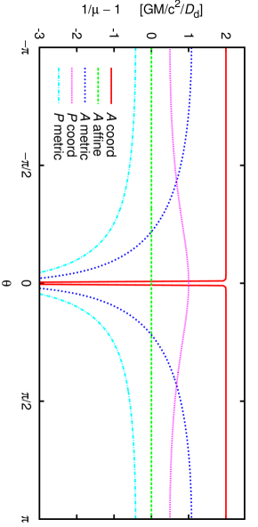
The magnification we get from Eqs. (26–28) with the deflection angle from Eq. (24) is plotted in Fig. 3. The deflection angle and its derivative are correct only to first order in $m$, so that the first order is also sufficient for the radial and tangential magnifications. Up to this order, we find

$$M_{\text{T}}^{-1} =1-\alpha\cot\theta\hskip 5.0pt\text{,}$$ (30)

$$\mu^{-1} =1+\frac{m}{2}-\frac{m^{2}}{4}\frac{\cos\theta}{(1-\cos\theta)^{2}}\hskip 5.0pt\text{.}$$ (31)

For large $\theta$, the $m/2$ term in Eq. (31) is dominant, whilst in the normal lensing regime, the $m^{2}$ term becomes more important. Expanded in powers of $\theta$, we find

$$\mu^{-1}=1+\frac{m}{2}-\frac{m^{2}}{\theta^{4}}\Bigl{[}1+{\cal O}\bigl{(}\theta^{2}\bigr{)}\Bigr{]}\hskip 5.0pt\text{.}$$ (32)

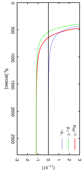
The corrections in the small-angle regime (last term) are not relevant in our context. The isotropic correction $m/2$, on the other hand, leads to violations of the magnification theorem. Far away from the optical axis, the magnification sinks below unity. The transition region with a magnification of 1 is around $\theta=\sqrt[4]{2m}$, approximately the square root of the Einstein radius. For typical galaxy lensing cases, this is a few arc-minutes from the lens, far away from the strong-lensing regime but still at a small angle. For microlensing, the transition region is even closer.

The small correction of the order $m$ ($10^{-10}$ in typical galaxy scale lenses) is completely irrelevant for all practical calculations. Nevertheless, this term is responsible for the conservation of total flux or solid angle. Integrated over the complete celestial sphere, it leads to a deficit of $2\pi\,m+{\cal O}(m^{2})$, which exactly compensates for the excess found in Eq. (12). Because the modification is of first order in $m$, the following discussion will concentrate on first-order effects.

4.2 General mass distributions on the sphere

4.2.1 Potential

Knowing the potential for a point-mass lens from Eq. (25), we can easily generalize for arbitrary mass distributions, defined by the three-dimensional mass density $\rho(\mn@boldsymbol{r})$:

$$\psi(\mn@boldsymbol{\theta}) =\frac{4G}{c^{2}}\iiint\text{d}^{3}r^{\prime}\,\frac{\rho(\mn@boldsymbol{r}^{\prime})}{r^{\prime}}\ln\sin\frac{\measuredangle(\mn@boldsymbol{\theta},\mn@boldsymbol{r}^{\prime})}{2}$$ (33)

$$=\frac{2G}{c^{2}}\iiint\text{d}^{3}r^{\prime}\,\frac{\rho(\mn@boldsymbol{r}^{\prime})}{r^{\prime}}\ln\left(1-\frac{\mn@boldsymbol{\theta}\cdot\mn@boldsymbol{r}^{\prime}}{r^{\prime}}\right)+\text{const}$$ (34)

The direction is denoted by the unit vector $\mn@boldsymbol{\theta}$ with $\mn@boldsymbol{r}=\mn@boldsymbol{\theta}r$. We separate the radial integration from the tangential part on the sphere by introducing the normalized surface mass density

$$\sigma(\mn@boldsymbol{\theta})=\frac{4\pi G}{c^{2}}\int_{0}^{\infty}\text{d}r\,r\,\rho(\mn@boldsymbol{r})$$ (35)

to find

$$\psi(\mn@boldsymbol{\theta})=\frac{1}{2\pi}\oint\text{d}\Omega^{\prime}(\mn@boldsymbol{\theta}^{\prime})\,\sigma(\mn@boldsymbol{\theta}^{\prime})\,\ln\left(1-\mn@boldsymbol{\theta}\cdot\mn@boldsymbol{\theta}^{\prime}\right)+\text{const}\hskip 5.0pt\text{.}$$ (36)

In the tangential plane, this corresponds to the integral

$$\psi(\mn@boldsymbol{\theta})=\frac{1}{\pi}\iint\text{d}^{2}\theta^{\prime}\,\sigma(\mn@boldsymbol{\theta}^{\prime})\,\ln|\mn@boldsymbol{\theta}-\mn@boldsymbol{\theta}^{\prime}|+\text{const}\hskip 5.0pt\text{.}$$ (37)

Even though this formalism is valid for arbitrary mass distributions, it is correct only to first order in $\rho$. This means it cannot be used for multi-plane strong lensing, where the change of impact parameter in one lens plane as a result of the deflection in another plane becomes relevant.

4.2.2 Poisson equation

The Poisson equation for the spherical potential $\psi$ can be derived with very little formal calculations. We determine the flux $F$ of the deflection field $\mn@boldsymbol{\alpha}$ through a circle of radius $\theta$ around the point mass $m$, corresponding to $\sigma(\mn@boldsymbol{\theta})=\pi\,m\,\delta^{2}(\mn@boldsymbol{\theta})$. This is the product of $\alpha$ with the circumference of the circle,

$$F(\theta)=\alpha(\theta)\;2\pi\sin\theta=\pi m(1+\cos\theta)\hskip 5.0pt\text{.}$$ (38)

In the limit of $\theta\to 0$, this starts with $F(0+)=2\pi m$ and then decreases linearly with the enclosed area $A$ of the circle:

$$F(\theta) =2\pi m-\frac{m}{2}A(\theta) A(\theta) =2\pi(1-\cos\theta)$$ (39)

We know from Gauss’ theorem that this flux equals the integrated divergence of the field ($=$ Laplacian of the potential), so that we can write the Poisson equation as

$$\mn@boldsymbol{\nabla}^{2}\psi_{\text{pm}}(\mn@boldsymbol{\theta})=2\pi\,m\,\delta^{2}(\mn@boldsymbol{\theta})-\frac{m}{2}\hskip 5.0pt\text{.}$$ (40)

The $\delta$ term is the same as on the tangential plane. The mass acts in the usual way as source for the deflection field. However, in contrast to the tangential plane, the sphere is closed, so that sources and sinks of the field must compensate each other; the field lines cannot extend to infinity. Without the second term in Eq. (40), the field lines would continue and meet at $\theta=\pi$ where they would form an additional singularity of mass $-m$. Instead, the field ‘decays’ to ensure a vanishing total integrated $\mn@boldsymbol{\nabla}^{2}\psi$.

For an arbitrary mass distribution $\sigma$, the Poisson equation reads

$$\mn@boldsymbol{\nabla}^{2}\psi(\mn@boldsymbol{\theta})=2\left[\sigma(\mn@boldsymbol{\theta})-\overline{\sigma}\right]=:2\kappa(\mn@boldsymbol{\theta})\hskip 5.0pt\text{.}$$ (41)

We learn that not $\sigma$ itself is the source of the field but the difference of $\sigma$ and the mean surface mass density

$$\overline{\sigma}=\frac{1}{4\pi}\oint\text{d}\Omega(\mn@boldsymbol{\theta})\,\sigma(\mn@boldsymbol{\theta})\hskip 5.0pt\text{.}$$ (42)

In Appendix A.1 we show how the spherical lensing potential can be written directly as integral over the Newtonian potential. It is the three-dimensional Poisson equation that leads to the first term in Eq. (41). The second term is related to the Newtonian potential at the position of the observer. This tells us that the deviations from the standard formalism can be related to local distortions of space-time.

4.2.3 The magnification matrix

The (inverse) magnification matrix is given by the Jacobian of the lens mapping. On the tangential plane, the Jacobian of Eq. (3) leads directly to the Hessian of the potential, see Eq. (8). The situation is more complicated on the curved sphere, where finite displacements cannot be treated as vectors. In Appendix B we calculate the magnification matrix for arbitrary deflection functions $\mn@boldsymbol{\alpha}(\mn@boldsymbol{\theta})$, including large deflection angles. In terms of this section, where the deflection angle $\mn@boldsymbol{\alpha}$ is the gradient of a potential $\psi$, the exact magnification matrix from Eq. (104) can be written in coordinates $(\parallel,\perp)$ parallel and perpendicular to the negative deflection angle $-\mn@boldsymbol{\alpha}$, as

$${\textbf{{M}}}^{-1}=\begin{pmatrix}1-\psi_{\parallel;\parallel}&&-\psi_{\parallel;\perp}\\[6.45831pt] -\psi_{\perp;\parallel}\dfrac{\sin\alpha}{\alpha}&&\cos\alpha-\psi_{\perp;\perp}\dfrac{\sin\alpha}{\alpha}\end{pmatrix}\hskip 5.0pt\text{.}$$ (43)

The lower indices of $\psi$ denote the second-order (covariant) derivatives with respect to the coordinate axes. The corrections in $\cos\alpha$ and $\sin\alpha/\alpha$ are of second order in the deflection $\alpha$. These terms can be set to unity if the magnification matrix is needed only to first order. The result is then equivalent to the planar formalism in Eqs. (7–8), but with the modified spherical potential.

For a point mass at a distance $\theta$, the Hessian of $\psi$ is diagonal with

$$\psi_{\parallel;\parallel}=\psi_{\theta,\theta}\hskip 5.0pt\text{,}\qquad\psi_{\perp;\perp}=\psi_{\theta}\cot\theta\hskip 5.0pt\text{,}$$ (44)

which leads to

$${\textbf{{M}}}^{-1}=\begin{pmatrix}1+\dfrac{m}{4}\sin^{-2}\dfrac{\theta}{2}&&0\\[6.45831pt] 0&&\cos\alpha-\cot\theta\sin\alpha\end{pmatrix}\hskip 5.0pt\text{.}$$ (45)

This matrix corresponds exactly to Eqs. (27–29). Neglecting the curvature terms in ${\textbf{{M}}}^{-1}$ corresponds to the linear approximation in Eq. (30–31), where only the term linear in $\alpha$ was included for the tangential magnification.

4.2.4 Magnification theorem

We have now, to first order, derived the magnification matrix as the Hessian matrix of a potential, analogously to the standard formalism. We can thus formally follow the proof for the magnification theorem as described in Sec. 2.2 step by step. However, the assumption of positive (effective) $\kappa$ is no longer true, see Eq. (41), so that we cannot infer magnifications greater than unity from the signs of the eigenvalues. Even though the density (even in comparison with the reference situation) is still strictly non-negative, the convergence is not, which invalidates one of the assumptions for the proof of the theorem.

Recall that, in order to define a firm foundation for this reasoning, we refered to non-relativistic situations with unperturbed geometry in which the deflection is caused either by refraction or by Newtonian deflection. If we now return to the relativistic scenario but define the infinitely large source sphere in such a way that the area is the same for the lensed and unlensed situation, we come to exactly the same conclusion for that case.

5 Sources at finite distances

In the following we allow for sources at finite distances. In this situation, the metric on the source sphere is modified by the lens, so that the previously used approach is not possible anymore, but assumptions about the unlensed reference situation have to be made. We do this by fixing the coordinate distances, which would also be the appropriate approach for the model of refraction or Newtonian deflection in an Euclidean metric. Modifications of the results for different conventions (like fixed metric distances) will be discussed later.

Main aim of this section is the analysis of lens deflection and the potential theory on the sphere as opposed to the planar theory. For completeness this has to be generalised to finite distances. Most of the discussion of the magnification theorem, on the other hand, is based on the case of sources at infinity, because some arbitrariness in defining a reference situation can be avoided then.

Figure 4: The apparent deflection angle $\alpha$ is defined as the difference between the apparent and true source position. Changes of the direction of the light path will therefore affect $\alpha$ scaled with $D_{\smash{\text{ds}}}(z)/D_{\smash{\text{s}}}$.

5.1 Deflection angle

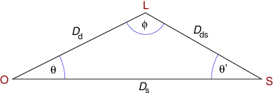
If the source is at a finite distance $D_{\smash{\text{s}}}$ from the observer, the simple geometry in Fig. 2 has to be modified. If we want to keep the form of the lens equation (3), the apparent deflection angle $\mn@boldsymbol{\alpha}$ is no longer defined as the angle between the incoming and outgoing light ray, but as the difference between apparent and true source position (Fig. 4). In the thin-lens approximation, this leads to the well-known correction factor of $D_{\smash{\text{ds}}}/D_{\smash{\text{s}}}$ to transform the true to the apparent deflection angle. As mentioned earlier, far from the optical axis not even the point-mass lens can be considered as being thin, which means that $D_{\smash{\text{ds}}}$ is not defined globally. If we instead consider how a local change of $\dot{x}$ in Eqs. (20) and following affects the difference between true and apparent source position, we find that the integrands have to be scaled with the local $D_{\smash{\text{ds}}}(z)/D_{\smash{\text{s}}}=(D_{\smash{\text{s}}}-z)/D_{\smash{\text{s}}}$. In addition, the integration has to end at $z=D_{\smash{\text{s}}}$. With the same approach as before ($\lambda=z$), we find for the deflection angle of a point-mass lens

$$\alpha(\theta) =-\int_{0}^{D_{\smash{\text{s}}}}\text{d}z\,\frac{D_{\smash{\text{s}}}-z}{D_{\smash{\text{s}}}}\,\ddot{x}(x=0,z)$$ (46)

$$=-\frac{2GM}{c^{2}}\,x_{0}\int_{0}^{D_{\smash{\text{s}}}}\text{d}z\,\frac{D_{\smash{\text{s}}}-z}{D_{\smash{\text{s}}}}\,\Bigl{[}x_{0}^{2}+(z-z_{0})^{2}\Bigr{]}^{-3/2}$$ (47)

$$=-\frac{2GM}{c^{2}}\,\frac{1}{x_{0}D_{\smash{\text{s}}}}\left[\frac{(D_{\smash{\text{s}}}-z_{0})^{2}+x_{0}^{2}}{\sqrt{\smash[b]{x_{0}^{2}+(D_{\smash{\text{s}}}-z_{0})^{2}}}}+\frac{z_{0}(D_{\smash{\text{s}}}-z_{0})-x_{0}^{2}}{\sqrt{\smash[b]{x_{0}^{2}+z_{0}^{2}}}}\right]$$ (48)

$$=\frac{2GM}{c^{2}}\,\frac{D_{\smash{\text{ds}}}(\theta)+D_{\smash{\text{s}}}\cos\theta-D_{\smash{\text{d}}}}{D_{\smash{\text{d}}}D_{\smash{\text{s}}}\sin\theta}\hskip 5.0pt\text{,}$$ (49)

with the coordinate distance between source and mass

$$D_{\smash{\text{ds}}}(\theta)=\sqrt{D_{\smash{\text{s}}}^{2}+D_{\smash{\text{d}}}^{2}-2D_{\smash{\text{d}}}D_{\smash{\text{s}}}\cos\theta}\hskip 5.0pt\text{.}$$ (50)

In the limit of small $\theta$ this reduces to

$$\alpha=\frac{4GM}{c^{2}}\left[\frac{D_{\smash{\text{s}}}-D_{\smash{\text{d}}}}{D_{\smash{\text{d}}}D_{\smash{\text{s}}}}\,\frac{\operatorname{\Theta}(D_{\smash{\text{s}}}-D_{\smash{\text{d}}})}{\theta}+{\cal O}(\theta)\right]\hskip 5.0pt\text{.}$$ (51)

For a source behind the lens, we recover the classical limiting case with the appropriate scaling of the apparent deflection angle. If the lens is further away than the source (which we may call background lensing), the singularity at $\theta=0$ vanishes and the deflection generally becomes much weaker, just as expected. In this case the maximum effect will be reached at some finite $\theta$.

Note that in contrast to the standard expressions, Eq. (49) is valid for all combinations of distances. Even $D_{\smash{\text{s}}}\approx D_{\smash{\text{d}}}$ is possible, including the limit of self-lensing with $D_{\smash{\text{s}}}=D_{\smash{\text{d}}}$.

Figure 5: Definition of the distance parameters $D_{\smash{\text{d}}}$, $D_{\smash{\text{s}}}$, $D_{\smash{\text{ds}}}$ and the angles $\theta$, $\theta^{\prime}$, and $\phi$ for a compact lens at L. Observer and source are denoted by O and S. Recall that, in concordance with our general philosophy, the lengths and angles are in our convention defined in an Euclidean metric with the same coordinates as in the general metric of Eq. (16). (See caption of Fig. 2.)

5.2 Magnification

Later we will compare magnification with amplification, which corresponds to an exchange of observer and source, i.e. $\theta\leftrightarrow\theta^{\prime}$ and $D_{\smash{\text{d}}}\leftrightarrow D_{\smash{\text{ds}}}$ (see Fig. 5). For this purpose, we formulate the magnification in a form that explicitly shows the symmetries. We use the trigonometric relations

$$D_{\smash{\text{s}}}^{2}=D_{\smash{\text{d}}}^{2}+D_{\smash{\text{ds}}}^{2}-2D_{\smash{\text{d}}}D_{\smash{\text{ds}}}\cos\phi\hskip 5.0pt\text{,}$$ (52)

$$\hbox to0.0pt{$D_{\smash{\text{s}}}\sin\theta$\hss}\phantom{D_{\smash{\text{s}}}\cos\theta}=D_{\smash{\text{ds}}}\sin\phi\hskip 5.0pt\text{,}$$ (53)

$$D_{\smash{\text{s}}}\cos\theta=D_{\smash{\text{d}}}-D_{\smash{\text{ds}}}\cos\phi\hskip 5.0pt\text{,}$$ (54)

to write the tangential magnification $M_{\text{T}}$ following Eq. (30) for the deflection angle in Eq. (49) as

$$M_{\text{T}}^{-1} =1+\frac{GM}{c^{2}}\left(\frac{1}{D_{\smash{\text{d}}}}-\frac{1}{D_{\smash{\text{ds}}}}-\frac{D_{\smash{\text{d}}}+D_{\smash{\text{ds}}}}{D_{\smash{\text{d}}}D_{\smash{\text{ds}}}}\tan^{2}\frac{\phi}{2}\right)\hskip 5.0pt\text{.}$$ (55)

The radial magnification can be determined from the derivative of the deflection angle, see Eq. (28),

$$M_{\text{R}}^{-1} =1+\frac{GM}{c^{2}}\left(\frac{1}{D_{\smash{\text{d}}}}-\frac{1}{D_{\smash{\text{ds}}}}+\frac{D_{\smash{\text{d}}}+D_{\smash{\text{ds}}}}{D_{\smash{\text{d}}}D_{\smash{\text{ds}}}}\tan^{2}\frac{\phi}{2}\right)\hskip 5.0pt\text{.}$$ (56)

To first order in M, the scalar magnification is given by

$$\mu^{-1}\approx 1+\frac{2GM}{c^{2}}\left(\frac{1}{D_{\smash{\text{d}}}}-\frac{1}{D_{\smash{\text{ds}}}}\right)\hskip 5.0pt\text{.}$$ (57)

Note that for these calculations we assumed that the coordinates of source and observer are the same in the lensed and unlensed situation. For finite $D_{\smash{\text{s}}}$, the lens will modify the geometry of the source sphere, which makes the definition of the unlensed reference geometry somewhat arbitrary. While coordinates can be fixed for point-like sources, this is not appropriate for the components of extended sources. For those, we should keep their physical size constant to allow for a meaningful comparison.

From the metric in Eq. (16) we infer that the ratio of area to solid angle (on the source sphere) changes isotropically with the potential $\Psi_{\text{s}}$ at the source position:

$$\text{d}A_{\text{s}}=\left(1-\frac{2\Psi_{\text{s}}}{c^{2}}\right)D_{\smash{\text{s}}}^{2}\,\text{d}\Omega_{\text{s}}$$ (58)

Using this we can define the true area magnification $\mu_{(A)}$ as a function of the solid angle magnification $\mu_{(\Omega)}$, which we called $\mu$ before:

$$\mu_{(\Omega)}^{-1} =\frac{\text{d}\Omega_{\text{s}}}{\text{d}\Omega} \mu_{(A)}^{-1} =\frac{1}{D_{\smash{\text{s}}}^{2}}\frac{\text{d}A_{\text{s}}}{\text{d}\Omega}=\left(1-\frac{2\Psi_{\text{s}}}{c^{2}}\right)\mu_{(\Omega)}^{-1}$$ (59)

The radial and tangential magnifications $M_{\text{R}}$ and $M_{\text{T}}$ both have to be corrected with the same factor, which is the square root of that for the scalar magnification, so that

$$\frac{{M_{\text{R}}}_{(A)}^{-1}}{{M_{\text{R}}}_{(\Omega)}^{-1}}=\frac{{M_{\text{T}}}_{(A)}^{-1}}{{M_{\text{T}}}_{(\Omega)}^{-1}}=1-\frac{\Psi_{\text{s}}}{c^{2}}=1+\frac{GM}{c^{2}}\frac{1}{D_{\smash{\text{ds}}}}\hskip 5.0pt\text{.}$$ (60)

We now apply this correction to the magnifications from Eqs. (55–56):

$${M_{\text{T}}}_{(A)}^{-1} =1+\frac{GM}{c^{2}}\left(\frac{1}{D_{\smash{\text{d}}}}-\frac{D_{\smash{\text{d}}}+D_{\smash{\text{ds}}}}{D_{\smash{\text{d}}}D_{\smash{\text{ds}}}}\tan^{2}\frac{\phi}{2}\right)$$ (61)

$${M_{\text{R}}}_{(A)}^{-1} =1+\frac{GM}{c^{2}}\left(\frac{1}{D_{\smash{\text{d}}}}+\frac{D_{\smash{\text{d}}}+D_{\smash{\text{ds}}}}{D_{\smash{\text{d}}}D_{\smash{\text{ds}}}}\tan^{2}\frac{\phi}{2}\right)$$ (62)

The first-order scalar magnification is

$$\mu_{(A)}^{-1}\approx 1+\frac{2GM}{c^{2}}\frac{1}{D_{\smash{\text{d}}}}\hskip 5.0pt\text{.}$$ (63)

All these magnifications refer to an unlensed situation with the same coordinate distance to the source. As alternatives we discuss fixed affine and metric distances in Appendix C.

5.3 Potential and Poisson equation

The potential can be derived by integrating the point-mass deflection angle in Eq. (49), or alternatively by integrating over the appropriately scaled three-dimensional potential $\Psi$, as shown in Appendix A.3 with the result in Eq. (95).

In Appendix A.2 we derive the Poisson equation by integrating over the three-dimensional potential derivatives, and find the relation

$$\mn@boldsymbol{\nabla}^{2}\psi(\mn@boldsymbol{\theta})=2\sigma(\mn@boldsymbol{\theta})+2\frac{\Psi_{\text{o}}-\Psi_{\text{s}}(\mn@boldsymbol{\theta})}{c^{2}}\hskip 5.0pt\text{,}$$ (64)

where $\Psi_{\text{o}}$ is the Newtonian potential at the observer. The projected surface mass density is now defined as

$$\sigma(\mn@boldsymbol{\theta})=\frac{4\pi G}{c^{2}}\int_{0}^{D_{\smash{\text{s}}}}\text{d}r\,r\frac{D_{\smash{\text{s}}}-r}{D_{\smash{\text{s}}}}\,\rho(\mn@boldsymbol{r})\hskip 5.0pt\text{.}$$ (65)

The weight function in Eq. (65) has the shape of a parabola with maximum at $r=D_{\smash{\text{s}}}/2$ and zeros at $r=0$ and $r=D_{\smash{\text{s}}}$. However, since the apparent size of a mass clump scales with $1/r^{2}$, the influence of a mass element at $r$ is proportional to $1/r-1/D_{\smash{\text{s}}}$.

In classical lensing theory, the divergence of the deflection angle leads to the local surface mass density. Far away from the optical axis but for sources at infinity, this is changed in the way that we obtain in Eq. (41) the density contrast relative to the mean density, which results from the gravitational potential at the position of the observer (see Appendix A.1). Now we find in Eq. (64) for finite $D_{\smash{\text{s}}}$ that the divergence is also affected by the potential at the source position (see Appendix A.2). These two contributions describe the influence of all masses, while the surface mass density only includes masses inside of the source sphere. The projected surface mass density $\sigma$ vanishes completely for $D_{\smash{\text{s}}}\leq D_{\smash{\text{d}}}$, i.e. in the case where the source is closer to the observer than the lens.

We recall from Sec. 2.2 that the divergence of the deflection is directly related to the first-order scalar magnification. The same is true here, but the corresponding magnification now refers to solid angles instead of area. When writing Eq. (64) for the point-mass, we find that the potential terms lead directly to the correction terms in Eq. (57) if we follow the same recipe as in Eq. (13).

As consistency check we should test if the integral over Eq. (64) vanishes, as required by the compact geometry of the sphere. We know from Gauss’ theorem that the potential of a homogeneous spherical shell is equivalent to that of a point-mass for regions outside of the shell, and constant inside. We can turn the argument around, to learn that the potential averaged over the surface of any sphere is the same as that in the centre of the sphere, if masses are located only outside of the sphere. These masses do not influence the integral of the difference $\Psi_{\text{o}}-\Psi_{\text{s}}$ in Eq. (64). For masses inside of the sphere, on the other hand, the averaged potential is independent of their location, so that the total mass can be thought of as being in the centre:

$$<\Psi_{\text{s}}> =-G\oint\text{d}\Omega\int_{0}^{D_{\smash{\text{s}}}}\text{d}r\,r^{2}\frac{\rho(\mn@boldsymbol{r})}{D_{\smash{\text{s}}}} +C$$ (66)

$$\Psi_{\text{o}} =-G\oint\text{d}\Omega\,\int_{0}^{D_{\smash{\text{s}}}}\text{d}r\,r^{2}\frac{\rho(\mn@boldsymbol{r})}{r} +C$$ (67)

The contributions from masses outside of the sphere are denoted as $C$. By comparison with Eq. (65), we find

$$<\Psi_{\text{o}}-\Psi_{\text{s}}> =-c^{2}<\sigma>\hskip 5.0pt\text{.}$$ (68)

As required, the average source density in Eq. (64) vanishes.

Note that for $D_{\smash{\text{s}}}\gg D_{\smash{\text{d}}}$ all expression in this section (and in Appendix A.2–A.3) converge to the ones for infinite $D_{\smash{\text{s}}}$ derived in the previous sections and Appendix A.1. The distinction between $\mu_{(A)}$ and $\mu_{(\Omega)}$ is not necessary in this limit.

6 Reciprocity and surface brightness

The magnifications in Eqs. (61–63) are not invariant under the exchange of source and observer. Writing $\mu_{(A)}(\text{o},\text{s})=\mu_{(A)}$ for the magnification of the source as seen by the observer and $\mu_{(A)}(\text{s},\text{o})$ for the magnification of the observer as seen by the source, we find (by exchanging $D_{\smash{\text{d}}}\leftrightarrow D_{\smash{\text{ds}}}$) the following relation, which is correct up to first-order terms in the tangential and radial magnifications.

$$\frac{\mu_{(A)}(\text{s},\text{o})}{\mu_{(A)}(\text{o},\text{s})}=1+\frac{2GM}{c^{2}}\left(\frac{1}{D_{\smash{\text{d}}}}-\frac{1}{D_{\smash{\text{ds}}}}\right)$$ (69)

What does this mean physically? The magnification $\mu_{(A)}(\text{o},\text{s})$ defines the scaling of the apparent size of a magnified source as seen by the observer. The reciprocal $\mu_{(A)}(\text{s},\text{o})$, on the other hand, is inversely proportional to the area in the observer plane that is spanned by a certain light bundle; that means it defines the amplification in terms of the number of photons received from the source by the observer per detector area element.

The ratio of amplification to magnification in Eq. (69) provides the gravitational change of ‘surface brightness’, measured as photon number density per solid angle. In this sense, gravitational lensing does not conserve surface brightness.

This may seem surprising but is in perfect agreement with the reciprocity theorem derived by Etherington (1933). If one defines in an arbitrary space-time for two events $x$ and $y$, which are connected by a null-geodesic, i.e. one can be seen by the other, the angular size distances $D_{xy}$ for the distance of $y$ as seen by $x$ and vice versa, it can be shown that the two are related by

$$\frac{D_{yx}}{D_{xy}}=\frac{1+z_{y}}{1+z_{x}}\hskip 5.0pt\text{,}$$ (70)

where $z$ are the redshifts as measured by an arbitrary observer.

In our situation, the lens magnifications act as corrections to obtain the effective angular size distances from $D_{\smash{\text{s}}}$:

$$\frac{1}{D_{\text{os}}^{2}} =\frac{\mu_{(A)}(\text{o},\text{s})}{D_{\smash{\text{s}}}^{2}} \frac{1}{D_{\text{so}}^{2}} =\frac{\mu_{(A)}(\text{s},\text{o})}{D_{\smash{\text{s}}}^{2}}$$ (71)

The gravitational redshifts produced by the field of the lens can be derived from the metric, Eq. (16), as

$$1+z =\left.\frac{c\,\text{d}t}{\text{d}s}\right|_{\text{d}\mn@boldsymbol{r}=0}=1-\frac{\Psi}{c^{2}}=1+\frac{GM}{c^{2}}\frac{1}{D}$$ (72)

for a point mass at a distance $D$.

We can confirm Eq. (69) by taking the ratio of Eqs. (71) and inserting Eq. (70) and the redshifts from Eq. (72):

$$\frac{\mu_{(A)}(\text{s},\text{o})}{\mu_{(A)}(\text{o},\text{s})} =\frac{D_{\text{os}}^{2}}{D_{\text{so}}^{2}}=\left(\frac{1+z_{\text{o}}}{1+z_{\text{s}}}\right)^{2}=\left(\frac{1+\dfrac{GM}{c^{2}}\dfrac{1}{D_{\smash{\text{d}}}}}{1+\dfrac{GM}{c^{2}}\dfrac{1}{D_{\smash{\text{ds}}}}}\right)^{2}$$ (73)

$$=1+\frac{2GM}{c^{2}}\left(\frac{1}{D_{\smash{\text{d}}}}-\frac{1}{D_{\smash{\text{ds}}}}\right)$$ (74)

So far, we have discussed the surface brightness defined as photon number per solid angle. If we want to determine it in terms of energy flux density $F$, we have to take into account that both the energy of the individual photons and the arrival rate at the observer are affected by the redshift. This provides another factor of $(1+z_{\text{o}})^{2}/(1+z_{\text{s}})^{2}$, so that the surface brightness in terms of intensity scales with

$$\frac{F_{\text{obs}}}{F_{0}}=\left(\frac{1+z_{\text{o}}}{1+z_{\text{s}}}\right)^{4}=1+\frac{4GM}{c^{2}}\left(\frac{1}{D_{\smash{\text{d}}}}-\frac{1}{D_{\smash{\text{ds}}}}\right)\hskip 5.0pt\text{.}$$ (75)

The scaling of the surface brightness with $(1+z)^{-4}$ is, of course, a well-known fact in cosmology. Here we have exactly the same effect, but caused by the metric perturbations of a gravitational lens at finite distance. In any case, we should keep in mind that the effect is extremely small, typically of the order $m$ or the square of the Einstein radius. For typical galaxy-scale lenses with Einstein radii of the order $\sim 1^{\prime\prime}$ this corresponds to $\sim 10^{-11}\mbox{--}10^{-10}$.

7 Light travel time

We separate the light travel time into three parts: The undisturbed travel time $D_{\smash{\text{s}}}/c$, and the geometrical and potential parts of the time-delay, $\Delta t_{\text{geom}}$ and $\Delta t_{\text{pot}}$, respectively. The potential part is easy to calculate. We start with the metric from Eq. (16) and write the (coordinate) time interval for a null-curve along the $z$-axis as

$$\text{d}t=\left(1-\frac{2\Psi}{c^{2}}\right)\frac{\text{d}z}{c}\hskip 5.0pt\text{.}$$ (76)

For a point-mass lens, the integral is basically the same as for the metric distance shown in Appendix C.2:

$$\Delta t_{\text{pot}} =\int\text{d}t-\frac{D_{\smash{\text{s}}}}{c}=-\frac{2}{c^{3}}\int_{0}^{D_{\smash{\text{s}}}}\text{d}z\,\Psi(x=0,z)$$ (77)

$$=\frac{2GM}{c^{3}}\ln\frac{D_{\smash{\text{ds}}}(\theta)+D_{\smash{\text{d}}}+D_{\smash{\text{s}}}}{D_{\smash{\text{ds}}}(\theta)+D_{\smash{\text{d}}}-D_{\smash{\text{s}}}}+\text{const}$$ (78)

We observe that this is proportional to the deflection potential in Eq. (25) only in the limit $D_{\smash{\text{s}}}\to\infty$, where we have $\Delta t_{\text{pot}}=-D_{\smash{\text{d}}}\,\psi/c$. In the general case there is no proportionality to Eq. (95).

In fact, we do not expect a one-to-one relation between $\Delta t_{\text{pot}}$ and the potential $\psi$ as in the case of thin lenses. The argument used in Sec. 2.1 to explain why the deflection angle is proportional to the gradient of the potential time-delay breaks down, because the geometrical part of the time-delay does not keep its simple form of Eq. (1). It cannot be expressed in terms of image and source position alone anymore, because the deflection is not restricted to a lens plane (or sphere). In order to determine the geometrical delay, we have to know the full three-dimensional mass distribution and not just its projection $\sigma$ or the projected deflection potential $\psi$.

Because it cannot be easily generalized for arbitrary mass distributions, we do not present the calculation of $\Delta t_{\text{geom}}$ for a point-mass lens.

Figure 6: Plots of several first-order magnifications defined in different ways for a point-mass lens. Labels $A$ refer to area magnification, $P$ to photon number amplification. Different distances are held constant for the comparison with the unlensed situation: coordinate distance, affine distance and metric distance. For ‘$A$ coord’, we added the second-order magnification calculated for $GM/D_{\smash{\text{d}}}/c^{2}=10^{-8}$, which has no noticeable effect for $D_{\smash{\text{s}}}<D_{\smash{\text{d}}}$. left: $D_{\smash{\text{s}}}=3D_{\smash{\text{d}}}$, right: $D_{\smash{\text{s}}}=D_{\smash{\text{d}}}/3$

8 Summary

We discuss the classical magnification paradox in gravitational lensing in order to better understand if and how a magnification greater than unity everywhere can be consistent with global photon number conservation. It is of fundamental importance to allow for large angles relative to the optical axis. Therefore we develop a formalism of lens and source spheres instead of planes. In this situation, even a point-mass lens cannot be regarded as a thin lens anymore. The ‘thickness’ of a lens is not defined by the extent of the mass distribution but by the extent of the deflecting potential and its derivatives. The thickness of a point-mass lens is thus closely related to the impact parameter and can be of the same order of magnitude as the distances involved.

To avoid ambiguities, we start by considering a source at infinity, so that the geometry on the source sphere is not changed by the action of the lens, and the area of the source sphere is not modified. This makes a comparison with the unlensed situation meaningful. We calculate magnifications by mapping solid angle elements from the lens sphere to the source sphere. Because we do not include horizons around black holes, which are corrections at higher order, the total solid angle of the whole sky must be $4\pi$ with and without lensing. Lensing defines a one-to-many mapping from the source sphere to the lens sphere. We see the background sky in all directions, no parts of the background are hidden, but some parts may be multiply imaged. With this argument, we conclude that the total magnification cannot be larger than unity for all positions on the source sphere, in contradiction to the magnification theorem. This thought is supported by a simple geometric argument. The density of deflected lines of sight on the source sphere (or equivalently light rays on an observer’s sphere around the source) can be increased close to the optical axis, because a lens with positive mass has a focusing tendency. In the approximation of the tangential plane, this can be true everywhere, since lines of sight (and solid angle elements) can be borrowed from infinity. Once we consider the complete sphere, this is no longer possible. Solid angle elements that are moved towards the optical axis must be re-moved from other parts of the sphere. The magnification cannot be larger than one everywhere. For this argument it is essential to work with solid angles on a source sphere at infinity. With a sphere at finite distance, the area density of projected lines of sight can well increase everywhere, simply by making the area of the sphere smaller. Masses modify the geometry, so that mean magnifications above one are no longer paradoxical. The further the source sphere moves away, the weaker these distortions get. For a finite mass, they decrease without limits and can finally be neglected.

The non-relativistic pictures of refraction and Newtonian deflection in unperturbed geometry support this view. In these scenarios a paradox cannot be avoided if no corrections to the formalism are made.

With this motivation, we calculate the deflection angle for a point-mass lens for arbitrary angles to the optical axis with source at infinity and derive magnifications from that. We find an additional first-order term that lowers the magnification, violates the magnification theorem at some point, and assures total conservation of solid angle. In order to understand which part of the classical proof of the theorem becomes invalid once we go from tangential planes to full spheres, we develop the potential theory for arbitrary mass distributions on the sphere. As in the plane, we can define a two-dimensional lensing potential that is a projection of the three-dimensional Newtonian potential. In the same way we define a projected surface mass density on the sphere. We find that the Poisson equation is modified in an interesting way. In the plane, the divergence of the deflection is proportional to the surface mass density. This cannot be true on the sphere, because flux of the deflection field cannot escape from the sphere. The integrated divergence must vanish in order to obey Gauss’ law. We do indeed find that the divergence is $2(\sigma-\overline{\sigma})$, the density contrast relative to the averaged density $\overline{\sigma}$. The field lines corresponding to the deflection field ‘decay’ with increasing distance to the masses. This fact provides a very clean and firm background for a correction of the standard solution of the paradox, according to which the magnification theorem only holds compared to a reference Universe in which the lens is removed. If we instead redistribute the mass of the lens smoothly to create a reference situation, the effective density contrast can become negative, so that validity of the theorem is not expected anymore. Using the formalism on the sphere in a perturbed Minkowski metric, we directly arrive at the result that it is the density contrast relative to the average which creates deflection and magnification. This is true even though we use the Minkowski metric with the lens removed as our reference situation. We learn that at least in the asymptotic Minkowski metric, it does not make a difference if we redistribute the mass of the lens over the lens sphere for comparison, or if we simply remove it. A globally constant surface mass density does note lead to light deflection.

In the spherical potential formulation, the magnification matrix can be calculated from the second-order derivatives of the potential, just as on the plane. This neglects higher-order terms, which are not relevant in this context. However, in the Appendix we calculate exact magnifications for arbitrarily large deflection angles. For this the curvature of the sphere has to be taken into account fully. The first-order formalism is analogous to standard planar lensing. Nevertheless, the magnification theorem becomes invalid, because the effective convergence $\kappa=\sigma-\overline{\sigma}$ is not strictly positive. Positivity of $\kappa$ was an essential assumption for the proof, so that we can no longer expect the theorem to hold on the sphere.

To be able to switch the role of source and observer, so that magnification becomes amplification, we have to allow sources at finite distances. We do this be defining a source sphere with fixed coordinate distance from the observer, using the isotropic weak-field metric. We calculate the deflection angle of a point mass and derive the magnification matrix from that. Here we have to take into account that the metric on the source sphere is now modified by the gravitation of the lens. We therefore have to distinguish between solid angle and corresponding metric area. For the first-order area magnification, we find the same result as for the source at infinity. As before, the Poisson equation has additional terms to $2\sigma$ on the source side. These are given by the difference of the Newtonian potential at the positions of observer and source. In the limit of a source at infinity, this corresponds again to the mean surface mass density. The solid angle magnification can be derived from the potential in the usual way, but has to be corrected by the potential at the source position to convert it into area magnification.

Alternative reference situations are treated as small perturbations of this scenario, see Fig. 6. For a fixed metric distance, we find that the magnification theorem still fails in some regions. This is different if we fix the affine distance, in which case the magnification theorem holds everywhere as a direct result of the focusing theorem (e.g. Perlick, 2004). This is even true for sources at infinity. However, the affine distance is a highly inappropriate reference for astronomical applications, because it is strongly influenced by local metric distortions at the observer’s position. While other, more practical, distance definitions, like the metric distance, typically differ from the coordinate distance by the order of the Schwarzschild radius of the lens, the affine distance is scaled by local perturbations. This is clearly not the reference situation we would use in an astronomical scenario, because scaling the distances changes the area even at infinity, even though the metric is not affected at large distances from the lens.

An argument supporting this view is provided by the following gedankenexperiment (see Appendix D). The lens is a thin spherical shell of radius $r_{0}$ around the observer, and the mass is adjusted in such a way that $\sigma:=GM/(r_{0}c^{2})$ is constant. If $\sigma$ is sufficiently small, the fields are weak and all the approximations are valid. For symmetry reasons, light rays reaching the observer will not be deflected in this situation. This is consistent with our formalism and leads to a magnification in solid angle of exactly unity in all directions. In order to come as close as possible to an unperturbed metric for the Universe, we now make the radius $r_{0}$ arbitrarily small (scaling the mass $M$ appropriately). In this limit, the metric perturbations are confined to an infinitesimal region around the observer, and even there they are small. Nevertheless, the focusing theorem demands a magnification of $(1-2\sigma)^{-1}$ in all directions, where the reference situation is defined to have an unchanged affine distance to the source. We can now imagine a practical experiment in which we remove the lensing mass shell by shifting it slightly (but $\gg r_{0}$). This corresponds to the ‘unlensed comparison situation’ as the author would define it in an astronomical context. Since the mass of the lens is infinitely small, the details of removing the lens are irrelevant for the outcome, so that the reference situation is uniquely defined and corresponds to our approach of keeping the coordinate (or metric) distance constant. The experiment would find a magnification of exactly 1, in perfect agreement with our reasoning. The affine distance for a fixed source, on the other hand, would scale by a factor of $1/\sqrt{1-2\sigma}$ when the lens is put in place.

An interesting variant of this gedankenexperiment uses values of $\sigma$ that are not necessarily small, so that the weak-field approximation is no longer valid. This has the invaluable advantage that the predicted diverging magnifications can seemingly be defined without deciding for a specific reference situation (Schneider, priv. comm.). However, we show in Appendix D that magnifications in this case only diverge for values of $\sigma$ for which the observer would be located within the event horizon of the black hole which would then be formed by the lens. It is clear that the magnifications in this definition do not mean that the observer sees the source larger, but are purely related to the definition of the affine distance, which scales with the relativistic time dilation at the observer. We conclude that a fixed affine distance does not define the unlensed reference situation in a way most astronomers would like.

Comparing magnification and amplification, we find that the two are not equal but are related by Etherington’s reciprocity theorem. The ratio of amplification and magnification defines the change of surface brightness in terms of photon number, which is directly related to the gravitational redshift of the source as seen by the observer. Concerning energy flux density, the surface brightness is modified even stronger, because photon energy and rate are also redshifted. These relations are completely equivalent to the well-known relations in cosmology between angular size distance and corrected and uncorrected luminosity distance.

Finally, we find that the deflection potential is no longer proportional to the potential time-delay, as a result of different scaling of deflection and Shapiro delay with distance. Even more disturbing for practical calculations, the geometrical delay can no longer be expressed as a function of image and source position alone. This well-known feature of thick lenses also affects point-mass lenses in the case of large impact parameters.

It should be kept in mind that the modifications discussed in this article are generally of extremely small magnitude, and it is difficult to imagine situations in which they become directly measurable. Nevertheless, the formalism does have practical applications, for example in the case of lenses very close to or behind the sources, a case which is not covered by the standard thin-lens approximation.

9 Conclusions

The total magnification excess obtained from a naive interpretation of the magnification theorem is of the same order of magnitude as the perturbation of the metric at the position of observer or source caused by the gravitation of the lens. For a discussion of the apparent paradox, terms of this order cannot be neglected. This means that the lensing process can no longer be described in a tangential plane, but full spheres have to be used for the lensed images and the unlensed source. Extending the planar formalism naturally leads to additional terms, which compensate the magnification excess and lead to a mean magnification of exactly 1. This is the case for an unlensed reference situation in which the source sphere has the same area as the lensed source sphere. The fact that total flux (or solid angle) is conserved in a formalism which is based on this very assumption is clearly tautological. However, without the additional spherical correction terms, this consistency could not have been achieved.

It is a very satisfying result that generalising the formalism in order to assure total flux conservation automatically avoids a violation of Gauss’ theorem for the deflection angle on the sphere, by modifying Poisson’s equation for the deflection potential. It is found that the source function for the deflection is not the surface mass density itself, but the density contrast relative to the mean density. This result is entirely plausible, because a constant surface mass density can, for symmetry reasons, not lead to a light deflection. In our formalism, magnifications are defined as directly being caused by light deflection and not by the indirect effect of metric perturbations at the positions of source or observer. It is thus clear that a constant surface mass density cannot lead to magnifications, and that the magnification theorem does not hold on the complete sphere.

In contrast to this, a different comparison situation is explicitly defined for the focusing theorem (e.g. Schneider et al., 1992; Perlick, 2004), in which the affine distance is kept the same in the lensed and unlensed situation. With this definition, the theorem is always valid, even under much more general circumstances. However, we argue that keeping the affine distance constant is not the appropriate way to compare lensed and unlensed sources in an astronomical context.

In addition we learn that at the level of accuracy needed for a discussion of the magnification theorem(s), we also have to distinguish between magnification and amplification, and that for the latter we have to decide if we define it in terms of total photon number, photon flux, total energy or energy flux. This distinction is well known in the context of cosmological redshifts. As a result of these effects, surface brightness is generally not conserved.

Appendix A Spherical potential as integrated three-dimensional potential

A.1 Poisson equation for source at infinity

We define a two-dimensional potential $\tilde{\psi}$ on the sphere as a certain projection of the Newtonian potential $\Psi$,

$$\tilde{\psi}(\mn@boldsymbol{\theta})=\frac{2}{c^{2}}\int_{0}^{\infty}\text{d}r\,\frac{\Psi(\mn@boldsymbol{r})}{r}+\text{const}\hskip 5.0pt\text{,}$$ (79)

where we have to expect problems with the convergence and may have to subtract diverging terms that are independent of $\mn@boldsymbol{\theta}$. If we take the angular gradient $\mn@boldsymbol{\nabla}_{\!\mn@boldsymbol{\theta}}=r\mn@boldsymbol{\nabla}_{\!\!\perp}$ of this potential, we recover the previous equation (21) for the deflection angle. We can therefore omit the tilde and write $\psi$ instead.

Now we want to calculate the two-dimensional angular Laplacian of the potential. We have $\mn@boldsymbol{\nabla}_{\!\mn@boldsymbol{\theta}}^{2}=r^{2}\mn@boldsymbol{\nabla}_{\!\!\perp}^{2}$ and thus

$$\mn@boldsymbol{\nabla}_{\!\mn@boldsymbol{\theta}}^{2}\psi(\mn@boldsymbol{\theta})=\frac{2}{c^{2}}\int_{0}^{\infty}\text{d}r\,r\,\mn@boldsymbol{\nabla}_{\!\!\perp}^{2}\Psi(\mn@boldsymbol{r})\hskip 5.0pt\text{.}$$ (80)

The integrand can be calculated by using the three-dimensional Laplacian

$$\mn@boldsymbol{\nabla}_{\!\!3}\Psi=\mn@boldsymbol{\nabla}_{\!\!\perp}^{2}\Psi+\frac{1}{r}\frac{\partial^{2}(r\Psi)}{\partial r^{2}}$$ (81)

and the three-dimensional Poisson equation

$$\mn@boldsymbol{\nabla}_{\!\!3}\Psi(\mn@boldsymbol{r})=4\pi G\,\rho(\mn@boldsymbol{r})\hskip 5.0pt\text{.}$$ (82)

This leads to

$$\mn@boldsymbol{\nabla}_{\!\mn@boldsymbol{\theta}}^{2}\psi(\mn@boldsymbol{\theta}) =\frac{2}{c^{2}}\left\{4\pi G\int_{0}^{\infty}\text{d}r\,r\,\rho(r)-\int_{0}^{\infty}\text{d}r\,\frac{\partial^{2}\left[r\Psi(\mn@boldsymbol{r})\right]}{\partial r^{2}}\right\}$$ (83)

$$=\frac{8\pi G}{c^{2}}\int_{0}^{\infty}\text{d}r\,r\,\rho(r)-\frac{2}{c^{2}}\left[\Psi(\mn@boldsymbol{r})+r\frac{\partial\Psi(\mn@boldsymbol{r})}{\partial r}\right]_{0}^{\infty}\hskip 5.0pt\text{.}$$ (84)

We assume that the mass is localized and finite, so that the second term vanishes at infinity. We are left with the potential $\Psi_{\text{o}}=\Psi(0)$ at the position of the observer:

$$\mn@boldsymbol{\nabla}_{\!\mn@boldsymbol{\theta}}^{2}\psi(\mn@boldsymbol{\theta})=\frac{8\pi G}{c^{2}}\int_{0}^{\infty}\text{d}r\,r\,\rho(\mn@boldsymbol{r})+\frac{2}{c^{2}}\Psi_{\text{o}}$$ (85)

We use

$$\Psi_{\text{o}} =-G\iiint\text{d}^{3}r\frac{\rho(\mn@boldsymbol{r})}{r}$$ (86)

$$=-G\int_{0}^{\infty}\text{d}r\,r\oint\text{d}\Omega(\mn@boldsymbol{\theta})\,\rho(\mn@boldsymbol{r})$$ (87)

$$=-4\pi G\int_{0}^{\infty}\text{d}r\,r\,\overline{\rho}(r)\hskip 5.0pt\text{,}$$ (88)

with the mean density at radius $r$,

$$\overline{\rho}(r)=\frac{1}{4\pi}\oint\text{d}\Omega(\mn@boldsymbol{\theta})\,\rho(\mn@boldsymbol{r})\hskip 5.0pt\text{.}$$ (89)

After inserting this into Eq. (85), we find

$$\mn@boldsymbol{\nabla}_{\!\mn@boldsymbol{\theta}}^{2}\psi(\mn@boldsymbol{\theta})=\frac{8\pi G}{c^{2}}\int_{0}^{\infty}\text{d}r\,r\,\left[\rho(\mn@boldsymbol{r})-\overline{\rho}(r)\right]\hskip 5.0pt\text{.}$$ (90)

With the definition for the normalized surface mass density from Eq. (35) and the equivalent for $\overline{\sigma}$, we finally arrive at the Poisson equation (41):

$$\mn@boldsymbol{\nabla}^{2}\psi(\mn@boldsymbol{\theta})=2\left[\sigma(\mn@boldsymbol{\theta})-\overline{\sigma}\right]$$ (91)

A.2 Poisson equation for source at finite distance

We can generalize the calculations from last section for finite $D_{\smash{\text{s}}}$. For this purpose we have to stop the integration at $D_{\smash{\text{s}}}$ and radially scale the potential in the same way as the deflection angle, compare Eq. (46) with (20). This leads to

$$\psi(\mn@boldsymbol{\theta})=\frac{2}{c^{2}}\int_{0}^{D_{\smash{\text{s}}}}\text{d}r\,\frac{D_{\smash{\text{s}}}-r}{r\,D_{\smash{\text{s}}}}\Psi(\mn@boldsymbol{r})\hskip 5.0pt\text{,}$$ (92)

and after integrating in the same way as before, where we now in addition to the potential at the observer’s position $\Psi_{\text{o}}$ also have a contribution from the potential at the source position $\Psi_{\text{s}}$, to

$$\mn@boldsymbol{\nabla}^{2}\psi(\mn@boldsymbol{\theta})=2\left[\sigma(\mn@boldsymbol{\theta})+\frac{\Psi_{\text{o}}-\Psi_{\text{s}}(\mn@boldsymbol{\theta})}{c^{2}}\right]\hskip 5.0pt\text{.}$$ (93)

The normalized surface mass density $\sigma$ is now defined according to Eq. (65). Please note that the additional potential terms can no longer be calculated from the surface mass density alone, because they also depend on masses outside of the source sphere, which do not contribute to $\sigma$.

A.3 Potential for point mass at finite distance

We start with Eq. (92) and insert the potential for a point mass at the position defined in Eq. (18).

$$\psi(\theta) =-\frac{2GM}{c^{2}}\int_{0}^{D_{\smash{\text{s}}}}\text{d}z\,\frac{D_{\smash{\text{s}}}-z}{z\,D_{\smash{\text{s}}}}\frac{1}{\sqrt{\smash[b]{x_{0}^{2}+(z-z_{0})^{2}}}}$$ (94)

This integral is divergent at the lower limit, but can be regularised, and after some simplifications reduces to

$$\psi(\theta)=\frac{2GM}{c^{2}}\,\Biggl{[}\frac{\ln\left[D_{\smash{\text{d}}}-D_{\smash{\text{s}}}\cos\theta+D_{\smash{\text{ds}}}(\theta)\right]}{D_{\smash{\text{d}}}}\\ +\frac{\ln\left[D_{\smash{\text{s}}}-D_{\smash{\text{d}}}\cos\theta+D_{\smash{\text{ds}}}(\theta)\right]-\ln(1-\cos\theta)}{D_{\smash{\text{s}}}}\Biggr{]}\hskip 5.0pt\text{.}$$ (95)

Appendix B Exact magnification matrix on the sphere

We want to calculate the magnification matrix for arbitrary functions of the deflection angle. This includes large deflections and multi-plane lenses, where the deflection angle can no longer be written as the gradient of a potential. This generality is not necessary for the main part of this paper but may serve as the basis for future work.

In the plane, the total displacement is not relevant, so that the magnification matrix is determined exclusively by the first-order derivatives of the deflection. On the sphere, we have to take into account the curvature, and the lens equation is no longer a vector equation.

To determine the source position $\Theta_{\text{s}}$ from the image position $\Theta$, we have to move along a geodesic (or great circle) in the direction of the negative deflection angle and follow this geodesic for a length corresponding to the absolute deflection angle. The geodesic equation for arbitrary coordinates is

$$\ddot{x}^{\alpha}+\Gamma^{\alpha}_{\mu\nu}\dot{x}^{\mu}\dot{x}^{\nu}=0\hskip 5.0pt\text{.}$$ (96)

The affine parameter $\lambda$ runs from 0 at $\Theta$ to 1 at $\Theta_{\text{s}}$. Derivatives with respect to $\lambda$ are written as dots. In the following, we write the deflection angle as $a^{\mu}$ (with $a^{2}=a^{\mu}a_{\mu}$) to avoid confusion with tensor indices. The boundary conditions are

$$x^{\alpha}(0) =\Theta^{\alpha}\hskip 5.0pt\text{,} \dot{x}^{\alpha}(0) =-a^{\alpha}\hskip 5.0pt\text{,} x^{\alpha}(1) =\Theta_{\text{s}}^{\alpha}\hskip 5.0pt\text{.}$$ (97)

For the magnification matrix, we have to consider additional geodesics infinitely close to the reference geodesic. The equation for the difference $\epsilon\xi^{\alpha}$, where $\epsilon$ is infinitely small, is the differential equation for the geodesic deviation:

$$\frac{\text{D}^{2}\xi^{\alpha}}{\text{D}\lambda^{2}}=\dot{x}^{\beta}\dot{x}^{\mu}\xi^{\nu}R^{\alpha}_{\mu\beta\nu}$$ (98)

The differential operator D denotes covariant derivatives. The curvature tensor $R$ has a particularly simple form for two-dimensional manifolds. It can be written in terms of the metric $g_{\mu\nu}$ as

$$R^{\alpha}_{\mu\beta\nu} :=\Gamma^{\alpha}_{\mu\nu,\beta}-\Gamma^{\alpha}_{\mu\beta,\nu}+\Gamma^{\alpha}_{\rho\beta}\Gamma^{\rho}_{\mu\nu}-\Gamma^{\alpha}_{\rho\nu}\Gamma^{\rho}_{\mu\beta}$$ (99)

$$\phantom{:}=\frac{1}{K^{2}}\left(\delta^{\alpha}_{\beta}g_{\mu\nu}-\delta^{\alpha}_{\nu}g_{\mu\beta}\right)\hskip 5.0pt\text{.}$$ (100)

The curvature radius $K$ is constant ($K=1$) on the sphere. The limit of the tangential plane can be found as $K\to\infty$. Eq. (98) is valid in any coordinate system. For our convenience we use the system defined by the coordinates at $\Theta$, which is then parallel-transported along the geodesic. In this way, the covariant derivatives become partial derivatives of the components, and $\dot{x}^{\alpha}\equiv(a,0)$ as well as the curvature tensor Eq. (100) have constant components. We use a local Cartesian system (with locally vanishing Christoffel symbols) in which $\xi^{\parallel}$ is measured parallel to the negative deflection angle and $\xi^{\perp}$ orthogonal to this direction. This leads to

$$\ddot{\xi}^{\parallel}=0\hskip 5.0pt\text{,}\qquad\ddot{\xi}^{\perp}=-\omega^{2}\xi^{\perp}\hskip 5.0pt\text{,}\qquad\omega:=\frac{a}{K}\hskip 5.0pt\text{.}$$ (101)

With the starting condition

$$\dot{\xi}^{\alpha}=\frac{\text{D}\xi^{\alpha}}{\text{D}\lambda}=-\xi^{\mu}\frac{\text{D}a^{\alpha}}{\text{D}x^{\mu}}$$ (102)

from the derivative of Eq. (97b), we can easily solve the differential equation (101) for the two starting vectors $(1,0)$ and $(0,1)$ and in this way write the transport equation from $\Theta$ to $\Theta_{\text{s}}$ for arbitrary vectors $\xi^{\mu}$ as

$$\mn@boldsymbol{\xi}(1)={\textbf{{M}}}^{-1}\mn@boldsymbol{\xi}(0)\hskip 5.0pt\text{.}$$ (103)

The inverse magnification matrix of this mapping in $(\parallel,\perp)$ coordinates reads

$${\textbf{{M}}}^{-1}=\begin{pmatrix}1-a^{\parallel}_{;\parallel}&&-a^{\parallel}_{;\perp}\\[6.45831pt] -a^{\perp}_{;\parallel}\dfrac{\sin\omega}{\omega}&&\cos\omega-a^{\perp}_{;\perp}\dfrac{\sin\omega}{\omega}\end{pmatrix}\hskip 5.0pt\text{,}$$ (104)

in terms of the derivatives (covariant or partial in these coordinates) of the deflection function $a^{\mu}$. The magnification depends on the derivatives, but also on the deflection angle itself, just as expected. We notice that finite deflection angles introduce rotation even if the deflection field is rotation-free ($a^{\parallel}_{;\perp}=a^{\perp}_{;\parallel}$). Furthermore does the curvature of the sphere lead to a magnification of $1/\cos\omega$ in the perpendicular direction even for (locally) constant deflection fields. In the interpretation of this, one should keep in mind that a covariantly constant deflection does not correspond to a rigid rotation of the sphere, not even locally.

We can decompose the inverse magnification matrix into a rotated convergence and a shear part,

$${\textbf{{A}}}:={\textbf{{M}}}^{-1}=(1-\kappa)\begin{pmatrix}\cos\varphi&-\sin\varphi\\ \sin\varphi&\hfill\cos\varphi\end{pmatrix}-\begin{pmatrix}\gamma_{1}&\hfill\gamma_{2}\\ \gamma_{2}&-\gamma_{1}\end{pmatrix}\hskip 5.0pt\text{,}$$ (105)

where the parameters are determined by the following equations:

$$\tan\varphi =\frac{A_{21}-A_{12}}{A_{11}+A_{22}}=\frac{a^{\parallel}_{,\perp}-a^{\perp}_{,\parallel}\sin\omega/\omega}{1+\cos\omega-a^{\parallel}_{,\parallel}-a^{\perp}_{,\perp}\sin\omega/\omega}$$ (106)

$$1-\kappa =\frac{\operatorname{sign}(A_{11}+A_{22})}{2}\sqrt{(A_{11}+A_{22})^{2}+(A_{12}-A_{21})^{2}}$$ (107)

$$\gamma_{1} =-\frac{A_{11}-A_{22}}{2}=\frac{\cos\omega-1+a^{\parallel}_{,\parallel}-a^{\perp}_{,\perp}\sin\omega/\omega}{2}$$ (108)

$$\gamma_{2} =-\frac{A_{12}+A_{21}}{2}=\frac{a^{\parallel}_{,\perp}+a^{\perp}_{,\parallel}\sin\omega/\omega}{2}$$ (109)

Note that the mapping is invariant under a sign change of $1-\kappa$ with a simultaneous shift of $\pi$ in $\varphi$. Equations (106) and (107) are consistent for $-\pi/2<\varphi<\pi/2$.

In the limit of small $\omega$ (corresponding to small deflection angles or $K\to\infty$), the matrix reduces to the standard form

$${\textbf{{M}}}^{-1}=\begin{pmatrix}1-a^{\parallel}_{;\parallel}&-a^{\parallel}_{;\perp}\\[4.30554pt] -a^{\perp}_{;\parallel}&1-a^{\perp}_{;\perp}\end{pmatrix}\hskip 5.0pt\text{.}$$ (110)

Appendix C Alternative distance measures

C.1 Affine distance

The so-called focusing theorem (e.g. Perlick, 2004) is similar to the magnification theorem but is valid for arbitrary space-times, including strong fields and regions far from the optical axis. It says that an image created before the first conjugate point (before parity inversion) is always magnified with a factor $|\mu_{\Lambda}|\geq 1$ compared to an unlensed source at the same affine distance. This is different from our discussion, because we kept the coordinate distance fixed.

The affine distance is measured as the affine parameter of a null-geodesic connecting two events, where the parameter is normalized to approach metric distance very close to the observer. To compare this with our result, where the magnification can be less than unity, we have to calculate the affine distance of the lensed image. We are only interested in first-order effects in $\Psi$, which makes this task easy. Deviations of the geodesic from a straight line in coordinates would be of second order and can be neglected. We thus only need one spatial coordinate $x$ measured along the geodesic. We use the metric from Eq. (16) to define a Lagrange function for a geodesic, writing derivatives with respect to the affine parameter $\lambda$ as dots,

$${\cal L}=\left(\frac{\text{d}s}{\text{d}\lambda}\right)^{2}=\left(1+\frac{2\Psi}{c^{2}}\right)c^{2}\dot{t}^{2}-\left(1-\frac{2\Psi}{c^{2}}\right)\dot{x}^{2}\hskip 5.0pt\text{.}$$ (111)

With the Euler-Lagrange equations, we derive to first order $\dot{x}=\text{const}$, and with the normalization at the observer, find

$$\dot{x}=1+\frac{\Psi_{\text{o}}}{c^{2}}\hskip 5.0pt\text{,}$$ (112)

where $\Psi_{\text{o}}$ is the potential at the observers position. This means that the affine distance $\Lambda$ is the coordinate distance scaled with the constant $1/\dot{x}$. To redefine the magnification as a comparison with an unlensed source at the same affine distance, we have to scale it with $(\Lambda/D_{\smash{\text{s}}})^{2}$. For a compact lens of mass $M$ this leads to the first-order correction

$$\mu_{\Lambda}=\mu\left(1-\frac{2\Psi_{\text{o}}}{c^{2}}\right)=\mu\left(1+\frac{2GM}{c^{2}D_{\smash{\text{d}}}}\right)=\mu\left(1+\frac{m}{2}\right)\hskip 5.0pt\text{.}$$ (113)

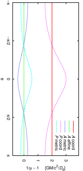
For $D_{\smash{\text{s}}}\to\infty$ this cancels the $m/2$ term in Eq. (31), which produced magnifications less than unity for large $\theta$. The same is true for the case with finite $D_{\smash{\text{s}}}$ in Eqs. (61–63). See Fig. 6 for a graphical illustration.

C.2 Metric distance

Alternatively, we could for the comparison of lensed and unlensed situation keep the metric distance $L$ constant, which we define as measured with a rigid ruler being at rest in the $(t,\mn@boldsymbol{r})$ coordinates of the weak-field metric. This can be integrated easily for a point mass at the standard position of Eq. (18):

$$L =\int\sqrt{-\text{d}s^{2}}\bigr{|}_{\text{d}t=0}=\int_{0}^{D_{\smash{\text{s}}}}\text{d}z\,\left[1-\frac{\Psi(x=0,z)}{c^{2}}\right]$$ (114)

$$=D_{\smash{\text{s}}}+\frac{GM}{c^{2}}\int_{0}^{D_{\smash{\text{s}}}}\text{d}z\,\frac{1}{\sqrt{\smash[b]{x_{0}^{2}+(z-z_{0})^{2}}}}$$ (115)

$$=D_{\smash{\text{s}}}+\frac{GM}{c^{2}}\ln\frac{D_{\smash{\text{s}}}-D_{\smash{\text{d}}}\cos\theta+D_{\smash{\text{ds}}}(\theta)}{D_{\smash{\text{d}}}(1-\cos\theta)}$$ (116)

$$=D_{\smash{\text{s}}}+\frac{GM}{c^{2}}\ln\frac{D_{\smash{\text{ds}}}(\theta)+D_{\smash{\text{d}}}+D_{\smash{\text{s}}}}{D_{\smash{\text{ds}}}(\theta)+D_{\smash{\text{d}}}-D_{\smash{\text{s}}}}\hskip 5.0pt\text{.}$$ (117)

To correct the magnifications to be valid for fixed $L$, they have to be multiplied with $(L/D_{\smash{\text{s}}})^{2}$ in the same way as above. Results are shown in Fig. 6.

Appendix D Lensing by a spherical shell

A very instructive example is that of a thin spherical shell acting as a lens, with the observer in the centre of the shell and the source sphere at infinity. Due to the symmetry, radial light rays are not deflected, so that we do not expect magnification caused by deflection. In the formalism of this paper, see Eq. (41), the constant surface mass density leads to a constant potential and no deflection or magnification. In the formalism of the focusing theorem, on the other hand, where the affine distance is kept constant to compare the lensed and unlensed situation, we still have focusing without deflection. One might think that the case of infinite focusing would allow a discussion without the arbitrariness of distance definitions, because different distances can only rescale the focusing.

In order to discuss this case, we have to leave the weak-field approximation and use the full metric for a shell with total mass $M$, $R_{M}=GM/c^{2}$ and radius $r_{0}$ in Schwarzschild coordinates:

$$\text{d}s^{2} =\begin{cases}\displaystyle\left(1-\frac{2R_{M}}{r_{0}}\right)\,\text{d}t^{2}-\text{d}r^{2}-r^{2}\,\text{d}\Omega^{2}&\text{for $r<r_{0}$}\\ \displaystyle\left(1-\frac{2R_{M}}{r}\right)\,\text{d}t^{2}-\left(1-\frac{2R_{M}}{r}\right)^{-1}\,\text{d}r^{2}-r^{2}\,\text{d}\Omega^{2}&\text{for $r>r_{0}$}\end{cases}$$ (118)

We are especially interested in the limiting case of undistorted global geometry of the Universe, therefore we consider very small $r_{0}$ and $M$, but keep $R_{M}/r_{0}$ constant. Using Eq. (6) it can be shown that in the weak field limit we have

$$\sigma =\frac{R_{M}}{r_{0}}\hskip 5.0pt\text{,}$$ (119)

which we extend as a definition of $\sigma$ for strong fields. In the limit of small $R_{M}$, the metric is distorted only in a small region around the observer. The radial metric distance then corresponds to $r$. The affine distance can be calculated with methods similar to those described in Appdendix C.1, which results in

$$\Lambda =\frac{r}{\sqrt{1-2\sigma}}\approx(1+\sigma)\,r\hskip 5.0pt\text{.}$$ (120)

The magnification defined for an unchanged affine distance scales with

$$\mu_{\Lambda} =\left(\frac{\Lambda}{r}\right)^{2}=\frac{1}{1-2\sigma}\hskip 5.0pt\text{,}$$ (121)

which obeys the focusing theorem $\mu_{\Lambda}>1$.

The critical case $\sigma=1/2$ corresponds to a lens which forms a black hole, which is clearly beyond the weak-field approximation. Even in more moderate cases, we see that the “focusing” is purely a result of the local measurement of the affine distance, which is affected by the metric distortions.

References

- Avni & Shulami (1988) Avni Y., Shulami I., 1988, ApJ, 332, 113
- Einstein (1936) Einstein A., 1936, Science, 84, 506
- Ellis (2007) Ellis G. F. R., 2007, General Relativity and Gravitation, 39, 1047
- Etherington (1933) Etherington I. M. H., 1933, Phil. Mag., 15, 761
- Etherington (2007) Etherington I. M. H., 2007, General Relativity and Gravitation, 39, 1055
- Jaroszyński & Paczyński (1996) Jaroszyński M., Paczyński B., 1996, Acta Astronomica, 46, 361
- Perlick (2004) Perlick V., 2004, Living Reviews in Relativity, 7, 9
- Refsdal (1964) Refsdal S., 1964, MNRAS, 128, 295
- Schneider (1984) Schneider P., 1984, A&A, 140, 119
- Schneider et al. (1992) Schneider P., Ehlers J., Falco E. E., 1992, Gravitational Lenses. Springer
- Virbhadra & Ellis (2000) Virbhadra K. S., Ellis G. F. R., 2000, Phys. Rev. D, 62, 084003
- Weinberg (1976) Weinberg S., 1976, ApJ, 208, L1