INSTITUT NATIONAL DE RECHERCHE EN INFORMATIQUE ET EN AUTOMATIQUE

Modular Compilation of a Synchronous Language
Daniel Gaffé — Annie Ressouche — Valérie Roy N° 6424

Abstract: Synchronous languages rely on formal methods to facilitate the developement of applications in an efficient and reusable way. In fact, formal methods have been advocated as a means of increasing the reliability of systems, especially those which are safety or business critical. It is even more difficult to develop automatic specification and verification tools due to limitations such as state explosion, undecidability, etc… In this work, we design a new specification model based on a reactive synchronous approach. We benefit from a formal framework well suited to perform compilation and formal validation of systems. In practice, we design and implement a special purpose language (le) with two semantic: its behavioral semantic helps us to define a program by the set of its behaviors and avoid ambiguity in programs interpretation; its equational semantic allows the compilation of programs into software and hardware targets (C code, Vhdl code, Fpga synthesis, Model checker input format). Our approach is relevant with respect to the two main requirements of critical realistic applications: modular compilation allows us to deal with large systems, while model-based approach provides us with formal validation. There is still a lack of efficient and modular compilation means for synchronous languages. Despite of relevant attempts to optimize generated code, no approach considers modular compilation. This report tackles this problem by introducing a compilation technique which relies on the equational semantic to ensure modularity completed by a new algorithm to check causality cycles in the whole program without checking again the causalty of sub programs.

Key-words: synchronous language, modular compilation, behavioral semantic, equational constructive semantic, modularity, separate compilation.

Compilation modulaire d’un langage synchrone

Résumé : Dans ce rapport, nous étudions le développement de systèmes critiques. Les méthodes formelles se sont avérées un moyen efficace pour augmenter la fiabilité de tels systèmes, en particulier ceux qui requièrent une certaine sécurité de fonctionnement. Neanmoins, le développement d’outils automatiques de spécification et de vérification est limité entre autre par la taille des modèles formels des systèmes ou par des problèmes d’indécidabilité. Dans ce travail, nous définissons un langage réactif synchrone (le) dédié à la spécification de systèmes critiques. Ce faisant, nous bénéficions d’un cadre formel sur lequel nous nous appuyons pour compiler séparement et valider les applications. Plus précisement, nous définissons deux sémantiques pour notre langage: une sémantique comportementale qui associe à un programme l’ensemble de ses comportements et évite ainsi toute ambiguité dans l’interpretation des programmes. Nous définissons aussi une sémantique équationnelle dirigeant la compilation de programmes vers différentes cibles (code c, code vhdl, synthétiseurs fpga, observateurs), permettant ainsi de traiter des applications logicielles et matérielles et aussi de les valider. Notre approche est pertinente vis à vis des deux principales exigences de réelles applications critiques: la compilation modulaire permet de traiter des applications conséquentes et l’approche formelle permet la validation. On peut constater que le domaine des langages synchrones manque encore de méthodes pour compiler les programmes de façon efficace et modulaire. Bien sur, certaines approches optimisent les codes produits d’un facteur important, mais aucune d’entre elles n’envisagent une compilation modulaire.

Mots-clés : langage synchrone, compilation modulaire , sémantique comportementale sémantique constructive equationnelle, modularité, compilation séparée.

1 Introduction

We address the design of safety-critical control-dominated systems. By design we mean all the work that must be done from the initial specification of a system to the embedding of the validated software into its target site. The way control-dominated systems work is reactive in the sense of D. Harel and A. Pnueli definition[11]: they react to external stimuli at a speed defined and controlled by the system’s environment. The evolution of a reactive system is a sequence of reactions raised by the environment. A control-dominated application can then be naturally decomposed into a set of communicating reactive sub-systems each dealing with some specific part of the global behavior, combined together to achieve the global goal.

It is now stated that general purpose programming languages are not suited to design reactive systems: they are clearly inefficient to deal with the inherent complexity of such systems. From now on, the right manner to proceed is to design languages dedicated to reactive systems. To this aim, synchronous languages such as Esterel[3] and SyncCharts [1], dedicated to specify event-driven applications; Lustre and Signal[9], data flow languages well suited to describe signal processing applications like, have been designed. They are model-based languages to allow formal verification of the system behavior and they agree on three main features:

1. Concurrency: they support functional concurrency and they rely on notations that express concurrency in a user-friendly manner. le adopts an imperative Esterel-like style to express parallelism. However, the semantic of concurrency is the same for all synchronous languages and simultaneity of events is primitive.

2. Simplicity: the language formal models are simple (usually mealy machines or netlists) and thus formal reasoning is made tractable. In particular, the semantic for parallel composition is clean.

3. Synchrony: they support a very simple execution model. First, memory is initialized and then, for each input event set, outputs are computed and then memory is updated. Moreover, all mentioned actions are assumed to take finite memory and time.

Synchronous languages rely on the synchronous hypothesis which assumes a discrete logic time scale, made of instants corresponding to reactions of the system. All the events concerned by a reaction are simultaneous: input events as well as triggered output events. As a consequence, a reaction is instantaneous (we consider that a reaction takes no time), there are no concurrent partial reactions, and determinism is thus ensured.

There are numerous advantages to the synchronous approach. The main one is that temporal semantic is simplified, thanks to the afore mentioned logical time. This leads to clear temporal constructs and easier time reasoning. Another key advantage is the reduction of state-space explosion, thanks again to discrete logical time: systems evolve in a sequence of discrete steps, and nothing occurs between two successive steps. A first consequence is that program debugging, testing, and validating is easier. In particular, formal verification of synchronous programs is possible with techniques like model checking. Another consequence is that synchronous language compilers are able to generate automatically embeddable code, with performances that can be measured precisely.

Although synchronous languages have begun to face the state explosion problem, there is still a need for further research on their efficient and modular compilation. The initial compilers translated the program into an extended finite state machine. The drawback of this approach is the potential state explosion problem. Polynomial compilation was first achieved by a translation to equation systems that symbolically encode the automata. This approach is successfully used for hardware synthesis and is the core of commercial tools [15] but the generated software may be very slow. Then several approaches translate the program into event graphs [16] or concurrent data flow graphs [7, 13] to generate efficient C code. All these methods have been used to optimize the compilation times as well as the size and the execution of the generated code.

However none of these approaches consider a modular compilation. Some attempts allow a distributed compilation of programs [16, 7] but no compilation mechanism relies on a modular semantic of programs. Of course there is a fundamental contradiction in relying on a formal semantic to compile reactive systems because a perfect semantic would combine three important properties: responsiveness, modularity and causality. Responsiveness means that we can deal with a logical time and we can consider that output events occur in the same reaction as the input events causing them. It is one of the foundations of the synchronous hypothesis. Causality means that for each event generated in a reaction, there is a causal chain of events leading to this generation; no causality loop may occur. A semantic is modular when “environment to component” and “component to component” communication are treated symmetrically. In particular, the semantic of the composition of two reactive systems can be deduced from the respective semantic of each sub-part. Another aspect of modularity is the coherent view each subsystem has of what is going on. When an event is present, it is broadcasted all around the system and is immediately available for every part which listens to it. Unfortunately, there exists a theorem (“the RMC barrier theorem”) [12] that states that these three properties cannot hold together in a semantic. Synchronous semantic are responsive and modular. But causality remains a problem in these semantic and modular compilation must be completed by a global causality checking.

In this paper we introduce a reactive synchronous language, we define its behavioral semantic that gives a meaning to programs and an equational semantic allowing first, a modular compilation and, second, a separate verification of properties. Similarly to other synchronous semantic, we must check that programs have no potential causality loop. As already mentioned, causality can only be checked globally since a bad causality may be created when performing the parallel composition of two causal sub programs. We compile le programs into equation systems and the program is causal if its compilation is cycle free. The major contribution of our approach relies on the introduction of a new sorting algorithm that allows us to start from already compiled and checked subprograms to compile and check the overall program without sorting again all the equations.

2 LE Language

le language belongs to the family of reactive synchronous languages. It is a discrete control dominated language. We first describe its syntax (the overall grammar is detailed in appendix A).

The le language unit are named modules. The language’s operators and constructions are chosen to fit the description of reactive applications as a set of concurrent communicating sub-systems. Communication takes place between modules or between a module and its environment. Sub-system communicates via events.

The module interface declares the set of input events it reacts to and the set of output events it emits. For instance, the following piece of code shows the declarative part of a Control module used in the example in section 6.

module Control:
Input:forward, backward, upward,  downward, StartCycle;
Output:MoveFor, MoveBack, MoveDown, SuckUp, EndCycle ;

2.1 LE Statements

The module body is expressed using a set of control operators. They are the cornerstone of the language because they operate over event’s status. Some operators terminate instantaneously, some other takes at least one instant. We mainly distinguish two kinds of operators: usual programming language operators and operators devoted to deal with logical time.

2.1.1 Non Temporal Statements

le language offers two basic instructions:

• The nothing instruction does "nothing" and terminates instantaneously.

• The event emission instruction (emit speed) sets to present the status of the emitted signal.

Moreover, some operators help us to built composite instructions:

• The present-then-else instruction (present S { P1} else { P2}) is a usual conditional statement except that boolean combinations of signals status are used as conditions.

• In the sequence instruction ($P_{1}\gg P_{2}$) the first sub-instruction $P_{1}$ is executed. Then, if $P_{1}$ terminates instantaneously, the sequence executes immediately its second instruction $P_{2}$ and stops whenever $P_{2}$ stops. If $P_{1}$ stops, the sequence stops. The sequence terminates at the same instant as its second sub-instruction $P_{2}$ terminates. If the two sub-instructions are instantaneous, the sequence terminates instantaneously.

• The parallel instruction($P_{1}\|P_{2}$) begins the execution of its two sub-instructions at the same instant. It terminates when both sub-instructions terminate. When the two sub-instructions are instantaneous, the parallel is instantaneous. Notice that the parallel instruction agrees with the synchronous hypothesis and allows the simultaneity of trigger signals causing $P_{1}$ or $P_{2}$.

• A strong or weak preemption instruction over a signal $S$ can surround an instruction $P$ as in: $abort\ P\ when\ S$. While the signal status evaluates to “absent”, instruction $P$ continues its execution. The instant the event evaluates to “present”, the instruction is forced to terminate. When the instruction is preempted, the weak preemption let the instruction ends its current execution while the strong one does not. If the instruction terminates normally without been preempted, the preemption instruction also terminates and the program execution continues.

• A Loop instruction ($loop\ \{P\}$) surrounds an instruction $P$. Instruction $P$ is automatically restarted the same instant it terminates. The body of a loop cannot be instantaneous since it will start again the execution of its body within the same instant.

• Local signals instruction ($local\ S\ \{P\}$) is used to encapsulate communication channels between two sub systems. The scope of $S$ is restricted to $P$. As a consequence, each local signal tested within the body of the local instruction must be emitted from the body.

• A module call instruction($Run$) is used to run an external module inside another module. Recursive calls of module are not allowed. Running a module does not terminate instantaneously. In the declarative part of the module, you can specify the paths where the already compiled code of the called modules are:

  Run: "./TEST/control/" : Temporisation;
  Run: "./TEST/control/" : NormalCycle;
  

2.1.2 Temporal Statements

There are two temporal operators in le .

• The pause instruction stops for exactly one reaction.

• The waiting instruction (wait S) waits the presence of a signal. The first time the execution of the program reaches a wait instruction, the execution stops (whatever the signal status is). At the beginning of the following instant, if the signal status is tested “present” the instruction terminates and the program continues its execution, otherwise it stays stopped.

2.1.3 Automata Specification

Because it remains difficult to design an automaton-like behavior using the previously mentioned operators, our language offers an automaton description as a native construction. An automata is a set of states and labeled transitions between states. Some transitions are initial and start the automata run while terminal states indicate that the automaton computation is over. The label of transitions have two fields: a trigger which is a boolean combination of signal status and an output which is the list of signals emitted when the transition is taken (i.e when the trigger part is true). le automata are Mealy machines and they have a set of input signals to define transition triggers and a set of output signals that can be emitted when a transition is raised. In le , the body of a module is either an instruction or an automaton. It is not allowed to build new instructions by combining instructions and automata. For instance, the only way to put in parallel an automaton and the emission of a signal is to call the module the body of which is the automata through a run operation. Practically, we offer a syntactic means to describe an automaton (see appendix A for a detailed syntax). Moreover, our graphical tool (galaxy) helps users edit automata and generate the le code.

3 LE Behavioral Semantic

le behavioral semantic is useful to give a meaning to each program and thus to define its behavior without ambiguity. To define the behavioral semantic of le, we first introduce a logical context to represent events, then we define the le process calculus in order to describe the behavioral semantic rules.

3.1 Mathematical Context

Similarly to others synchronous reactive languages, le handles broadcasted signals as communicating means. A program reacts to input events by producing output events. An event is a signal carrying some information related to its status. The set of signal status $\xi$ ($\xi$ = $\{\bot,0,1,\top\}$) is intented to record the status of a signal at a given instant. Let $S$ be a signal, $S^{x}$ denotes its instant current status. More precisely, $S^{1}$ means that $S$ is present, $S^{0}$ means that $S$ is absent, $S^{\bot}$ means that $S$ is neither present nor absent and finally $S^{\top}$ corresponds to an event whose status cannot be induced because it has two incompatible status in two different sub parts of the program. For instance, if $S$ is both absent and present, then it turns out to have $\top$ status and thus an error occurs. Indeed. the set $\xi$ is a complete lattice with the $\leq$ order:

$$\begin{array}[]{c c c}&\top&\\ \nearrow&&\nwarrow\\ 0&\uparrow&\quad 1\\ \nwarrow&&\nearrow\\ &\bot&\\ \end{array}$$

Composition Laws for $\xi$

We define 3 internal composition laws in $\xi$: $\>\boxplus\>$, $\>\boxdot\>$and $\neg$ (to extend the usual operations defined for classical boolean set IB), as follows:

The $\>\boxplus\>$ law is a binary operation whose result is the upper bound of its operands:

$\>\boxplus\>$	$1$	$0$	$\top$	$\bot$
$1$	$1$	$\top$	$\top$	$1$
$0$	$\top$	$0$	$\top$	$0$
$\top$	$\top$	$\top$	$\top$	$\top$
$\bot$	$1$	$0$	$\top$	$\bot$

Particularly:

• $\bot$ $\>\boxplus\>$$\bot=\bot$;

• $1$$\>\boxplus\>$$0=0$$\>\boxplus\>$$1=\top$;

• $\top$ is an absorbing element;

The $\>\boxdot\>$law is a binary operation whose result is the lower bound of its operands:

$\>\boxdot\>$	$1$	$0$	$\top$	$\bot$
$1$	$1$	$\bot$	$1$	$\bot$
$0$	$\bot$	$0$	$0$	$\bot$
$\top$	$1$	$0$	$\top$	$\bot$
$\bot$	$\bot$	$\bot$	$\bot$	$\bot$

Particularly:

• $\top\>\boxdot\>\top=\top$;

• $1\>\boxdot\>0=0\>\boxdot\>1=\bot$;

• $\bot$ is an absorbing element;

Finally, the $\neg$ law is an inverse law in $\xi$:

$x$	$\neg\ x$
$1$	$0$
$0$	$1$
$\top$	$\bot$
$\bot$	$\top$

The set $\xi$ with these 3 operations verifies the axioms of Boolean Algebra: commutative and associative axioms for $\>\boxplus\>$and $\>\boxdot\>$, distributive axioms both for $\>\boxdot\>$over $\>\boxplus\>$and for $\>\boxplus\>$over $\>\boxdot\>$, neutral elements for $\>\boxplus\>$and $\>\boxdot\>$and complementarity.

Commutativity:	$x$ $\>\boxplus\>$$y=y$ $\>\boxplus\>$$x$	$x\>\boxdot\>y=y\>\boxdot\>x$	(1)
Associativity:	$(x$ $\>\boxplus\>$$y)$ $\>\boxplus\>$$x=x$ $\>\boxplus\>$$(y$$\>\boxplus\>$$z)$	$(x\>\boxdot\>y)\>\boxdot\>x=x\>\boxdot\>t(y\>\boxdot\>z)$	(2)
Distributivity:	$x\>\boxdot\>(y$$\>\boxplus\>$$z)=(x\>\boxdot\>y)$ $\>\boxplus\>$$(x\>\boxdot\>z)$	$x$$\>\boxplus\>$$(y\>\boxdot\>z)=(x$$\>\boxplus\>$$y)\>\boxdot\>(x$$\>\boxplus\>$$z)$	(3)
Neutral elements:	$x$$\>\boxplus\>$$\bot=x$	$x\>\boxdot\>\top=x$	(4)
Complementarity:	$x$$\>\boxplus\>$$\neg\ x=\top$	$x\>\boxdot\>\neg\ x=\bot$	(5)

Axioms (1) and (4) are obvious looking at the previous tables that define the $\>\boxplus\>$and $\>\boxdot\>$laws. Axioms (2) and (4) are also obviously true but their proofs necessitate to compute the appropriate tables. Finally, axiom (5) results from the following table:

$x$	$x$ $\>\boxplus\>$$\neg\ x$	$x\>\boxdot\>\neg\ x$
$1$	$1$ $\>\boxplus\>$$0=\top$	$1\>\boxdot\>0=\bot$
$0$	$0$ $\>\boxplus\>$$1=\top$	$0\>\boxdot\>1=\bot$
$\top$	$\top$ $\>\boxplus\>$$\bot=\top$	$\top\>\boxdot\>\bot=\bot$
$\bot$	$\bot$ $\>\boxplus\>$$\top=\top$	$\bot\>\boxdot\>\top=\bot$

As a consequence, $\xi$ is a Boolean algebra and the following theorems are valid:

Identity law:	$x$ $\>\boxplus\>$$x=x$	$x\>\boxdot\>x=x$
Redundancy law:	$x$ $\>\boxplus\>$$(x\>\boxdot\>y)=x$	$x\>\boxdot\>(x$$\>\boxplus\>$$y)=x$
Morgan law:	$\neg\ (x$ $\>\boxplus\>$$y)=\neg\ x\>\boxdot\>\neg\ y$	$\neg\ (x\>\boxdot\>y)=\neg\ x$$\>\boxplus\>$$\neg\ y$
Neutral element:	$x$ $\>\boxplus\>$$\top=\top$	$x\>\boxdot\>\bot=\bot$

In such a setting, $xor$, $nor$, $nand$, $\Leftrightarrow$, $\Rightarrow$ are defined:

$x\ xor\ y$	=	$x\>\boxdot\>\neg\ y$$\>\boxplus\>$$y\>\boxdot\>\neg\ x$
$x\ nor\ y$	=	$\neg\ x\>\boxdot\>\neg\ y$
$x\ nand\ y$	=	$\neg\ x$$\>\boxplus\>$$\neg\ y$
$x\Leftrightarrow y$	=	$(\neg\ x\>\boxdot\>\neg\ y)$ $\>\boxplus\>$$(x\>\boxdot\>y)$
$x\Rightarrow y$	=	$\neg x$ $\>\boxplus\>$$y$

Hence, we can apply these classical results concerning Boolean algebras to solve equation systems whose variables belong to $\xi$. For instance, the equational semantic detailed in section 4 relies on boolean algebra properties to compute signal status as solution of status equations.

Moreover, since $\xi$ is a lattice, the $\>\boxplus\>$and $\>\boxdot\>$operations are monotonic: let $x$, $y$ and $z$ be elements of $\xi$, ($x\leq y)\Rightarrow(x\>\boxplus\>z\leq y\>\boxplus\>z$) and ($x\leq y)\Rightarrow(x\>\boxdot\>z\leq y\>\boxdot\>z)$.

Condition Law

We introduce a condition law ($\blacktriangleleft$) in $\xi$ to drive a signal status with a boolean condition:

$\xi\ \times\ \leavevmode\mbox{I}\!\mbox{B}$	$\longrightarrow$	$\xi$
$(x,c)$	$\longmapsto$	$x\blacktriangleleft c$

This law is defined by the following table:

$x$	$c$	$x\blacktriangleleft c$
$1$	$0$	$\bot$
$0$	$0$	$\bot$
$\top$	$0$	$\bot$
$\bot$	$0$	$\bot$
$1$	$1$	$1$
$0$	$1$	$0$
$\top$	$1$	$\top$
$\bot$	$1$	$\bot$

This condition law allows us to change the status of an event according to a boolean condition. It will be useful to define both le behavioral and equational semantic since the status of signals depend of the termination of the instructions that compose a module. Intuitively, a signal keeps its status if the condition is true, otherwise its status is set to $\bot$.

Relation between $\xi$ and $\leavevmode\mbox{I}\!\mbox{B}^{2}$

$\xi$ is bijective to $\leavevmode\mbox{I}\!\mbox{B}\times\leavevmode\mbox{I}\!\mbox{B}$. We define the following encoding:

signal status	encoding
$1$	$11$
$0$	$10$
$\top$	$01$
$\bot$	$00$

Hence, a signal status is encoded by 2 boolean variables. The first boolean variable of the status of a signal ($S$) is called its definition ($S_{def}$), while the second one is called its value ($S_{val}$). According to the encoding law, when $S_{def}=0$ the signal $S$ has either $\top$ or $\bot$ value for status and it is not defined as present or absent. On the opposite, when $S_{def}=1$, the signal is either present or absent. It is why we choose to denote the first boolean projection of a signal status by $S_{def}$.

IB is the classical boolean set with 3 operators and (denoted .), or (denoted +) and not (denoted $\overline{x}$, for boolean $x$). According to the previous encoding of $\xi$ into $\leavevmode\mbox{I}\!\mbox{B}\times\leavevmode\mbox{I}\!\mbox{B}$ and after algebraic simplification, we have the following equalities related to $\>\boxplus\>$, $\>\boxdot\>$and $\neg$ operators. Let $X$ and $Y$ be 2 elements of $\xi$:

($X$ $\>\boxplus\>$$Y)_{def}$	=	$X_{def}.\overline{Y_{def}}.\overline{Y_{val}}+Y_{def}.\overline{X_{def}}.\overline{X_{val}}+(X_{def}.Y_{def}).\overline{(X_{val}\oplus Y_{val})}$
($X$ $\>\boxplus\>$$Y)_{val}$	=	$X_{val}+Y_{val}$
($X\>\boxdot\>Y)_{def}$	=	$X_{def}.\overline{Y_{def}}.Y_{val}+Y_{def}.\overline{X_{def}}.X_{val}+(X_{def}.Y_{def}).\overline{(X_{val}\oplus Y_{val})}$
($X\>\boxdot\>Y)_{val}$	=	$X_{val}.Y_{val}$
($\neg\ X)_{def}$	=	$X_{def}$
($\neg\ X)_{val}$	=	$\overline{X_{val}}$
$(X\blacktriangleleft c)_{def}$	=	$X_{def}.c$
$(X\blacktriangleleft c)_{val}$	=	$X_{val}.c$

where $\oplus$ is the exclusive or operator of classical boolean set. The proof of the last equality is detailed in appendix D.

On the opposite side, we can expand each boolean element into a status member, 0 correspond to 0, and 1 to 1. More precisely let $x$ be an element of IB and $\xi(x)$ its corresponding status, then $\xi(x)_{def}=1$ and $\xi(x)_{val}=x$.

Notion of Environment

An environment is a finite set of events. Environments are useful to record the current status of signals in a reaction. Thus a signal has a unique status in an environment: if $S^{x}$ and $s^{y}$ belongs to the same environment, then $x=y$.

We extend the operation defined in $\xi$ to environments. Let $E$ and $E^{\prime}$ be 2 environments:

$E$ $\>\boxplus\>$$E^{\prime}$	=	$\{S^{z}|\exists S^{x}\in E,S^{y}\in E^{\prime},z=x$$\>\boxplus\>$$y\}$
$E\>\boxdot\>E^{\prime}$	=	$\{S^{z}|\exists S^{x}\in E,S^{y}\in E^{\prime},z=x\>\boxdot\>y\}$
$\neg E$	=	$\{S^{\neg\ x}|\exists S^{x}\in E\}$
$E\ \blacktriangleleft\ c$	=	$\{S\ \blacktriangleleft\ c\ |\ S\in E\}$

We define a relation ($\preceq$) on environments as follows:

$$E\preceq E^{\prime}\ {\rm iff}\ \forall S^{x}\in E,\exists S^{y}\in E^{\prime}|S^{x}\leq S^{y}$$

Thus $E\preceq E^{\prime}$ means that $E$ is included in $E^{\prime}$ and that each element of $E$ is less than an element of $E^{\prime}$ according to the lattice order of $\xi$. As a consequence, the $\preceq$ relation is a total order on environments and $\>\boxplus\>$and $\>\boxdot\>$operations are monotonic according to $\preceq$.

Finally, we will denote $E^{\top}$, the environment where all events have $\top$ status.

3.2 LE Behavioral Semantic

In order to describe the behavioral semantic of le , we first introduce a process algebra associated with the language. Then we can define the semantic with a set of rewriting rules that determines a program execution. The semantic formalize a reaction of a program $P$ according to an event input set. $P\begin{array}[]{c}E^{\prime}\\ \boldsymbol{\longmapsto}\\ E\end{array}P^{\prime}$ has the usual meaning: $E$ and $E^{\prime}$ are respectively input and output environments; program $P$ reacts to $E$, reaches a new state represented by $P^{\prime}$ and the output environment is $E^{\prime}$. To compute such a reaction we rely on the behavioral semantic of le . This semantic supports a rule-based specification to describe the behavior of each operator of le process algebra associated with le language. A rule has the form: $p\xrightarrow[E]{E^{\prime},TERM}p^{\prime}$ where $p$ and $p^{\prime}$ are elements of le process algebra. $E$ is an environment that specifies the status of the signals declared in the scope of $p$, $E^{\prime}$ is the output environment and $TERM$ is a boolean flag true when $p$ terminates. This notion of termination differs from the one used in Esterel language successive behavioral semantic. It means from the current reaction, $p$ is able to terminate and this information will be sustained until the real termination occurs.

Let $P$ be a le program and $p$ its corresponding process algebra term. Given an input event set $E$, a reaction is computed as follows:

$$P\begin{array}[]{c}E^{\prime}\\ \boldsymbol{\longmapsto}\\ E\end{array}P^{\prime}\hskip 14.22636pt{\rm iff}\hskip 14.22636ptp\xrightarrow[E]{E^{\prime},\ TERM}p^{\prime}$$

LE Process Calculus (PLE)

The ple process algebra associated to le language is defined as follows:

• nothing;

• halt;

• !s (emit s);

• wait s;

• iwait s (wait immediate s);

• s ? $p$ : $q$ (present s {$p$} else {$q$});

• $p\|q$;

• $p\gg q$;

• $p\uparrow_{\texttt{\small{s}}}$ (abort {$p$} when s);

• $p*$ (loop {p});

• $p\backslash\texttt{\small{s}}$ (local s {$p$});

• ${\cal A}({\cal M},{\cal T},{\cal C}ond,M_{f},{\cal O},\lambda)$. Automata ${\cal A}$ is a structure made of 6 components:

  1. a finite set of macro states (${\cal M}$). Each macro state $M$ may be is itself composed of a sub term $p$ (denoted $M[p]$);

  2. a finite set of conditions (${\cal C}ond$);

  3. a finite set of transitions (${\cal T}$). A transition is a 3-uple $<M,c,M^{\prime}>$ where $c\in{\cal C}ond$ is a boolean condition raising the transition from macro state $M$ to macro state $M^{\prime}$. We will denote $M\rightarrow M^{\prime}$ for short in the rest of the report and $c_{M\rightarrow M^{\prime}}$ will denote the condition associatesd with the transition. . ${\cal T}$ is also composed of initial transitions of the form: ${\rightarrow M^{\prime}}$. They are useful to start the automata run. When condition $c$ is true, the macro state $M^{\prime}$ is reached;

  4. a final macro state $M_{f}$;

  5. a finite set of output signals (${\cal O}$) paired with an output function $\lambda$ that links macro states and output signals: $\lambda:{\cal T}\longrightarrow{\cal P}({\cal O})$, defined as follows: $\lambda({M\rightarrow M^{\prime}})=o\subseteq{\cal O}$ is the set of output signals emitted when the trigger condition $c_{M\rightarrow M^{\prime}}$ is true.

Each instruction of le has a natural translation as an operator of the process algebra. As a consequence, we associate a term of the process algebra with the body of each program while the interface part allows to build the global environment useful to define the program reaction as a rewriting of the behavioral semantic. Notice that the operator iwait s does not correspond to any instruction of the language, it is introduced to express the semantic of the wait statement. It is a means to express that the behavior of a term takes at least one instant. It is the case of wait s that skip an instant before reacting to the presence of s.

More precisely, we introduce a mapping: $\Gamma$ : le $\rightarrow$ ple , which associates a ple term with each le program. $\Gamma$ is defined according to the syntax of the le language.

Let $P$ be a le program, $\Gamma(P)$ is structurally defined on the body of $P$.

• $\Gamma({\rm nothing})=\texttt{\small{nothing}}$;

• $\Gamma({\rm halt})=\texttt{\small{halt}}$;

• $\Gamma({\rm emit}\ \texttt{\small{s}})=!\texttt{\small{s}}$;

• $\Gamma({\rm wait}\ \texttt{\small{s}})=\texttt{\small{wait s}}$;

• $\Gamma({\rm present}\texttt{\small{s}}P_{1}\ {\rm else}\ P_{2})=\texttt{\small{s}}?\Gamma(P_{1}):\Gamma(P_{2})$;

• $\Gamma(P_{1}\|P_{2})=\Gamma(P_{1})\|\Gamma(P_{2})$;

• $\Gamma(P_{1}\gg P_{2})=\Gamma(P_{1})\gg\Gamma(P_{2})$;

• $\Gamma({\rm abort}\ P_{1}\ {\rm when}\ \texttt{\small{s}})=\Gamma(P_{1})\uparrow_{\texttt{\small{s}}}$;

• $\Gamma({\rm loop}\ \{P_{1}\})=\Gamma(P_{1})*$;

• $\Gamma({\rm local}\ \texttt{\small{s}}\{P_{1}\})=\Gamma(P_{1})\backslash\texttt{\small{s}}$;

• $\Gamma({\rm run}\ P_{1})=$ wait tick $\gg\Gamma(P_{1})$ where tick is a “clock” signal present in each reaction;

• $\Gamma({\cal A}({\cal M},{\cal T},{\cal C}ond,M_{f},{\cal O},\lambda)$ = ${\cal A}({\cal M},{\cal T},{\cal C}ond,M_{f},{\cal O},\lambda)$.

Behavioral Semantic Rules

The basic operators of le process algebra have the following rewriting rules. Both nothing and halt have no influence on the current environment, but the former is always ready to leave and the latter never. The emit operator is ready to leave and the signal emitted is set present in the environment .

$$\begin{array}[]{l l l r}\texttt{\small{nothing}}&\xrightarrow[E]{E,\ 1}&\texttt{\small{nothing}}&\qquad\qquad(nothing)\\ \texttt{\small{halt}}&\xrightarrow[E]{E,\ 0}&\texttt{\small{nothing}}&\qquad\qquad(halt)\\ !\texttt{\small{s}}&\xrightarrow[E]{E[\texttt{\small{s}}\leftarrow 1],\ 1}&\texttt{\small{nothing}}&\qquad\qquad(emit)\\ \end{array}$$

Wait

The semantic of wait is to wait at least one instant. Thus, to express its behavior, we introduce the iwait operator. Then, wait s is not ready to leave, and rewrites into iwait s. This rewriting behaves like wait s except that it reacts instantaneously to the signal presence.

$$\texttt{\small{wait s}}\xrightarrow[E]{E,\ 0}{\texttt{\small{iwait s}}}\qquad\qquad(wait)$$

$$\frac{\texttt{\small{s}}^{1}\in E}{\texttt{\small{iwait s}}\xrightarrow[E]{E,\ 1}\texttt{\small{nothing}}}\quad(iwait1)\qquad\frac{\texttt{\small{s}}^{1}\not\in E}{\texttt{\small{iwait s}}\xrightarrow[E]{E,\ 0}\texttt{\small{iwait s}}}\quad(iwait2)\qquad$$

Present

The semantic of $\texttt{\small{s}}\ ?\ p\ :\ q$ operator depends on the status of s in the initial environment $E$. If s is present (resp absent) in $E$, the operator behaves like $p$ (resp $q$) (rules $present1$ and $present2$). Otherwise, if s is undefined we cannot progress in the rewriting system (rule $present3$) and if the computation of s internal status results in $\top$, it is an error and this last is propagated (each event is set to error in the environment).

$$\frac{p\xrightarrow[E]{E_{p},\ TERM_{p}}p^{\prime},q\xrightarrow[E]{E_{q},\ TERM_{q}}q^{\prime},\texttt{\small{s}}^{1}\in E}{\texttt{\small{s}}\ ?\ p\ :\ q\xrightarrow[E]{E_{p},\ TERM_{p}}p^{\prime}}\quad(present1)\qquad$$

$$\frac{p\xrightarrow[E]{E_{p},\ TERM_{p}}p^{\prime},q\xrightarrow[E]{E_{q},\ TERM_{q}}q^{\prime},\texttt{\small{s}}^{0}\in E}{\texttt{\small{s}}\ ?\ p\ :\ q\xrightarrow[E]{E_{q},\ TERM_{q}}q^{\prime}}\quad(present2)\qquad$$

$$\frac{p\xrightarrow[E]{E_{p},\ TERM_{p}}p^{\prime},q\xrightarrow[E]{E_{q},\ TERM_{q}}q^{\prime},\texttt{\small{s}}^{\bot}\in E}{\texttt{\small{s}}\ ?\ p\ :\ q\xrightarrow[E]{E,\ 0}\texttt{\small{s}}\ ?\ p\ :\ q}\quad(present3)\qquad$$

$$\frac{p\xrightarrow[E]{E_{p},\ TERM_{p}}p^{\prime},q\xrightarrow[E]{E_{q},\ TERM_{q}}q^{\prime},\texttt{\small{s}}^{\top}\in E}{\texttt{\small{s}}\ ?\ p\ :\ q\xrightarrow[E]{E^{\top},\ 1}\texttt{\small{s}}\ ?\ p\ :\ q}\quad(present4)\qquad$$

Parallel

The parallel operator computes its two arguments according to the broadcast of signals between both sides and it terminates when both sides do.

$$\frac{p\xrightarrow[E]{E_{p},\ TERM_{p}}p^{\prime}\quad,\quad q\xrightarrow[E]{E_{q},\ TERM_{q}}q^{\prime}}{p\|q\xrightarrow[E]{E_{p}\>\boxplus\>E_{q},\>TERM_{p}.TERM_{q}}p^{\prime}\|q^{\prime}}\quad(parallel)\qquad$$

Sequence

The sequence operator has the usual behavior. While the first argument does not terninate we don’t begin the computation of the second argument (rule $sequence1$). When it terminates , we start the second argument (rule $sequence2$).

$$\frac{p\xrightarrow[E]{E_{p},\ 0}p^{\prime}}{p\gg q\xrightarrow[E]{E_{p},\ 0}p^{\prime}\gg q}\quad(sequence1)\qquad\frac{p\xrightarrow[E]{E_{p},\ 1}\ \texttt{\small{nothing}},q\xrightarrow[E_{p}]{E_{q},\ TERM_{q}}q^{\prime}}{p\gg q\xrightarrow[E]{E_{q},\ TERM_{q}}q^{\prime}}\quad(sequence2)\qquad$$

Abort

The behavior of the abort operator first derives the body of the statement. Thus, if the aborting signal is present is the input environment, then the statement rewrites in nothing and terminates (rule $abort1$). If it is not, the body of the statement is derived again (rules $abort2$ and $abort3$)

$$\frac{p\xrightarrow[E]{E_{p},TERM_{p}}p^{\prime},{\texttt{\small{s}}^{1}\in E}}{p\uparrow_{\texttt{\small{s}}}\xrightarrow[E]{E_{p},\ 1}\texttt{\small{nothing}}}\quad(abort1)\qquad$$

$$\frac{\ p\xrightarrow[E]{E_{p},1}\texttt{\small{nothing}},\texttt{\small{s}}^{1}\not\in E}{p{\uparrow}_{\texttt{\small{s}}}\xrightarrow[E]{E_{p},1}\texttt{\small{nothing}}}\quad(abort2)\qquad\frac{\ p\xrightarrow[E]{E_{p},0}p^{\prime},\texttt{\small{s}}^{1}\not\in E}{p{\uparrow}_{\texttt{\small{s}}}\xrightarrow[E]{E_{p},0}p^{\prime}{\uparrow}_{\texttt{\small{s}}}}\quad(abort3)\qquad$$

Loop

Loop operator never terminates and $p*$ behaves as $p\gg p*$.

$$\frac{p\xrightarrow[E]{E_{p},0}p^{\prime}}{p*\xrightarrow[E]{E_{p},\ 0}p^{\prime}\gg p*}\quad(loop)\qquad$$

Local

Local operator behaves as an encapsulation. Local signals are no longer visible in the surrounding environment.

$$\frac{p\xrightarrow[E\cup\texttt{\small{s}}^{\bot}]{E_{p},\ TERM_{p}}p^{\prime}}{p\backslash\texttt{\small{s}}\xrightarrow[E]{E_{p}-\{\texttt{\small{s}}\},TERM_{p}}p^{\prime}\backslash\texttt{\small{s}}}\quad(local)\qquad$$

Automata

Automata are deterministic (i.e $\forall M\in{\cal M},\ \exists!{M\rightarrow M^{\prime}}\in{\cal T}$ such that $c_{M\rightarrow M^{\prime}}=1$).

The semantic of automata terms relies on macro state semantic. A macro state does not terminate within a single reaction. Its duration is at least one instant. Thus, $M[p]$ waits an instant and then has the same behavior than p.

$$M[p]\xrightarrow[E]{E,\ 0}p$$

If the macro state is only a state without sub term $p$, then

$$M\xrightarrow[E]{E,\ 0}nothing$$

Now, we define the rewriting rules for automata ${\cal A}$. The evaluation of a condition $c\in{\cal C}ond$ depends on the current status of signals in the environment. To denote the current value of a condition we will use the following notation: $E\models c=b$

Axiom:

$$\frac{{\rightarrow M}\in{\cal T},E\models c_{\rightarrow M}=1}{{\cal A}\xrightarrow[E]{E[s\leftarrow 1|s\in\lambda({{\rightarrow M}})],\ 0}<{\cal A},M,M[p]>}\quad(automata0)\qquad$$

Rewriting rules for automata describe the behavior of a reaction as usual. Thus, we define rewriting rules on a 3-uple: $<{\cal A},M,p>$. The first element of the tuple is the automaton we consider, the second is the macro state we are in, and the third is the current evaluation of the sub term involved in this macro state.

$$\frac{p\xrightarrow[E]{E_{p},TERM}p^{\prime},\quad\forall M^{\prime}\ {\rm such\ that\ }{M\rightarrow M^{\prime}}\in{\cal T}\ E_{p}\models\ \sum c_{M\rightarrow M^{\prime}}\neq 1}{<{\cal A},M,p>\xrightarrow[E]{E_{p},\ 0}<{\cal A},M,p^{\prime}>}\quad(automata1)\qquad$$

$$\frac{\exists M^{\prime}\ {\rm such\ that}\ {M\rightarrow M^{\prime}}\in{\cal T}{\rm\ and\ }E\models c_{M\rightarrow M^{\prime}}=1}{<{\cal A},M,p>\xrightarrow[E]{E[s\leftarrow 1|s\in\lambda({{M\rightarrow M^{\prime}}})],\ 0}<{\cal A},M^{\prime},M^{\prime}[p]>}\quad(automata2)\qquad$$

$$\frac{p\xrightarrow[E]{E_{p},1}nothing}{<{\cal A},M_{f},p>\xrightarrow[E]{E_{p},\ 1}nothing}\quad(automata3)\qquad$$

Rule $automata0$ is the axion to start the evaluation of the automaton. Rule $automata1$ expresses the behavior of ${\cal A}$ automata when all the transition trigger conditions are false: in such a case, the sub term associated with the current macro state is derived (whatever the derivation is) and the automata does not terminate. On the opposite side, rule $automata2$ expresses the automata behavior when a transition condition becomes true. In such a case, the automata steps to the next macro state specified in the condition and the emitted signals associated with the transition are set to 1 in the environment. Finally, rule $automata3$ is applied when the evaluation of the term included in the final macro state is over; then the automata computation is terminated.

The behavioral semantic is a “macro” semantic that gives the meaning of a reaction for each term of the le process algebra. Nevertheless, a reaction is the least fixed point of a micro step semantic that computes the output environment from the initial one. According to the fact that the $\>\boxplus\>$and $\>\boxdot\>$operations are monotonic with respect to the $\preceq$ order, we can rely on the work about denotational semantic [8] to ensure that for each term, this least fixed point exists. Practically, we have $p\xrightarrow[E]{E^{\prime}}p^{\prime}$ if there is a sequence of micro steps semantic:

$$\ p{\ext@arrow 0055{\arrowfill@\relbar\relbar\twoheadrightarrow}{E}{E_{1}}}p_{1},p_{1}{\ext@arrow 0055{\arrowfill@\relbar\relbar\twoheadrightarrow}{E_{1}}{E_{2}}}p_{2},.....$$

At each step $E_{i+1}=F^{i}(E_{i})$ , since the $F_{i}$ functions are some combinations of $\>\boxplus\>$operator and $\blacktriangleleft$ condition law, they are monotonic and then $\forall i,E_{i+1}\preceq F^{i}(E_{i})$. Then, we have $E^{\prime}=\sqcup_{n}F^{n}(E_{n})$, thus it turns out that $E^{\prime}$ is the least fixpoint of the family of $F^{n}$ functions. But, $\xi$ boolean algebra is a complete lattice, then so is the set of environments, as a consequence such a least fixpoint exits.

4 LE Equational Semantic

In this section, we introduce a constructive circuit semantic for le which gives us a practical means to compile le programs in a modular way.

The behavioral semantic describes how the program reacts in an instant. It is logically correct in the sense that it computes a single output environment for each input event environment when there is no causality cycles. To face this causality cycle problem specific to synchronous approach, constructive semantic have been introduced [2]. Such a semantic for synchronous languages are the application of constructive boolean logic theory to synchronous language semantic definition. The idea of constructive semantic is to “forbid self-justification and any kind of speculative reasoning replacing them by a fact-to-fact propagation”. In a reaction, signal status are established following propagation laws:

• each input signal status is determined by the environment;

• each unknown signal $S$ becomes present if an “emit $S$” can be executed;

• each unknown signal $S$ becomes absent if an “emit $S$” cannot be executed;

• the then branch of a test is executed if the signal test is present;

• the then branch of a test is not executed if the signal cannot be present;

• the else branch of a test is executed if the signal test is absent;

• the else branch of a test is not executed if the signal test cannot be absent;

A program is constructive if and only if fact propagation is sufficient to establish the presence or absence of all signals.

An elegant means to define a constructive semantic for a language is to translate each program into a constructive circuit. Such a translation ensures that programs containing no cyclic instantaneous signal dependencies are translated into cycle free circuits. Usually, a boolean sequential circuit is defined by a set of wires $W$, a set of registers $R$, and a set of boolean equations to assign values to wires and registers. $W$ is partitioned into a set of input wires $I$, output wires $O$ and a set of local wires. The circuit computes output wire values from input wires and register values. Registers are boolean memories that feed back the circuit. The computation of circuit outputs is done according to a propagation law and to ensure that this propagation leads to logically correct solutions, a constructive value propagation law is supported by the computation.

Constructive Propagation Law

Let ${\cal C}$ be a circuit, $I$ its input wire set, $R_{v}$ a register valuation (also called a “state”) and $w$ a wire expression. Following [2], the constructive propagation law has the form : $I,R_{v}\vdash w\hookrightarrow b$, $b$ is a boolean value and the law means that under $I$ and $R$ assumptions, $w$ evaluates to $b$. The definition of the the law is:

$$\begin{array}[]{l c l}I,R_{v}\vdash b\hookrightarrow b&&\\ I,R_{v}\vdash w\hookrightarrow b&{\rm if}&I(w)=b\\ I,R_{v}\vdash w\hookrightarrow b&{\rm if}&R(w)=b\\ I,R_{v}\vdash w\hookrightarrow b&{\rm if}&w=e\in{\cal C},I,R_{v}\vdash e\hookrightarrow b\\ I,R_{v}\vdash w\hookrightarrow b&{\rm if}&w=\overline{e},I,R_{v}\vdash e\hookrightarrow\overline{b}\\ I,R_{v}\vdash w\hookrightarrow 1&{\rm if}&w=e+e^{\prime},I,R_{v}\vdash e\hookrightarrow 1\ {\rm or}\ I,R_{v}\vdash e^{\prime}\hookrightarrow 1\\ I,R_{v}\vdash w\hookrightarrow 0&{\rm if}&w=e+e^{\prime},I,R_{v}\vdash e\hookrightarrow 0\ {\rm and}\ I,R_{v}\vdash e^{\prime}\hookrightarrow 0\\ I,R_{v}\vdash w\hookrightarrow 1&{\rm if}&w=e.e^{\prime},I,R_{v}\vdash e\hookrightarrow 1\ {\rm and}\ I,R_{v}\vdash e^{\prime}\hookrightarrow 1\\ I,R_{v}\vdash w\hookrightarrow 0&{\rm if}&w=e.e^{\prime},I,R_{v}\vdash e\hookrightarrow 0\ {\rm or}\ I,R_{v}\vdash e^{\prime}\hookrightarrow 0\\ \end{array}$$

The $\hookrightarrow$ propagation law is the logical characterization of constructive circuits. Nevertheless, this notion also supports two equivalent characterizations. The denotational one relies on three-values boolean ($\leavevmode\mbox{I}\!\mbox{B}_{\bot}=\{\bot,0,1\}$) and a circuit ${\cal C}$ with $n$ wires, input wire set $I$ and registers $R$ is considered as a monotonic function ${\cal C}(I,R):\leavevmode\mbox{I}\!\mbox{B}_{\bot}^{n}\longrightarrow\leavevmode\mbox{I}\!\mbox{B}_{\bot}^{n}$. Such a function has a least fixed point and this latter is equal to the solution of the equation system associated to the logical point of view. On the other hand, the electric characterization uses the inertial delay model of Brozowski and requires electric stabilization for all delays. In [14], it is shown that a circuit ${\cal C}$ is constructive for $I$ and $R$ if and only if for any delay assignment, all wires stabilize after a time t. The resulting electrical wire values are equal to logical propagation application results.

4.1 Equational Semantic Foundations

le circuit semantic associates a specific circuit with each operator of the language. This circuit is similar to sequential boolean circuits except that wire values are elements of $\xi$ boolean algebra. As a consequence, the equation system associated with such a circuit handles $\xi$ valued variables. As already mentioned, solutions of equation system allow to determine all signal status .

Figure 1: Circuit semantic for a le statement

To express the semantic of each statement in le , we generate a circuit whose interface handles the following wires to propagate information and so to ensure synchronization between statements.

• SET to propagate the control (input wire);

• RESET to propagate reinit (input wire);

• RTL ready to leave wire to indicate that the statement can terminate in the reaction (or in a further one);

Wires used to synchronize sub programs are never equal to $\bot$ or $\top$. They can be considered as boolean and the only values they can bear are true or false. Thus, according to our translation from $\xi$ to $\leavevmode\mbox{I}\!\mbox{B}\times\leavevmode\mbox{I}\!\mbox{B}$ : ${\rm SET}_{def}={\rm RESET}_{def}={\rm RTL}_{def}=1$. In the following, we will denote $P_{S}$ the set of synchronization wires of $P$. Moreover, for statements that do not terminate instantaneously, a register is introduced (called ACTIF). Similarly to control wires, ${\rm ACTIF}_{def}=1$. We will denote $P_{R}$ the set of registers of a program $P$.

In order to define the equational semantic, we introduce an operator: $\boxtimes$ that acts on the element of $\xi$ whose boolean definition value is 1. Let $\xi_{\leavevmode\mbox{I}\!\mbox{B}}=\{x\in\xi|x_{def}=1\}$:

$$\begin{array}[]{l l c l}\boxtimes:&\xi\times\xi_{\leavevmode\mbox{I}\!\mbox{B}}&\longrightarrow&\xi_{\leavevmode\mbox{I}\!\mbox{B}}\\ &(x,y)&\longrightarrow&(1,x_{def}.x_{val}.y_{val})\end{array}$$

This new operation will be useful to define the product between a real $\xi$ valued signal and a synchronization wire or register. It is different from $\blacktriangleleft$ operation, since this latter defines a “mux” operation and not a product.

In addition, we introduce a ${\cal P}re$ operation on environment in order to express the semantic of operators that do not react instantaneously. It allows to memorize all the status of current instances of events. As already said, an environment is a set of events, but circuit semantic handles wider environments than behavioral semantic. In the latter, they contain only input and output events, while in equational semantic they also contain event duplication and wires and registers. Let $E$ be an environment, we denote $E\negthickspace\upharpoonright_{I}$ the input events of $E$ and $E\negthickspace\upharpoonright_{O}$ the output ones.

$${\cal P}re(E)=\{S^{\bot}|S^{x}\in E,\ S\not\in E\negthickspace\upharpoonright_{I},\ S\not\in E\negthickspace\upharpoonright_{O}\}\cup\{S_{pre}^{x}|S^{x}\in E,\ S\not\in E\negthickspace\upharpoonright_{I},\ S\not\in E\negthickspace\upharpoonright_{O}\}$$

The ${\cal P}re(E)$ operation consists in a duplication of events in the environment. Each event $S^{x}$ is recorded in a new event $S_{pre}^{x}$ and the current value of signal $S$ is set to $\bot$ in order to be refined in the current computation. But, ${\cal P}re(E)$ operation does not concern interface signals because it is useless, only their value in the current instant is relevant. Moreover, this operation updates the registers values: we will denote ${\rm ACTIF}^{+}$ the value of the register ACTIF computed for the next reaction.

In le equational semantic, we consider $\xi$-circuits i.e circuits characterized by a set of $\xi$-wires, a set of $\xi$-registers and an environment $E$ where $\xi$-wires and $\xi$-registers have associated $\xi$ values. The $\xi$-circuit schema is described in figure 1. The $\xi$-circuit associated with a statement has an input environment E and generates and output environment E’. The environment include input, output, local and register status.

We rely on the general theory of boolean constructiveness previously detailed. Let ${\cal C}$ be a $\xi$-circuit, we translate ${\cal C}$ into a boolean circuit. More precisely, ${\cal C}=(W,R,E)$ where $W$ is s set of $\xi$-wires and $R$ a set of $\xi$-registers. $E$ is composed of a set of equations of the form $x=e$ in order to compute a status for wires and registers.

Now, we translate ${\cal C}$ into the following boolean circuit ${\cal C}^{B}=(W^{B},R^{B},D^{B})$ where $W^{B}$ is a set of boolean wires, $R^{B}$ a set of boolean registers and $D^{B}$ a set of boolean equations.

$$\begin{array}[]{l}W^{B}=\{w_{def},w_{val}\ |\ w\in W\}\\ R^{B}=\{w_{def},w_{val}\ |\ w\in R\}\\ D^{B}=\{w_{def}=e_{def},w_{val}=e_{val}\ |\ w=e\in E\}\\ \end{array}$$

$e_{def}$ and $e_{val}$ are computed according to the algebraic rules detailed section 3.1.

Now we define the constructive propagation law ($\rightsquigarrow$) for $\xi$-circuits. Let ${\cal C}$ be a $\xi$-circuits with $I\subseteq E$ as input wire set and $R\subseteq E$ as register set, the definition of the constructive propagation law for ${\cal C}$ is:

$$E\vdash w\rightsquigarrow bb\Leftrightarrow I^{B},R^{B}\vdash w_{def}\hookrightarrow bb_{def\ }{\rm and}\ I^{B},R^{B}\vdash w_{val}\hookrightarrow bb_{val}.$$

This definition is the core of the equational semantic. We rely on it to compile le programs into boolean equations. Thus, we benefit from BDD representation and optimizations to get an efficient compilation means. Moreover, we also rely on BDD representation to implement a separate compilation mechanism.

Given $P$ a le statement. Let ${\cal C}(P)$ be its associated circuit and $E$ be an input environment. A reaction for the circuit semantic corresponds to the computation of an output environment composition of $E$ and the synchronization equations of $P$. We denote $\bullet$ this composition operation:

$E^{\prime}=E\bullet{\cal C}(P)$ if and only if $E\cup{\cal C}(P)\vdash w\rightsquigarrow bb,\ {\rm and}\ E^{\prime}(w)=bb,\forall w\in E\cup{\cal C}(P)$.

Now, we define the circuit semantic for each statement of le . We will denote: ${{\left\langle{{P}}\right\rangle}_{{E}}}$ the output environment of $P$ built from $E$ input environment.

4.2 Equational Semantic of LE Statements

Nothing

The circuit for nothing is described in figure 9(a) in appendix E. The corresponding equation system is the following:

$${{\left\langle{{\rm nothing}}\right\rangle}_{{\rm E}}}={\rm E}\bullet\{{\rm RTL}={\rm SET}\}$$

Halt

The circuit for halt is described in figure 9(b) in appendix E. The statement is never ready to leave instantaneously.

$${{\left\langle{{\rm halt}}\right\rangle}_{{\rm E}}}={\rm E}\bullet\{{\rm RTL}=0\}$$

Emit

The emit $S$ statement circuit is described in figure 10 in appendix E. As soon as the statement receive the control, it is ready to leave. RTL and SET wires are equal and the emitted signal $S$ is present in the output environment. We don’t straightly put the value of $S$ to 1 in the environment, we perform a $\>\boxplus\>$operation with 1 in order to keep the possible value $\top$ and then transmit errors. Moreover, the latter is driven with the boolean value of RTL wire:

$${{\left\langle{{{\rm emit\ }S}}\right\rangle}_{{\rm E}}}=({\rm E}[S\leftarrow(1\boxplus\xi(S))])\blacktriangleleft{\rm RTL}_{val}\bullet\{{\rm RTL}={\rm SET}\}$$

Pause

The circuit for pause is described in figure 11(a) in appendix E. This statement does not terminate instantaneously, as a consequence a register is created and a ${\cal P}re$ operation is applied to the output environment:

$${{\left\langle{{\rm pause}}\right\rangle}_{{\rm E}}}={\cal P}re({\rm E})\bullet\left\{\begin{array}[]{l c l}{\rm RTL}&=&{\rm ACTIF}\\ {\rm ACTIF}^{+}&=&({\rm SET}\boxplus{\rm ACTIF})\boxtimes\>\neg{\rm RESET}\end{array}\right\}$$

Wait

The circuit for wait is described in figure 11(b) in appendix E. The wait $S$ statement is very similar to the pause one, except that the ready to leave wire is drive by the presence of the awaited signal:

$${{\left\langle{{{\rm wait\ }S}}\right\rangle}_{{\rm E}}}={\cal P}re({\rm E})\bullet\left\{\begin{array}[]{l c l}{\rm RTL}&=&{\rm ACTIF}\boxtimes S\\ {\rm ACTIF}^{+}&=&({\rm SET}\boxplus{\rm ACTIF})\boxtimes\neg{\rm RESET}\end{array}\right\}$$

Present

The circuit for ${\texttt{\small{P}}resent}\ S\{{\rm P}_{1}\}\texttt{\small{else}}\{{\rm P}_{2}\}$ is described in figure 12 in appendix E. Let E be an input environment, the SET control wire is propagated to the then operand ${\rm P}_{1}$ assuming signal S is present while it is propagated to the else operand ${\rm P}_{2}$ assuming that S is absent. The resulting environment E’ is the $\>\boxplus\>$law applied to the respective outgoing environments of ${\rm P}_{1}$ and ${\rm P}_{2}$. Let E’ be ${{\left\langle{{{\texttt{\small{P}}resent}\ S\{{\rm P}_{1}\}\texttt{\small{else}}\{{\rm P}_{2}\}}}\right\rangle}_{{\rm E}}}$, E’ is defined as follows:

$${\rm E^{\prime}}=\left[\begin{array}[]{l}{{\left\langle{{P_{1}}}\right\rangle}_{{E}}}\blacktriangleleft(S_{def}.S_{val})\boxplus\\ {{\left\langle{{P_{2}}}\right\rangle}_{{E}}}\blacktriangleleft(S_{def}.\overline{S_{val}})\boxplus\\ {\rm E}\blacktriangleleft(\overline{S_{def}}.\overline{S_{val}})\boxplus\\ {\rm E}^{\top}\blacktriangleleft(\overline{S_{def}}.S_{val})\end{array}\right]\bullet\left\{\begin{array}[]{l c l}{\rm SET}_{{\rm P}_{1}}&=&{\rm SET}\blacktriangleleft(S_{def}.S_{val})\\ {\rm SET}_{{\rm P}_{2}}&=&{\rm SET}\blacktriangleleft(S_{def}.\overline{S_{val}})\\ {\rm RESET}_{{\rm P}_{1}}&=&{\rm RESET}\\ {\rm RESET}_{{\rm P}_{2}}&=&{\rm RESET}\\ {\rm RTL}&=&{\rm RTL}_{{\rm P}_{1}}\boxplus{\rm RTL}_{{\rm P}_{2}}\boxplus(1\blacktriangleleft\overline{S_{def}}.S_{val})\end{array}\right\}$$

Parallel

Figure 13 in appendix E shows the circuit for ${\rm P}_{1}\|{\rm P}_{2}$. The output environment contains the upper bound of respective events in the output environments of ${\rm P}_{1}$ and ${\rm P}_{2}$. The parallel is ready to leave when both ${\rm P}_{1}$ and ${\rm P}_{2}$ are:

$${{\left\langle{{P_{1}\|P_{2}}}\right\rangle}_{{E}}}={{\left\langle{{P_{1}}}\right\rangle}_{{E}}}\boxplus{{\left\langle{{P_{2}}}\right\rangle}_{{E}}}\bullet\left\{\begin{array}[]{lcl}{\rm SET}_{{\rm P}_{1}}&=&{\rm SET}\\ {\rm SET}_{{\rm P}_{2}}&=&{\rm SET}\\ {\rm RESET}_{{\rm P}_{1}}&=&{\rm RESET}\\ {\rm RESET}_{{\rm P}_{2}}&=&{\rm RESET}\\ {\rm ACTIF_{1}}^{+}&=&({\rm RTL}_{{\rm P}_{1}}\boxplus{\rm ACTIF}_{1})\boxtimes\neg{\rm RESET}\\ {\rm ACTIF_{2}}^{+}&=&{\rm RTL}_{{\rm P}_{2}}\boxplus{\rm ACTIF}_{2})\boxtimes\neg{\rm RESET}\\ {\rm RTL}&=&({\rm RTL}_{{\rm P}_{1}}\boxplus{\rm ACTIF}_{1})\boxtimes({\rm RTL}_{{\rm P}_{2}}\boxplus{\rm ACTIF}_{2})\end{array}\right\}$$

Sequence

Figure 14 in appendix E shows the circuit for ${\rm P}_{1}\gg{\rm P}_{2}$. The control is passed on from ${\rm P}_{1}$ to ${\rm P}_{2}$: when ${\rm P}_{1}$ is ready to leave then ${\rm P}_{2}$ get the control (equation 1) and ${\rm P}_{1}$ is reseted (equation 2) :

$${{\left\langle{{P_{1}\gg P_{2}}}\right\rangle}_{{E}}}={{\left\langle{{P_{1}}}\right\rangle}_{{E}}}\boxplus({{\left\langle{{P_{2}}}\right\rangle}_{{{\left\langle{{P_{1}}}\right\rangle}_{{E}}}}}\blacktriangleleft{\rm RTL}_{{{\rm P}_{1}}_{val}})\bullet\left\{\begin{array}[]{l c l}{\rm SET}_{{\rm P}_{1}}&=&{\rm SET}\\ {\rm SET}_{{\rm P}_{2}}&=&{\rm RTL}_{{\rm P}_{1}}(1)\\ {\rm RESET}_{{\rm P}_{1}}&=&{\rm RESET}\boxplus{\rm RTL}_{{\rm P}_{1}}(2)\\ {\rm RESET}_{{\rm P}_{2}}&=&{\rm RESET}\\ {\rm RTL}&=&{\rm RTL}_{{\rm P}_{2}}\end{array}\right\}$$

Abort

The abort statement has for semantic the circuit described in figure 15 in appendix E. A register is introduced since the operator semantic is to not react instantaneously to the presence of the aborting signal:

$${{\left\langle{{{\texttt{\small{a}}bort}\ {\rm P}\ {\rm when}\ S}}\right\rangle}_{{E}}}={{\left\langle{{\rm P}}\right\rangle}_{{E}}}\bullet\left\{\begin{array}[]{l c l}{\rm SET}_{\rm P}&=&{\rm SET}\\ {\rm RESET}_{\rm P}&=&(\neg{\rm RESET}\boxdot S)\boxplus{\rm RESET}\\ {\rm RTL}&=&(\neg S\boxdot{\rm RTL}_{\rm P})\boxplus(S\boxtimes({\rm SET}\boxplus{\rm ACTIF}))\\ {\rm ACTIF}^{+}&=&({\rm SET}\boxplus{\rm ACTIF})\boxtimes\neg{\rm RESET}\end{array}\right\}$$

Loop

The statement loop{P} has for semantic the circuit described in figure 16 in appendix E. The loop statement does not terminate and similarly to its behavioral semantic, its circuit semantic is equal to the one of P $\gg$ loop P:

$${{\left\langle{{{\texttt{\small{l}}oop}\ {\rm P}}}\right\rangle}_{{E}}}={{\left\langle{{\rm P}}\right\rangle}_{{E}}}\bullet\left\{\begin{array}[]{l c l}{\rm SET}_{\rm P}&=&{\rm SET}\boxplus{\rm RTL}_{\rm P}\\ {\rm RESET}_{\rm P}&=&{\rm RESET}\\ {\rm RTL}&=&0\\ \end{array}\right\}$$

Local

The local $S$ {P} statement restricts the scope of $S$ to sub statement P. At the opposite to interface signals, such a signal can be both tested and emitted. Thus, we consider that $S$ is a new signal that does not belong to the input environment (it always possible, up to a renaming operation). Let SET, RESET and RTL be the respective input and output wires of the circuit, the equations of local $S$ {P} are:

$${{\left\langle{{{\texttt{\small{l}}ocal}\ {\rm S}\ \{{\rm P}\}}}\right\rangle}_{{E}}}={{\left\langle{{\rm P}}\right\rangle}_{{E}}}\bullet\left\{\begin{array}[]{l c l}{\rm SET}_{\rm P}&=&{\rm SET}\\ {\rm RESET}_{\rm P}&=&{\rm RESET}\\ {\rm RTL}&=&{\rm RTL}_{\rm P}\\ S&=&\bot\end{array}\right\}$$

Run{P}

The circuit for run statement is described in figure 17 in appendix E. Intuitively, run {P} behaves similarly to P if P does not react instantaneously, and to pause $\|$ P. Thus, we get the following equation systems:

$${{\left\langle{{{\texttt{\small{r}}un}\ {\rm P}}}\right\rangle}_{{E}}}={\cal P}re({\rm E})\boxplus{{\left\langle{{\rm P}}\right\rangle}_{{E}}}\bullet\left\{\begin{array}[]{l c l}{\rm SET}_{\rm P}&=&{\rm SET}\\ {\rm RESET}_{\rm P}&=&{\rm RESET}\\ {\rm ACTIF_{1}}^{+}&=&({\rm SET}\boxplus{\rm ACTIF}_{1})\boxtimes\neg{\rm RESET}\\ {\rm ACTIF_{2}}^{+}&=&({\rm RTL}_{\rm P}\boxplus{\rm ACTIF}_{2})\boxtimes\neg{\rm RESET}\\ {\rm RTL}&=&{\rm ACTIF}_{1}\boxtimes({\rm RTL}_{\rm P}\boxplus{\rm ACTIF}_{2})\\ \end{array}\right\}$$

Automata

As already discussed, an automata is a finite set of macro states. A macro state does not react instantaneously, but takes at least an instant. Figure 18 in appendix E describes the circuit semantic for ${\cal A}({\cal M},{\cal T},{\cal C}ond,M_{f},{\cal O},\lambda)$. The equational semantic of automata is the following set of equations:

$${{\left\langle{{\cal A}}\right\rangle}_{{E}}}=\displaystyle\sum_{M\in{\cal M}}{{\left\langle{{M}}\right\rangle}_{{{\cal E}_{M}}}}\quad\bullet\bigcup_{M\in{\cal M}}\left\{\begin{array}[]{l l l}{\rm SET}_{\rm M}&=&(\displaystyle\sum_{{\rm M}_{i}\rightarrow{\rm M}\in{\cal T}}{\rm RTL}_{{\rm M}_{i}}\blacktriangleleft c_{{\rm M}_{i}\rightarrow{\rm M}})\boxplus({\rm SET}\blacktriangleleft\displaystyle\sum_{\rightarrow{\rm M}\in{\cal T}}c_{\rightarrow{\rm M}})\\ {\rm RESET}_{\rm M}&=&\displaystyle\sum_{{\rm M}\rightarrow{\rm M}_{i}\in{\cal T}}{\rm RTL}_{\rm M}\blacktriangleleft c_{{\rm M}\rightarrow{\rm M}_{i}})\boxplus{\rm RESET}\\ {\rm RTL}&=&{\rm RTL}_{{\rm M}_{\rm f}}\end{array}\right\}$$

where ${\cal E}_{M}$ is defined by:

$$E[s\leftarrow 1\blacktriangleleft c_{\rightarrow M}\ |\ s\in\lambda(\rightarrow M)]\blacktriangleleft\displaystyle\sum_{\rightarrow M\in{\cal T}}c_{\rightarrow M})\>\boxplus\displaystyle\sum_{M_{i}\rightarrow M\in{\cal T}}({{\left\langle{{M_{i}}}\right\rangle}_{{E[s\leftarrow 1\blacktriangleleft c_{M_{i}\rightarrow M}\ |\ s\in\lambda(M_{i}\rightarrow M)]}}})\blacktriangleleft c_{{M_{i}}\rightarrow M}$$

To complete automata circuit semantic definition, we now detail the circuit for macro states. Let M be a single macro state (which does not contain a run P instruction), then its associated circuit is similar to the one of pause:

$${{\left\langle{{\rm M}}\right\rangle}_{{\rm E}}}={\cal P}re({\rm E})\bullet\left\{\begin{array}[]{lcl}{\rm ACTIF}^{+}&=&({\rm SET}_{\rm M}\boxplus{\rm ACTIF})\boxtimes\neg{\rm RESET}_{\rm M}\\ {\rm RTL}_{\rm M}&=&ACTIF\\ \end{array}\right\}$$

Otherwise, if the macro state M contains a run P instruction, its circuit is the combination of equations for single macro state and equations for run operator:

$${{\left\langle{{\rm M}}\right\rangle}_{{\rm E}}}={\cal P}re({{\left\langle{{\rm P}}\right\rangle}_{{\rm E}}})\bullet\left\{\begin{array}[]{lcl}{\rm SET}_{\rm P}&=&{\rm ACTIF_{1}}\\ {\rm RESET}_{\rm P}&=&{\rm RESET}_{\rm M}\\ {\rm ACTIF_{1}}^{+}&=&({\rm SET}_{\rm M}\boxplus{\rm ACTIF}_{1})\boxtimes\neg{\rm RESET}_{\rm M}\\ {\rm ACTIF_{2}}^{+}&=&({\rm RTL}_{\rm P}\boxplus{\rm ACTIF}_{2})\boxtimes\neg{\rm RESET}_{\rm M}\\ {\rm RTL}_{\rm M}&=&{\rm ACTIF}_{1}\boxtimes({\rm RTL}_{\rm P}\boxplus{\rm ACTIF}_{2})\\ \end{array}\right\}$$

Notice that a register is generated for each state, but in practice, we create only ${\rm log}_{2}n$ registers if the automaton has $n$ states according to the well-known binary encoding of states.

4.3 Equivalence between Behavioral and Circuit Semantic

The circuit semantic allows us to compile le programs in a compositional way. Given a non basic statement $p\ {\rm Op}\ q$ (let Op be an operator of le ), then its associated circuit is deduced from ${{\left\langle{{p}}\right\rangle}_{{E}}}$ and ${{\left\langle{{q}}\right\rangle}_{{E}}}$ applying the semantic rules. On the other hand, the behavioral semantic gives a meaning to each program and is logically correct, and we prove now that these two semantic agree on both the set of emitted signals and the termination flag value for a le program $P$. To prove this equivalence, we consider a global input environment $E$ containing input events and output events set to $\bot$. Considering the circuits semantic, the global environment (denoted $E_{\cal C}$) is $E\cup P_{S}\cup P_{R}$.

To prove the equivalence between behavioral and circuit semantic, first we introduce a notation: let $P$ be a le statement, $SET(P)$, $RESET(P)$ and $RTL(P)$ will denote respectively the SET, RESET and RTL wires of $P$. Second, we introduce the notion of size for a statement.

Definition

We define $\lceil P\rceil$, the size of P as follows:

• $\lceil\texttt{\small{nothing}}\rceil$ = 1;

• $\lceil\texttt{\small{ halt}}\rceil$ = 1;

• $\lceil\texttt{\small{emit}}\rceil$ = 1;

• $\lceil\texttt{\small{pause}}\rceil$ = 1;

• $\lceil\texttt{\small{wait}}\rceil$ = 1;

• $\lceil\texttt{\small{present}}\ \{P_{1}\}\ \texttt{\small{else}}\ \{P_{2}\}\rceil$ = $\lceil P_{1}\rceil$ + $\lceil P_{2}\rceil$ +1;

• $\lceil P_{1}\|P_{2}\rceil$ = $\lceil P_{1}\rceil$ + $\lceil P_{2}\rceil$ +1;

• $\lceil P_{1}\gg P_{2}\rceil$ = $\lceil P_{1}\rceil$ + $\lceil P_{2}\rceil$ +1;

• $\lceil\texttt{\small{abort}}\ \{P\}\ \texttt{\small{when}}\ S\rceil$ = $\lceil P\rceil$ +1;

• $\lceil\texttt{\small{loop}}\ \{P\}\rceil$ = $\lceil P\rceil$ +1;

• $\lceil\texttt{\small{local}}S\ \{P\}\rceil$ = $\lceil P\rceil$ +1;

• $\lceil\texttt{\small{automata}}({\cal M},{\cal T})\rceil$ = $\sum\lceil M_{i}\rceil\ {\rm such\ that}\ M_{i}\in{\cal M}$ +1;

Theorem.

Let $P$ be a le statement and $E_{\cal C}$ an input environment, For each reaction, the following property holds:

$\Gamma(P)\xrightarrow[E]{E^{\prime},{\rm TERM}(P)_{val}}\Gamma(P)^{\prime}$, where $E=E_{\cal C}-\{w|w\in P_{S}\ {\rm or}\ w\in P_{R}\}$; $TERM=RTL(P)_{val}$; and ${{\left\langle{{P}}\right\rangle}_{{E_{\cal C}}}}\negthickspace\upharpoonright_{O}=E^{\prime}\negthickspace\upharpoonright_{O}$

Proof

We perform an inductive proof on the size of $P$. Notice that the proof requires to distinguish the initial reaction from the others. In this reaction, $SET(P)=1$ and it is the only instant when this equality holds. For statement reacting instantaneously, we consider only an initial reaction since considering following reactions is meaningless for them.

$\lceil P\rceil$ = 1

, We perform a proof by induction on the length of $P$. First, we prove the theorem for basic statements whose length is 1. According to the previous definition of $\lceil\rceil$, $P$ is either nothing, halt, emit, pause or wait.

1. $P=\texttt{\small{nothing}}$;

   then $\Gamma(P)$ = nothing. Following the equational semantic for nothing statement:

   $${{\left\langle{{P}}\right\rangle}_{{E_{\cal C}}}}=E_{\cal C}\bullet\{RTL(P)=SET(P)\}$$

   Hence, ${{\left\langle{{P}}\right\rangle}_{{E_{\cal C}}}}\negthickspace\upharpoonright_{O}$ = ${E_{\cal C}}\negthickspace\upharpoonright_{O}$ = $E\negthickspace\upharpoonright_{O}$ = $E^{\prime}\negthickspace\upharpoonright_{O}$. Moreover, $RTL(P)=SET(P)=1$ thus $RTL(P)_{val}=1$;

2. $P$ = halt;

   then $\Gamma(P)$ = halt. Similarly to nothing, ${{\left\langle{{P}}\right\rangle}_{{E_{\cal C}}}}\negthickspace\upharpoonright_{O}$ = $E^{\prime}\negthickspace\upharpoonright_{O}$ and $RTL(P)=0$ thus $RTL(P)_{val}$ = $0$;

3. $P$ = emit $S$;

   then $\Gamma(P)$ = !$S$. As well in the behavioral rule for ! as in the circuit equations for emit, we set the status of signal $S$ to 1 in the respective environments. From the definition, $E_{\cal C}\negthickspace\upharpoonright_{O}=E\negthickspace\upharpoonright_{O}$ thus obviously, ${{\left\langle{{P}}\right\rangle}_{{E_{\cal C}}}}\negthickspace\upharpoonright_{O}=E^{\prime}\negthickspace\upharpoonright_{O}$. Moreover, $RTL(P)=SET(P)=1$ thus, $RTL(P)_{val}=1$.

4. $P$ = wait $S$;

   According to the circuit semantic, ${\cal C}(P)$ has a register wire and we denote it $ACTIF(P)$. The equations for wait are:

   $${{\left\langle{{P}}\right\rangle}_{{E}}}={\cal P}re({\rm E})\bullet\left\{\begin{array}[]{l c l}RTL(P)&=&ACTIF(P)\boxtimes S\\ ACTIF(P)^{+}&=&(SET(P)\boxplus ACTIF(P))\boxtimes\neg RESET(P)\end{array}\right\}$$

   The proof of the theorem falls into two cases:

   1. ACTIF(P)=0, we are in the initial reaction and then $SET(P)=1$ , $RESET(P)=0$. it is obvious that $ACTIF(P)^{+}=1$. Then $ACTIF(P)$ becomes 1 in the environment according to the ${\cal P}re$ operation and all output wires keep their status in $E^{\prime}_{\cal C}$. When such a reaction occurs, in the behavioral semantic definition, the $wait$ rule is applied. Following this rule $E^{\prime}=E$. Thus, ${{\left\langle{{P}}\right\rangle}_{{E_{\cal C}}}}\negthickspace\upharpoonright_{O}={E_{\cal C}}\negthickspace\upharpoonright_{O}=E\negthickspace\upharpoonright_{O}=E^{\prime}\negthickspace\upharpoonright_{O}$, according to the ${\cal P}re$ operation definition which does not concern output signals. From the equations above, we get $RTL(P)=0$ whatever the status of $S$ is and then $RTL(P)_{val}=0$; this is in compliance with the $wait$ rule. Another situation where $ACTIF(P)=0$ is when $RESET(P)$ has been set to 1 in the previous reaction. This case occurs only if the wait statement is the first part of a $\gg$ operator or the internal statement of an abort operator. In both cases, $RTL(P)=0$ then $RTL(P)_{val}=0=TERM_{\Gamma(P)}$ and in both semantic the outgoing environments remain unchanged and then the theorem still holds.

   2. ACTIF(P) = 1. we are not in the initial reaction. Then, the corresponding rules applied in behavioral semantic are either $iwait1$ or $iwait2$ depending of $S$ status in the environment. Similarly to item 1, neither $iwait1$ and $iwait2$ rules nor ${\cal P}re$ operation change environment output signals, thus ${{\left\langle{{P}}\right\rangle}_{{E_{\cal C}}}}\negthickspace\upharpoonright_{O}=E^{\prime}\negthickspace\upharpoonright_{O}$.

      If $S^{1}\in E_{\cal C}$ then $S^{1}\in E$ since it is either an input signal or a local one for the statement and then we apply rule $iwait1$, then $RTL(P)=1$ and thus $RTL(P)_{val}=1$. Otherwise, if $S^{x}\in E_{\cal C},\ x\not=1$ and $ACTIF(P)\>\boxtimes\>S=(1,S_{def}.S_{val}.ACTIF(P)_{val})=(1,0)$ for $S=0,\bot\ {\rm or}\ \top$. Thus $RTL(P)=0$ and $RTL(P)_{val}=0$.

$\lceil P\rceil$ = n

Now we study the inductive step, Assume that the theorem holds for statement whose length is less than n. We study the case where the size of $P$ is n. Then $P$ is either present, $\|$, $\gg$, abort, loop, local or automata statement.

1. $P=\texttt{\small{present}}\>S\>\{P_{1}\}\ \texttt{\small{else}}\ \{P_{2}\}$;

   Thus, according to the equational semantic, we know that:

   $$\left\{\begin{array}[]{l}{{\left\langle{{P_{1}}}\right\rangle}_{{E_{\cal C}}}}\blacktriangleleft(S_{def}.S_{val})\>\boxplus\\ {{\left\langle{{P_{2}}}\right\rangle}_{{E_{\cal C}}}}\blacktriangleleft(S_{def}.\overline{S_{val}})\>\boxplus\\ E_{\cal C}\blacktriangleleft(\overline{S_{def}}.\overline{S_{val}})\>\boxplus\\ {E_{\cal C}}_{\top}\blacktriangleleft(\overline{S_{def}}.S_{val})\end{array}\right\}\bullet\{RTL(P)=RTL(P_{1})\boxplus RTL(P_{2})\boxplus(1\blacktriangleleft\overline{S_{def}}.S_{val})\}\subset{{\left\langle{{P}}\right\rangle}_{{E_{\cal C}}}}$$

   On the other hand, $\Gamma(P)=S\ ?p_{1}:p_{2}$ where $p_{1}=\Gamma(P_{1})$ and $p_{2}=\Gamma(P_{2})$. The behavioral semantic relies on the four rules defined in section 3.2:

   By induction , we know that ${{\left\langle{{P_{1}}}\right\rangle}_{{E_{\cal C}}}}\negthickspace\upharpoonright_{O}=E^{\prime}_{1}\negthickspace\upharpoonright_{O}$ and ${{\left\langle{{P_{2}}}\right\rangle}_{{E_{\cal C}}}}\negthickspace\upharpoonright_{O}=E^{\prime}_{2}\negthickspace\upharpoonright_{O}$ where $E^{\prime}_{1}$ (resp $E^{\prime}_{2}$) is the output environment of $p_{1}$ (resp $p_{2}$) computed from $E$ input environment, and $RTL(P_{1})_{val}=TERM_{p_{1}}$ and $RTL(P_{2})_{val}=TERM_{p_{2}}$. To prove the theorem for present operator, we study the different possible status of $S$ in the input environment (common to both semantic).

   1. If $S$ is present, then $S_{def}=1$ and $S_{val}=1$. For the output signal valuation, since $S_{def}.S_{val}=1$ , from the induction hypothesis we deduce that ${{\left\langle{{P}}\right\rangle}_{{E_{\cal C}}}}\negthickspace\upharpoonright_{O}=E^{\prime}\negthickspace\upharpoonright_{O}$. Concerning the $RTL$ wire and termination flag, if we consider present operator equations, since $S_{def}=1$ and $S_{val}=1$, we deduce that $SET(P_{1})=1$ and $SET(P_{2})=0$. Thus $RTL(P_{2})=0$ too: either $P_{2}$ has no register and then its $RTL$ value depends straightly of the $SET$ value, or $P_{2}$ has a register. In this case, its $RTL$ value depends of register value, but this latter cannot be 1 while the $SET$ value is 0. Thus, $RTL(P)_{val}=RTL(P_{1})_{val}=TERM_{P_{1}}=TERM_{\Gamma(P)}$ with respect to rule $present0$ in the behavioral semantic.

   2. If $S$ is absent, the prove is similar with $S_{def}=1$ and $S_{val}=0$ and according to the fact that rule $present1$ is applied from the behavioral semantic.

   3. If $S$ status is $\bot$, then $S_{def}=0$ and $S_{val}=0$. In this case ${{\left\langle{{P}}\right\rangle}_{{E_{\cal C}}}}=E_{\cal C}$ and $E^{\prime}=E$, thus the result concerning outputs is obvious by induction. Concerning $RTL$ wires and termination flag, since $S_{def}=0$ thus both $SET(P_{1})$ and $SET(P_{2})$ are 0 and then also $RTL(P_{1})$ and $RTL(P_{2})$ are. Thus $RTL(P)=0$ and $RTL(P)_{val}=0=TERM_{\Gamma(P)}$ according to rule $present3$ from behavioral semantic.

   4. If $S$ has status $\top$, then an error occurs and in both semantic all signals in the environment are set to $\top$. In this case, $RTL(P)=1$ and according to rule $present4$ of behavioral semantic, $RTL(P)_{val}=TERM_{\Gamma(P)}=1$.

2. $P=P_{1}\|P_{2}$;

   Thus, equations for $P$ are the following:

   $${{\left\langle{{P}}\right\rangle}_{{E_{\cal C}}}}={{\left\langle{{P_{1}}}\right\rangle}_{{E_{\cal C}}}}\boxplus{{\left\langle{{P_{2}}}\right\rangle}_{{E_{\cal C}}}}\bullet\left\{\begin{array}[]{lcl}SET(P_{1})&=&SET(P)\\ SET(P_{2})&=&SET(P)\\ RESET(P_{1})&=&RESET(P)\\ RESET(P_{2})&=&RESET(P)\\ ACTIF_{1}(P)^{+}&=&(RTL(P_{1})\boxplus ACTIF_{1}(P))\boxtimes\neg RESET(P)\\ ACTIF_{2}(P)^{+}&=&RTL(P_{2})\boxplus ACTIF_{2}(P)\boxtimes\neg RESET(P)\\ RTL(P)&=&(RTL(P_{1})\boxplus ACTIF_{1}(P))\>\boxtimes\\ &&(RTL(P_{2})\boxplus ACTIF_{2}(P))\end{array}\right\}$$

   In ple process algebra, $\Gamma(P)=p_{1}\|p_{2}$, where $p_{1}=\Gamma(P_{1})$ and $p_{2}=\Gamma(P_{2})$. We recall the $parallel$ rule of behavioral semantic for $\|$:

   $$\frac{p_{1}\xrightarrow[E]{E^{\prime}_{1},\ TERM_{p_{1}}}p^{\prime}_{2}\quad,\quad p_{2}\xrightarrow[E]{E^{\prime}_{2},\ TERM_{p_{2}}}p^{\prime}_{2}}{p\xrightarrow[E]{E^{\prime}_{1}\>\boxplus\>E^{\prime}_{2},\>TERM_{p_{1}}.TERM_{p_{2}}}p^{\prime}_{1}\|p^{\prime}_{2}}$$

   By induction , we know that ${{\left\langle{{P_{1}}}\right\rangle}_{{E_{\cal C}}}}\negthickspace\upharpoonright_{O}=E^{\prime}_{1}\negthickspace\upharpoonright_{O}$ and ${{\left\langle{{P_{2}}}\right\rangle}_{{E_{\cal C}}}}\negthickspace\upharpoonright_{O}=E^{\prime}_{2}\negthickspace\upharpoonright_{O}$ and $RTL(P_{1})_{val}=TERM_{p_{1}}$ and $RTL(P_{2})_{val}=TERM_{p_{2}}$.

   Both equational and behavioral semantic perform the same $\>\boxplus\>$operation on the environments resulting of the computation of the respective semantic on the two operands. Thus, the result concerning the outputs is straightly deduced from the induction hypothesis.

   Concerning the $RTL$ wire, $(RTL(P_{1})\boxtimes RTL(P_{2}))_{val}=(RTL(P_{1})_{val}.RTL(P_{2})_{val}$ by definition of $\boxtimes$ operation and according to the fact that $RTL(P_{1})_{def}=RTL(P_{2})_{def}=1$,and by induction $RTL(P)_{val}=TERM_{p_{1}}.TERM_{p_{2}}=TERM_{\Gamma(P)}$.

3. $P=P_{1}\gg P_{2}$;

   The equations for $\gg$ operator are the following:

   $${{\left\langle{{P}}\right\rangle}_{{E_{\cal C}}}}={{\left\langle{{P_{1}}}\right\rangle}_{{E_{\cal C}}}}\boxplus({{\left\langle{{P_{2}}}\right\rangle}_{{{\left\langle{{P_{1}}}\right\rangle}_{{E_{\cal C}}}}}}\blacktriangleleft RTL(P_{1}))\bullet\left\{\begin{array}[]{l c l}SET(P_{1})&=&SET(P)\\ SET(P_{2})&=&RTL(P_{1})(1)\\ RESET(P_{1})&=&RESET(P)\boxplus RTL(P_{1})(2)\\ RESET(P_{2})&=&RESET(P)\\ RTL(P)&=&RTL(P_{2})\end{array}\right\}$$

   In ple process algebra, $\Gamma(P)=p_{1}\gg p_{2}$ where $p_{1}=\Gamma(P_{1})$ and $p_{2}=\Gamma(P_{2})$.

   The proof depends of the value of $RTL(P_{1})$ in the equational semantic:

   1. $RTL(P_{1})=0$;

      By induction we know that $p_{1}\xrightarrow[E]{E^{\prime}_{1},TERM_{p_{1}}}p^{\prime}_{1}$ and $TERM_{p_{1}}=RTL(P_{1})_{val}=0$. Then, in the behavioral semantic , rule $sequence1$ is applied. Thus, $TERM_{\Gamma(P)}=0$ and $E^{\prime}=E^{\prime}_{p_{1}}$. In the equational semantic, $SET(P_{2})=RTL(P_{1})$ thus $SET(P_{2})=0$ and so is $RTL(P_{2})$ (see the proof of present operator) and $RTL(P)$ too. $RTL(P_{1})_{val}=0$ and according to $\blacktriangleleft$ definition, $({{\left\langle{{P_{2}}}\right\rangle}_{{{\left\langle{{P_{1}}}\right\rangle}_{{E_{\cal C}}}}}}\blacktriangleleft RTL(P_{1}))$ = $E_{\bot}$. Thus, ${{\left\langle{{P}}\right\rangle}_{{E_{\cal C}}}}={{\left\langle{{P_{1}}}\right\rangle}_{{E_{\cal C}}}}\bullet{\cal C}(P)$, and ${{\left\langle{{P}}\right\rangle}_{{E_{\cal C}}}}\negthickspace\upharpoonright_{0}={{\left\langle{{P_{1}}}\right\rangle}_{{E_{\cal C}}}}\negthickspace\upharpoonright_{O}$. On the other hand, in behavioral semantic, we have $E^{\prime}\negthickspace\upharpoonright_{O}=E^{\prime}_{p_{1}}$. Thus, from induction hypothesis, we deduce that: ${{\left\langle{{P}}\right\rangle}_{{E_{\cal C}}}}\negthickspace\upharpoonright_{O}=E^{\prime}\negthickspace\upharpoonright_{O}$.

   2. $RTL(P_{1})=1$;

      In this case, $TERM_{p_{1}}=RTL(P_{1})_{val}=1$ and rule $sequence2$ is applied in the behavioral semantic. By induction, we know that $TERM_{p_{2}}=RTL(P_{2})_{val}$. But, $RTL(P)=RTL(P_{2})$ then $RTL(P)_{val}=TERM_{p}$. For environments, By induction, we also know that ${{\left\langle{{P_{1}}}\right\rangle}_{{E_{\cal C}}}}\negthickspace\upharpoonright_{O}=E^{\prime}_{p_{1}}\negthickspace\upharpoonright_{O}$. In both semantic, the only way to change the value of an output signal in the environment is with the help of the emit operator. Then, if the status of an output signal $o$ change in ${{\left\langle{{P_{1}}}\right\rangle}_{{E_{\cal C}}}}$ it is because $P_{2}$ involves an emit $o$ instruction. Hence, relying on the induction hypothesis, we know that $o$ has the same status in ${{\left\langle{{P_{1}}}\right\rangle}_{{E_{\cal C}}}}$ and in $E^{\prime}_{p_{1}}$. But, $o$ status cannot be changed in two different ways in ${{\left\langle{{P}}\right\rangle}_{{E_{\cal C}}}}$ and $E^{\prime}$ since emit operator performs the same operation on environments in both semantic.

4. $P$ = abort $P_{1}$ when $S$;

   Thus, the output environment is the solution of the following equations:

   $${{\left\langle{{P}}\right\rangle}_{{E_{\cal C}}}}={{\left\langle{{P_{1}}}\right\rangle}_{{E_{\cal C}}}}\bullet\left\{\begin{array}[]{l c l}SET(P_{1})&=&SET(P)\\ RESET(P_{1})&=&(\neg(RESET(P)\boxdot S)\boxplus RESET(P)\\ RTL(P)&=&(\neg S\boxdot RTL(P_{1}))\boxplus(S\boxtimes(SET(P)\boxplus ACTIF(P)))\\ ACTIF(P)^{+}&=&(SET(P)\boxplus ACTIF(P))\boxtimes\neg RESET(P)\end{array}\right\}$$

   $\Gamma(P)=p_{1}\uparrow s$ where $p_{1}=\Gamma(P_{1})$.

   First, notice that in $abort1$, $abort2$ and $abort3$ of behavioral semantic, the output environment $E^{\prime}$ is $E^{\prime}_{p_{1}}$. Similarly in the equational semantic $E^{\prime}_{{\cal C}}$ is $E^{\prime}_{{\cal C}_{1}}$ improved by the set of connexion wire equations for abort statement. Then, applying the induction hypothesis, we can deduce $E^{\prime}\negthickspace\upharpoonright_{O}={{\left\langle{{P}}\right\rangle}_{{E_{\cal C}}}}\negthickspace\upharpoonright_{0}$.

   Now, we prove that termination wire coincides with termination flag in respective equational and behavioral semantic. We study first the case where we $S$ is present and then the case when it is not.

   1. $S^{1}\in E$;

      Thus, $S^{1}\in E_{\cal C}$ too. In this case, $RTL(P)=SET(P)\boxplus ACTIF(P)$. In the initial reaction $SET(P)=1$ and $ACTIF(P)=0$ and in further reaction $SET(P)=0$ and $ACTIF(P)=1$. Then, in all reactions $RTL(P)=1$. On the other hand, it is rule $abort1$ that is applied in behavioral semantic and thus $RTL_{p}=1$. Hence, $RTL(P)_{val}=TERM_{p}$. However, $ACTIF(P)$ can become 0. But, that means that in a previous reaction $RESET(P)=1$ and $P$ is encompassed in a more general statement $P_{g}$ which is either another abort or a sequence statement since there are the only operators that set the $RESET$ wire to 1. If $P_{g}$ is an abort statement, its abortion signal is 1 in the input environment and then we are in one of the previous case already studied. Otherwise, that means that $P$ is encompassed in the first operand of $P_{g}$ whose $RTL$ is 1 and we can rely on the reasoning performed for sequence operator to get the result we want.

   2. $S^{1}\notin E$; Thus, $S^{1}\notin E_{\cal C}$ too. If we expand the value of $S$ in the $RTL$ equation, we get $RTL(P)$ = $RTL(P_{1})$. In the behavioral semantic either rule $abort1$ or $abort2$ is applied according to the value of $TERM_{p_{1}}$. But, whatever this value is, by induction we get the result.

5. $P$ = loop { $P_{1}$ };

   Thus,

   $${{\left\langle{{P}}\right\rangle}_{{E_{\cal C}}}}={{\left\langle{{P_{1}}}\right\rangle}_{{E_{\cal C}}}}\bullet\left\{\begin{array}[]{l c l}SET(P_{1})&=&SET(P)\boxplus RTL(P_{1})\\ RESET(P_{1})&=&RESET(P)\\ RTL(P)&=&0\\ \end{array}\right\}$$

   $\Gamma(P)$ = $\Gamma(P_{1})*$ and rule $loop$ is applied in the behavioral semantic to compute the reaction of $\Gamma(P)$. According to this latter, $p_{1}*\xrightarrow[E]{E^{\prime}_{1},0}p^{\prime}_{1}\gg p_{1}*$ when $p_{1}\xrightarrow[E]{E^{\prime}_{1},TERM_{p_{1}}}p^{\prime}_{1}$. By induction, we know that ${{\left\langle{{P_{1}}}\right\rangle}_{{E_{\cal C}}}}\negthickspace\upharpoonright_{O}=E^{\prime}_{p_{1}}\negthickspace\upharpoonright_{O}$ thus ${{\left\langle{{P}}\right\rangle}_{{E_{\cal C}}}}=E^{\prime}\negthickspace\upharpoonright_{O}$ and $RTL(P)=0$ thus $RTL(P)_{val}=0=TERM_{\Gamma(P)}$.

6. $P$ = local $S$ {$P_{1}$};

   According to the equational semantic, the following equations defined the local operator:

   $${{\left\langle{{P}}\right\rangle}_{{E_{\cal C}}}}={{\left\langle{{P_{1}}}\right\rangle}_{{E_{\cal C}}}}\bullet\left\{\begin{array}[]{l c l}SET(P_{1})&=&SET(P)\\ RESET(P_{1})&=&RESET(P)\\ RTL(P)&=&RTL(P_{1})\\ S&=&\bot\end{array}\right\}$$

   In ple process algebra $\Gamma(P)=p_{1}\backslash S$ where $\Gamma(P_{1})=p_{1}$. $local$ rule is applied in the behavioral semantic: $\Gamma(P)\xrightarrow[E]{E^{\prime}_{1}-\{S\},TERM_{p_{1}}}p^{\prime}_{1}\backslash S$ when $p_{1}\xrightarrow[E\cup\{S\}]{E^{\prime}_{1},TERM_{p_{1}}}p^{\prime}_{1}$. Following the induction hypothesis, ${{\left\langle{{P_{1}}}\right\rangle}_{{E_{\cal C}}}}\negthickspace\upharpoonright_{O}=E^{\prime}_{p_{1}}\negthickspace\upharpoonright_{O}$ and $RTL(P_{1})_{val}=TERM_{p_{1}}$.

   Then ${{\left\langle{{P_{1}}}\right\rangle}_{{E_{\cal C}}}}-\{S\}\negthickspace\upharpoonright_{O}=E^{\prime}_{p_{1}}\negthickspace\upharpoonright_{O}-\{S\}$ and ${{\left\langle{{P}}\right\rangle}_{{E_{\cal C}}}}\negthickspace\upharpoonright_{O}=E^{\prime}\negthickspace\upharpoonright_{O}$, straightly from the induction hypothesis.

7. $P$ = run {$P_{1}$}

   The run operator is not a primitive one, and we defined it as: ${\rm wait}\ \texttt{tick}\gg P_{1}$. Thus, the property holds for run operator since it holds for both wait and $\|$ operators.

8. $P={\cal A}({\cal M},{\cal T},{\cal C}ond,M_{f},{\cal O},\lambda)$.

   Automata are both terms in ple process algebra and programs in le language. The equations for automata are the following:

   $${{\left\langle{{P}}\right\rangle}_{{E_{\cal C}}}}=\displaystyle\sum_{M\in{\cal M}}{{\left\langle{{M}}\right\rangle}_{{{\cal E}_{M}}}}\quad\bullet\bigcup_{M\in{\cal M}}\left\{\begin{array}[]{l l l}SET(M)&=&(\displaystyle\sum_{M_{i}\rightarrow M\in{\cal T}}RTL(M_{i})\blacktriangleleft c_{M_{i}\rightarrow M})\quad\boxplus\\ &&(SET(P)\blacktriangleleft\displaystyle\sum_{\rightarrow M\in{\cal T}}c_{\rightarrow M})\\ RESET(M)&=&\displaystyle\sum_{M\rightarrow M_{i}\in{\cal T}}RTL(M)\blacktriangleleft c_{M\rightarrow M_{i}}\boxplus\\ &&RESET(P)\\ RTL(P)&=&RTL(M_{f})\end{array}\right\}$$

   where ${\cal E}_{M}$ is defined by:

   $$\begin{array}[]{l}E[s\leftarrow 1\blacktriangleleft c_{\rightarrow M}\ |\ s\in\lambda(\rightarrow M)]\blacktriangleleft\displaystyle\sum_{\rightarrow M\in{\cal T}}c_{\rightarrow M})\>\boxplus\\ \displaystyle\sum_{M_{i}\rightarrow M\in{\cal T}}({{\left\langle{{M_{i}}}\right\rangle}_{{E[s\leftarrow 1\blacktriangleleft c_{M_{i}\rightarrow M}\ |\ s\in\lambda(M_{i}\rightarrow M)]}}})\blacktriangleleft c_{{M_{i}}\rightarrow M}\end{array}$$

   First of all, let us consider macro states. These latter are either single macro states equivalent to a pause statement, or they contains a run P instruction and then are equivalent to a pause $\gg$ P instruction. In both cases, we have already prove that the theorem holds. Now, to prove the theorem for automata, we perform an inductive reasoning on the sequence of reactions.

   In the first reaction $SET(P)=1$. All the $RTL(M)$ are 0, since macro states have at least a one instant duration, thus $RTL(P)_{val}=0$. On the other side, in behavioral semantic, rule $automaton0$ is applied and $TERM_{p}=0$ too.

   For environments, for each macro states $M$, in the first reaction

   $${\cal E}_{M}=E_{\cal C}[s\leftarrow 1\ {\rm when}\ c_{\rightarrow M}=1\ {\rm and}\ s\in\lambda(\rightarrow M)\ {\rm and}\ {\rightarrow M\in{\cal T}}]$$

   When looking at equations related to $M$, we see that no output signal status can be modified in the first reaction: either it is a single macro state and then no output signal is modified whatever the reaction is, or it contains a run $P_{0}$ statement but $SET(P_{0})$ cannot be true in the initial reaction and so no output signal status can’t be modified (the only operator that modified output status is the emit one, and if the $SET$ wire of an emit statement is not 1, the status of the emitted signal remains unchanged). Thus, as well the behavioral semantic in rule $automata0$ as the equational semantic set to 1 in their respective environment output signal emitted in the initial transitions that teach $M$. Hence, $E_{\cal C}\negthickspace\upharpoonright_{O}=E\negthickspace\upharpoonright_{O}$.

   Now, we consider that the result is proved for the previous $n$ reactions, and we prove the result for the $n+1$ reaction. In this reaction, for each macro state $M\neq M_{f}$, if there is no transition $M_{i}\rightarrow M$ such that $c_{M_{i}\rightarrow M}$ =1, then ${\cal E}_{M}=E_{{\cal C}_{n}}$ where $E_{{\cal C}_{n}}$ in the environment obtained after the previous $n$ reactions. Thus, ${{\left\langle{{M}}\right\rangle}_{{{\cal E}_{M}}}}$ is $E_{{\cal C}_{n}}\bullet{\cal C}(M)$ where ${\cal C}(M)$ is the set of equations related to macro state $M$. In the behavioral semantic, it is rule $automaton1$ which is applied and thus relying both on induction hypothesis ensuring that $E_{{\cal C}_{n}}\negthickspace\upharpoonright_{O}=E_{n}\negthickspace\upharpoonright_{O}$ and on the fact that the theorem is true for macro state, we deduce the result. Concerning the $TERM$ flag, as $M$ is not final, $SET(M_{f})=0$ and so is $RTL(M_{f})$. Hence, $RTL(P)=0$, thus $RTL(P)_{val}=0$ too and $RTL_{\Gamma(P)}$ too (cf rule $automaton1$). On the other hand, if there is a transition $M_{i}\rightarrow M$ such that $c_{M_{i}\rightarrow M}=1$, ${\cal E}_{M}=E_{{\cal C}_{n}}\boxplus{{\left\langle{{M_{i}}}\right\rangle}_{{E_{{\cal C}_{n}}[s\leftarrow 1\ |s\in\lambda(M_{i}\rightarrow M)]}}}$. If there is a transition $M_{k}\rightarrow M$ such that $c_{M_{k}\rightarrow M}$ =1, thus similarly to the case where $n$ = 1, we have

   $${\cal E}_{M}=E_{{\cal C}_{n}}[s\leftarrow 1\ {when}\ c_{M_{k}\rightarrow M}=1\ {\rm and}\ s\in\lambda(M_{k}\rightarrow M)\ {\rm and}\ {\rightarrow M\in{\cal T}}]$$

   Since $E_{{\cal C}_{n}}$ is the resulting environment of the previous instant, we know that $E_{{\cal C}_{n}}\negthickspace\upharpoonright_{O}$ = $E_{n}\negthickspace\upharpoonright_{O}$ On the other hand, it is rule $automaton2$ that is applied in the behavioral semantic and the output environment is modified in the same way for both semantic. Similarly to the first instant, equations for $M$ cannot modified the environment the first instant where $SET_{M}$ is 1. Then, $E_{{\cal C}_{n+1}}\negthickspace\upharpoonright_{O}=E_{n+1}\negthickspace\upharpoonright_{O}$. In this case $RTL(M_{f})$ is still 0 , thus $RTL(P)=0$ and so is $RTL(P)_{val}$. Hence, according to rule $automaton2$, result for $TERM$ flag holds.

   Now, we will consider that there is a transition $M_{k}\rightarrow M_{f}$ such that $c_{M_{k}\rightarrow M_{f}}=1$ . In this case, a similar reasoning to the case where $M$ is not a final macrostate concerning output environments holds. For termination flag, in equational semantic, $RTL(P)=1$ when $RTL(M_{f})=1$. A similar situation holds for behavioral semantic where it is rule $automata4$ which is applied. Then, the result is deduced from the general induction hypothesis since the size of macro states is less than the size of automata from the definition.

$\clubsuit$

5 LE Modular Compilation

5.1 Introduction

In the previous section, we have shown that every construct of the language has a semantic expressed as a set of $\xi$ equations. The first compilation step is the generation of a $\xi$ equation system for each le program, According to the semantic laws described in section 4. Then, we translate each $\xi$ circuit into a boolean circuit relying on the bijective map from $\xi$-algebra to $\leavevmode\mbox{I}\!\mbox{B}\times\leavevmode\mbox{I}\!\mbox{B}$ defined in section 3. This encoding allows us to translate $\xi$ equation system into a boolean equation system (each equation being encoded by two boolean equations). Thus, we can rely on a constructive propagation law to implement equation system evaluation and then, generate code, simulate or link with external code. But this approach requires to find an evaluation order, valid for all synchronous instants. Usually, in the most popular synchronous languages existing, this order is static. This static ordering forbids any separate compilation mechanism as it is illustrated in the following example. Let us consider the two modules first and second compiled in a separate way. Depending on the order chosen for sorting independant variables of each modules, their parallel combination may lead to a causality problem (i.e there is a dependency cycle in the resulting equation system).

Figure 2: Causality cycle generation: O1, O2 and O3 signals are independent. But, when choosing a total order, we can introduce a causality cycle. If ordering (1) is chosen, in module final, taking into account the renaming, we obtain the system: { L1 = I, L2 = L1, O = L2 } which is well sorted. At the opposite, if we choose ordering (2), in module final we get: { L2 = L1, O = L2,L1 = I } which has a causality cycle.

Figure 2 describes a le module calling two sub modules. Two compilation scenarios are shown on the right part of the figure. The first one leads to a sorted equation system while the second introduces a fake causality cycle that prevents any code generation. Independent signals must stay not related: we aim at building an incremental partial order. Hence, while ordering the equation system, we keep enough information on signal causality to preserve the independence of signals. At this aim, we define two variables for each equation, namely (Early Date, Late Date) to record the level when the equation can (resp. must) be evaluated. Each level is composed of a set of independent equations. Level 0 characterizes the equations evaluated first because they only depend of free variables, while level n+1 characterizes the equation needed the evaluation of variables from lower levels (from n to 0) to be evaluated. Equations of same level are independent and so can be evaluated whatever the chosen order is. This methodology is derived from the PERT method. This latter is well known for decades in the industrial production. Historically, this method has been invented for the spatial conquest, back to the 60th when the NASA was facing the problem of synchronizing 30,000 independent, thus "concurrent", dealers to built the Saturne V rocket.

5.2 Sort algorithm: a PERT family method

Usually, the PERT method is applied in a task management context and each task has a duration. In our usage, taking account duration of task makes no sense and the algorithm we rely on to implement the PERT method is simplified. It is divided into two phasis. The first step constructs a forest where each tree represents variable dependencies. Thus an initial partial order is built. The second step is the recursive propagation of early and late dates. If during the propagation, a cycle is found there is a causality cycle in the program. Of course the propagation ends since the number of variables is finite. At worst, if the algorithm is successful (no causality cycle is found), we can find a total order with a single variable per level (n variables and n levels).

5.2.1 Sorting algorithm Description

More precisely, the first step builds two dependency sets (upstream, downstream) for each variable with respect to the equation which defines it. This first algorithm is detailed in appendix B.1. The upstream set of a variable $X$ is the set of variables needed by $X$ to be computed while the downstream set is the variables that need the value of $X$ to be evaluated. In practice, boolean equation systems are implemented using binary decision diagrams (BDDs). Consequently the computation of the downstream table is given for free by the BDD library.

(a) Equation system

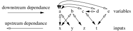
(b) Dependences forest

(c) Date propagation

Figure 3: The dependence forest and propagation law application for a specific equation system.The different pert levels are specified on the left hand side of figure 3(c).

We illustrate, the sorting algorithm we built on an example. Let us consider the set of equations expressed in figure 3(a). After the first step, we obtain the dependencies forest described in figure 3(b), Then, we perform early and late dates propagation. Initially, all variables are considered independent and their dates (early , late) are set to ($0$,$0$). The second step recursively propagates the Early Dates from the input and the register variables to the output variables and propagates the Late Dates from the output variables to the input and the register ones according to a n log n propagation algorithm. The algorithm that implements this second phasis is detailed in appendix B.2. Following the example presented in figure 3(a), the algorithm results in the dependencies described in figure 3(c).

5.2.2 Linking two Partial Orders

The approach allows an efficient merge of two already sorted equation systems, useful to perform separate compilation. To link the forest computed for module 1 with the forest computed for module 2, we don’t need to launch again the sorting algorithm from its initial step. In fact, it is sufficient to only adjust the $early(late)\ dates$ of the common variables to both equation systems and their dependencies. Notice that the linking operation applies $\xi$-algebra plus operator to merge common equations (i.e equations which compute the same variable). Then, we need to adjust evaluation dates: every output variable of module 1 propagates new $late\ date$ for every downstream variables. Conversely, every input variable of module 2 propagates new $early\ date$ for every upstream variables.

5.3 Practical Issues

We have mainly detailed the theoretical aspect of our approach, and in this section we will discuss the practical issues we have implemented.

5.3.1 Effective compilation

Relying on the equational semantic, we compile a le program into a $\xi$-algebra equation system. We call the compilation tool that achieves such a task clem (Compilation of LE Module). In order to perform separate compilation of le programs, we define an internal compilation format called lec (le Compiled code). This format is highly inspired from the Berkeley Logic Interchange Format (blif ). This latter is a very compact format to represent netlists and we just add to it syntactic means to record the early date and late date of each equation. Practically, clem compiler, among other output codes, generates lec format in order to reuse already compiled code in an efficient way, thanks to the pert algorithm we implement.

5.3.2 Effective Finalization

Our approach to compile le programs into a sorted $\xi$ equation system in an efficient way requires to be completed by what we call a finalization phasis to be effective. To generate code for simulation, verification or evaluation, we must start from a valid boolean equation systems, i.e we consider only equation systems where no event has value $\top$, since that means there is an error an we propagate this value to each element of the environment in the semantic previously described. Validity also means well sorted equation systems, to avoid to deal with programs having causality cycle. But in our approach we never set input event status to $absent$. Hence, we introduce a finalization operation which replaces all $\bot$ input events by $absent$ events and propagates this information in all equations related to local variables and outputs. Notice that the finalization operation is harmless. The sorting algorithm relies on propagation of signal status, and the substitution of $\bot$ by $absent$ cannot change the resulting sorted environment.

Let us illustrate the finalization mechanism on an example. In the following code $O1$ and $O2$ depends on the I status:

loop {
  present I {emit O1} else {emit O2}
  >> pause
}

Before finalization, we get the following equation system:

$O1_{def}=I_{def}$

$O1_{val}=I_{val}.I_{def}$

$O2_{def}=I_{def}$

$O2_{val}=\neg I_{val}.I_{def}$

We can see that $O1_{def}$ and $O2_{def}$ are not constant because $I$ is not necessarily defined for each instant (i.e $I_{def}$ can be $0$ if $I$ is $\bot$). After finalization $I_{def}$ is set to $1$ and $I_{val}$ remains free. According to the mapping from $\xi$ algebra to $\leavevmode\mbox{I}\!\mbox{B}\times\leavevmode\mbox{I}\!\mbox{B}$, an event $X$ such that $X_{def}=0$ is either $\top$ or $\bot$. Since, we discard equation systems where an event has value $\top$, To switch from $\bot$ value to $absent$ value, it is sufficient to set the $def$ part of a variable to 1. Now for each logical instant the status (present, absent) of I is known. The $O1$ and $O2$ equations become:

$O1_{def}=1$

$O1_{val}=I_{val}$

$O2_{def}=1$

$O2_{val}=\neg I_{val}$

We bring together compilation and finalization processus in a tool named clef(Compilation of LE programs and Finalization).

5.3.3 Compilation scheme

Figure 4: Compilation Scheme

Now, we detail the toolkit we have to specify, compile , simulate and execute le programs. A le file can be directly written. In the case of automaton, it can be generated by automaton editor like galaxy too. Each le module is compiled in a lec file and includes one instance of the run module references. These references can be already compiled in the past by a first call of the clem compiler. When the compiled process will done, the finalization will simplify the final equations and generate a file in the target use: simulation, safety proofs, hardware description or software code. That is summed up in the figure 4.

5.4 Benchmark

To complement the experimentation of the example, we have done some tests about the clem compiler. So we are interested in the evolution of the generated code enlarging with respect to the number of parallel processes increasing. A good indicator is the number of generated registers. Indeed, with $n$ registers, we can implement $2^{n}$ states in an automaton.

The chosen process is very simpler, not to disturb the result:

module WIO:
Input: I; Output: O;
wait I >> emit O
end

which waits the I signal and emits the signal O one time as soon as I occurs. Here is the obtained table by the figure 5:

Figure 5: Evolution of the Registers number

The relation between numbers of processes and number of registers seems to be linear, that is an excellent thing! The linear observed factor of $5$ is only characterized by the equational semantic of parallel and run statements. In a next equationnal semantic, this number should be reduced.

6 Example

We illustrate le usage on an industrial example concerning the design of a mecatronics process control: a pneumatic prehensor. We first describe how the system works. Then we present the system implementation with le language. Finally, simulation and verification are performed.

6.1 Mecatronics System Description

A pneumatic prehensor takes and assembles cogs and axes. The physical system mainly consists of two double acting pneumatic cylinders and a suction pad. This example has been taken as a benchmark by an automation specialist group, to experiment new methods of design and analysis of discrete event systems. The (U cycle) kinematics of the system is described in Fig.6. Note that the horizontal motion must always be done in the high position.

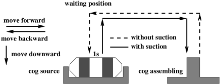
Figure 6: A pneumatic prehensor

The horizontal motion pneumatic cylinder is driven by a bistable directional control valve (bistable dcv). The associated commands are MoveFor (short for move forward) and MoveBack (short for move backward). The vertical cylinder is driven by a monostable directional control valve 5/2 whose active action is MoveDown (move downward). In the absence of activation, the cylinder comes back to its origin position (high position). The suction pad (SuckUp command) is activated by a monostable dcv (the suction is done by a Venturi effect).

Figure 7: Input/output signals

6.2 Mecatronics System LE Implementation

In what follow we consider the control part of the system. Fig.7 gathers incoming information (from the limit switches associated with the cylinders) and outgoing commands (to the pre-actuators). To implement this application in le language, we adopt a top down specification technique. At the highest hierarchical level , the controller is the parallel composition of an initialization part followed by the normal cycle running and a temporisation module. This last is raised by a signal start_tempo and emits a signal end_tempo when the temporisation is over. Of course, these two signals are not in overall interface of the controller, they are only use to establish the communication between the two parallel sides. The following le program implements the high level part of the controller:

module Control:

Input:forward, backward, upward,  downward,
      StartCycle;
Output:MoveFor, MoveBack, MoveDown, SuckUp,
       EndCycle ;

Run: "./TEST/control/" : Temporisation;
     "./TEST/control/" : NormalCycle;

local start_tempo, end_tempo {
   { wait upward >> emit MoveFor
     >> wait backward >> run NormalCycle
   }
 ||
   { run Temporisation}
}
end

The second level of the specification describes temporisation and normal cycle phasis. Both Temporisation and NormalCycle modules are defined in external files. Temporisation module performs a delaying operation (waiting for five successive reactions and then emitting a signal end_tempo. The overall le code is detailed in appendix C. In this section, we only discuss the NormalCycle module implementation. NormalCycle implementation is a loop whose body specifies a single cycle. According to the specification, a single cycle is composed of commands to move the pneumatic cylinders with respect to their positions and a call to a third level of implementation (Transport) to specify the suction pad activity.

module Transport :

Input: end_tempo, upward, forward, downward;
Output: MoveFor, MoveDown, SuckUp;

local exitTransport {

    { emit MoveDown >> wait end_tempo
      >> wait upward >> emit MoveFor
      >> wait forward >> emit MoveDown
      >> wait downward >> emit exitTransport
    }
 ||

    abort
      { loop { pause >> emit SuckUp }}
    when exitTransport
}

end

module NormalCycle :

Input:  StartCycle, downward, upward, backward,
        forward, end_tempo;
Output: start_tempo, MoveDown, MoveBack,
        MoveFor, SuckUp, EndCycle;

{ present StartCycle { nothing} else wait StartCycle}

>>

{
  loop { emit MoveDown
         >> wait downward >> emit start_tempo
         >> run Transport
         >> wait upward >> emit MoveBack
         >> wait backward >> emit EndCycle }
}
end

To compile the overall programs, we performed a separate compilation: first, Temporisation and NormalCycle modules have been compiled and respectively saved in lec format file. Second, the main Control module has been compiled according to our compilation scheme (see figure 4).

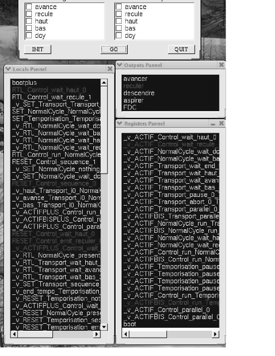
Figure 8: Control module simulation panels

6.3 Mecatronics System Simulation and Verification

To check the behavior of our implementation with respect to the specification, we first simulate it and then perform model-checking verification. Both simulation and verification relies on the generation of blif format from clem compiler.

Figure 8 shows the result of Control simulation with a graphical tool we have to simulate blif format modules.

On another hand, to formally prove safety properties we rely on model checking techniques. In this approach, the correctness of a system with respect to a desired behavior is verified by checking whether a structure that models the system satisfies a formula describing that behavior. Such a formula is usually written by using a temporal logic. Most existing verification techniques are based on a representation of the concurrent system by means of a labeled transition system (LTS). Synchronous languages are well known to have a clear semantic that allows to express the set of behaviors of program as LTSs and thus model checking techniques are available. Then, they rely on formal methods to build dependable software. The same occurs for le language, the LTS model of a program is naturally encoded in its equational semantic.

A verification means successfully used for synchronous formalisms is that of observer monitoring [10]. According to this technique, a safety property $\phi$ can be mapped to a program $\Omega$ which runs in parallel with a program P and observes its behavior, in the sense that at each instant $\Omega$ reads both inputs and outputs of P. If $\Omega$ detects that P has violated $\phi$ then it broadcasts an "alarm" signal. As a consequence, we can rely on model checking based tools to verify property of le language. But, our approach provides us with separate compilation and requires to be completed by a modular verification. We aim at proving safety properties are preserved through le language operator application.

To verify that the suction is maintained from the instant where the cycle begins up to the cycle ends, the following observer can be written in le .

module CheckSuckUp;
Input SuckUp, S;
Output exitERROR;
present SuckUp
        { present S {nothing} else {wait S}}
        else {pause>>emit exitERROR}
end

module SuctionObs:

Input:forward, backward, upward,  downward,
      StartCycle, Output:MoveFor, MoveBack,
      MoveDown, SuckUp, EndCycle ;
Output: ERROR;

local exitERROR {
 abort {
  loop {
   present StartCycle {nothing}
           else {wait StartCycle} >>
   present MoveDown {nothing}
                    else {wait MoveDown}  >>
   present downward {nothing}
                    else { wait downward} >>
   present MoveDown {nothing}
           else { present SuckUp
                     {run CheckSuckUp[upward\S]   >>
                      run CheckSuckUp[MoveFor\S]  >>
                      run CheckSuckUp[forward\S]  >>
                      run CheckSuckUp[MoveDown\S] >>
                      wait downward
                     }
                     else {emit exitERROR}
                }
  }
 when exitERROR >> emit ERROR
 }
}
end

To specify the observer we first define a module (CheckSuckUp) which checks wether the signal SuckUp is present and goes in the state where signal S is present. If SuckUp is absent , exitERROR is emitted. Calling this module, the observer tests the presence of signal SuckUp in each possible states reached when cylinders move.

To achieve the property checking, we compile a global module made of the Control module in parallel with the SuctionObs module and we rely on model checker to ensure that ERROR is never emitted. By the time, we generate the blif format back end for the global module and we call xeve model-checker [4] to perform the verification. In the future, we intend to interface NuSMV [5] model-checker.

The chosen example is a very simple one but we hope understandable in the framework of a paper. Nevertheless, we compiled it globally and in a separate way. The global compilation takes about 2.7 s while the separate one takes 0.6 s on the same machine. We think that it is a small but promising result.

7 Conclusion

In this work, we have presented a new synchronous language le that supports separate compilation. We defined its behavioral semantic giving a meaning to each program and allowing us to rely on formal methods to achieve verification. Then, we also defined an equational semantic to get a means to really compile programs in a separate way. Actually, we have implemented the clem/clef compiler. This compiler is the core of the design chain (see section 5.3.3) we have to specify control-dominated process from different front-ends: a graphical editor devoted to automata drawing, or direct le language specification to several families of back-ends:

• code generation: we generate either executable code as C code or model-driven code: Esterel, Lustre code for software applications and Vhdl for harware targets.

• simulation tools: thanks to the blif format generation we can rely our own simulator (blif_simul) to simulate le programs.

• verification tools: blif is a well-suited format to several model-checkers(xeve, sis) and has its automata equivalence verifier (blif2autom, blifequiv).

In the future, we will focus on three main directions. The first one concerns our compilation methodology. Relying on an equational semantic to get modular compilation could lead to generate inefficient code. To avoid this drawback, we plan to study others equational semantic rules (in particular for parallel and run statements) more suited for optimization. The second improvement we aim at, is the extension of the language. To be able to deal with control-dominated systems with data (like sensor handling), we will extend the syntax of the language on the first hand. On the other hand, we plan to integrate abstract interpretation techniques (like polyhedra intersection, among others) [6] to take into account data constraints in control. Moreover, we also need to communicate with signal processing or automation world through their specific tool Matlab/Simulink (http://www.mathworks.com). Another language extension is to allow a bound number of parallel operators. This extension is frequently required by users to specify their applications. Semantic rules for this new bound parallel operator cannot be straightly deduced from the actual rules we have, and require a deep change but then would improve le expressiveness. Finally, we are interested in improving our verification means. The synchronous approach provides us with well-suited models to apply model checking techniques to le programs. The more efficient way seems to directly interface a powerful model-ckecker (as NuSMV [5]) and to be able to run its property violation scenarios in our simulation tool. Moreover, our modular approach opens new ways to modular verification. We need to prove that le operators preserve properties: if a program $P$ verify a property $\phi$, then all program using $P$ should verify a property $\phi^{\prime}$ such that the “restriction” of $\phi^{\prime}$ to $P$ implies $\phi$.

Appendix A LE Grammar

In this appendix, we describe the complete grammar of the le language. That description supports the following agreements:

• <> notation represents tokens, for instance <module> represents the name module;

• two specific tokens are introduced: IDENT for identifier and STRING to denote a usual string;

• the notation $\star$ and $+$ are used for repetition: $signal\_name\star$ means a number of $signal\_name$, possibly 0,while $signal\_name+$ means at least one occurrence;

• the single charater are straighly written (as {,},[,], and $\backslash$).

• the character # denotes the empty word;

program: <module> module_name ’:’ module_interface module_body <end>;

module_interface : input_signal_list output_signal_list run_decl_list;

input_signal_list : # | <Input:> signal_name+ ’;’ ;
output_signal_list : #  | <Output:> signal_name+ ’;’ ;
run_decl_list : #  | <Run:> run_declaration+ ;
run_declaration: path ’:’ module_name;

module_body : instruction | automaton ;

instruction : statement | ’{’ instruction ’}’ ;

statement : parallel
          | sequence
          | present
          | loop
          | wait
          | emit
          | abort
          | nothing
          | pause
          | halt
          | local
          | run
          ;

parallel : instruction ’||’ instruction ;
sequence :  instruction ’>>’ instruction ;
present : <present> xi_expression  instruction   <else> instruction ;
loop :  <loop> ’{’ instruction ’}’ ;
wait :   <waitL>  signal_name ;
emit : <emit> signal_name ;
abort : <abort> ’{’ instruction ’}’ <when> signal_name ;
pause : <pause> ;
nothing : <nothing> ;
halt : <halt> ;
local :  <local> signal_name+ ’{’ instruction ’}’
run : <run> module_name  renaming ;
renaming : #  | ’[’ single_renaming+ ’]’ ;
single_renaming :  signal_name ’\’ signal_name


automaton : <automaton> state+ transition_def ;
state : <state> state_name opt_final opt_run  action ’;’ ;
opt_run: #  | run ;
transition_def :  <transition> transition+ ;
transition : opt_initial opt_final  opt_source_state  trigger  action opt_target_state ;
opt_source_state: # | state_name;
opt_target_state: # | ’->’ state_name;
opt_initial : # | <initial> ;
opt_final:  # | <initial> ;
trigger:  # | xi_expression ;
action: # | ’/’ signal_name+ ;
xi_expression : xi_expression <or> xi_expression
              | xi_expression <and> xi_expression
              | <not> xi_expression
              | ’{’ xi_expression ’}’
              | signal_name
              ;

signal_name : IDENT;
module_name : IDENT;
path : STRING;

Appendix B PERT Algorithms

B.1 First Step of PERT ALGORITHM

The following algorithm is the first step of the overall PERT algorithm we implement. It builds a forest of variable dependency trees.

for each equation xi=fi(...,xj,...)
begin
   for all j needed by fi
   begin
      Upstream[i].add(j);
      Downstream[j].add(i)
   end
end

B.2 Second Step of PERT Algorithm

The second step of the PERT algorithm we implement consists in the propagation of the Early Dates from the inputs and the registers, to the outputs. Similarly, the Late Dates are propagated from the outputs to the inputs and the registers according to the following algorithm:

for each variable id i
begin
   if(Upstream[i] = empty set)
   begin
      /* final output */
      late[i]=0
      for each j in Downstream[i]
      begin
         late_propagation(j,1)
      end
   end
   if(Downstream[i] = empty set)
   begin
      /* real input or constante */
      early[i]=0
      for each j in Upstream[i]
      begin
         early_propagation(j,1)
      end
   end
end

function late_propagation(id,date)
begin
  if(late[id] < date)
  begin
    late[id]=date
    for each j in Dowstream[id]
    begin
       late_propagation(j,date+1)
    end
  end
end

function early_propagation(id,date)
begin
  if(early[id] < date)
  begin
    early[id]=date
    for each j in Upstream[id]
    begin
       early_propagation(j,date+1)
    end
  end
end

Appendix C LE Control Example Code

In this appendix, we detail the le code for the Control example described in section 6.

C.1 Control Module Specification

The main file of the Control example is Control.le. We give its content:

;;====================================================
;; LE specification for a mecatronic system
;; Main file: Control specification
;;====================================================


module Control:

Input:  forward, backward, upward, downward, StartCycle;
Output: MoveFor, MoveBack, MoveDown, SuckUp, EndCycle;

Run: "/home/ar/GnuStrl/work-ar/TEST/control/" : Temporisation;
     "/home/ar/GnuStrl/work-ar/TEST/control/" : NormalCycle;

local start_tempo, end_tempo {

     { wait upward >> emit MoveBack >> wait backward >> run NormalCycle}
  ||
     { run Temporisation}
}

end

The Control module calls two external modules Temporisation and NormalCycle. The paths to Temporisation.le and NormalCycle.le files where the respective le codes of these called modules are, is given in Control module interface. During compilation, a file temporisation.lec (resp NormalCyle.lec) is searched in the compilation library. If Temporisation (resp NormalCycle) has not been already compiled then it is compiled. Thus, in both cases, the compiled code is included in Control module code.

C.2 Temporisation module Specification

;;====================================================
;; LE specification for a mecatronic system
;; Temporisation  specification
;;====================================================

module Temporisation :

Input:  start_tempo;
Output: end_tempo;

present start_tempo {
 pause >> pause >> pause >> pause >> emit end_tempo }
else nothing

end

C.3 NormalCycle module Specification

;;====================================================
;; LE specification for a mecatronic system
;; Normal cycle  specification
;;====================================================

module Transport :

Input: end_tempo, upward, forward, downward;
Output: MoveDown,MoveFor, SuckUp;

local exitTransport {

    { emit MoveDown >> wait end_tempo >> wait upward >> emit MoveFor
      >> wait forward >> emit MoveDown >> wait downward  >> emit exitTransport
    }
 ||

    abort
      { loop { pause >> emit SuckUp }}
    when exitTransport
}

end

module NormalCycle :

Input: StartCycle, downward, upward, backward, end_tempo, forward;
Output: start_tempo, MoveDown,MoveBack, EndCycle, MoveFor, SuckUp;

{ present StartCycle { nothing} else wait StartCycle }

>>

{
  loop { emit MoveDown >> wait downward >> emit start_tempo  >> run Transport
         >> wait upward >> emit MoveBack
         >> wait backward >> emit EndCycle }
}

end

The NormalCycle module called itself a Transport module, but contrary to Control module, the specification of the called module is given in the same file. Thus, no path has to be supplied in NormalCycle interface.

Appendix D Condition Law Expansion

In this appendix, we discuss how a term from $\xi$ algebra resulting of the application of the condition law is expanded in a pair of boolean values in IB.. Let us consider a $\xi$ term $X$. We recall that $X$ is isomorphic to a pair of boolean ($X_{def}$, $X_{va;}$) (see section 3.1) and we want to prove the following equalities: $(X\blacktriangleleft c)_{def}=X_{def}.c$ and $(X\blacktriangleleft c)_{val}=X_{val}.c$, where $c\in\leavevmode\mbox{I}\!\mbox{B}$.

These equalities are very useful for implementing the condition law in the compilation phasis.

First, relying on the definition of the isomorphism between $\xi$ algebra and $\leavevmode\mbox{I}\!\mbox{B}\times\leavevmode\mbox{I}\!\mbox{B}$, we can expand the encoding of the condition law as follow:

$X$	$X_{def}$	$X_{val}$	$c$	$(X\blacktriangleleft c)$	$(X\blacktriangleleft c)_{def}$	$(X\blacktriangleleft c)_{val}$
1	1	1	0	$\bot$	0	0
0	1	0	0	$\bot$	0	0
$\top$	0	1	0	$\bot$	0	0
$\bot$	0	0	0	$\bot$	0	0
1	1	1	1	1	1	1
0	1	0	1	0	1	0
$\top$	0	1	1	$\top$	0	1
$\bot$	0	0	1	$\bot$	0	0

where $c\in\leavevmode\mbox{I}\!\mbox{B}$.

Thus, we can deduce:

$(X\blacktriangleleft c)_{def}$	= $X_{def}.X_{val}.c\ +\ X_{def}.\overline{X_{val}}.c$
	$=X_{def}.c.(X_{val}+\overline{X_{val}})$
	$=X_{def}.c$
$(X\blacktriangleleft c)_{val}$	= $X_{def}.X_{val}.c\ +\ \overline{X_{def}}.X_{val}.c$
	$=X_{val}.c.(X_{def}+\overline{X_{def}})$
	$=X_{val}.c$

Appendix E LE Statement Circuit Description

In this appendix, we show the circuits corresponding to le statement. We rely on them to compute the equational semantic of each le operator.

(a) Circuit for nothing

(b) Circuit for halt

Figure 9: Basic le statements circuit semantic

Figure 10: Circuit for emit$S$

(a) Circuit for pause

(b) Circuit for wait

Figure 11: Pause and Wait le statements circuit semantic

Figure 12: Circuit for $\texttt{\small{Present}}\ S\{{\rm P}_{1}\}\texttt{\small{else}}\{{\rm P}_{2}\}$

Figure 13: Circuit for${\rm P}_{1}\|{\rm P}_{2}$

Figure 14: Circuit for ${\rm P}_{1}\gg{\rm P}_{2}$

Figure 15: Circuit for abort P when $S$

Figure 16: Circuit for loop {P}

Figure 17: Circuit for run{P}

Figure 18: Circuit for ${\cal A}({\rm M}_{\rm init},..,{\rm M},...,{\rm M}_{\rm final})$

References

- [1] C. André, H. Boufaïed, and S. Dissoubray. Synccharts: un modèle graphique synchrone pour système réactifs complexes. In Real-Time Systems(RTS’98), pages 175–196, Paris, France, January 1998. Teknea.
- [2] G. Berry. The Constructive Semantics of Pure Esterel. Draft Book, available at: http://www.esterel-technologies.com 1996.
- [3] G. Berry. The Foundations of Esterel. In G. Plotkin, C. Stearling, and M. Tofte, editors, Proof, Language, and Interaction, Essays in Honor of Robin Milner. MIT Press, 2000.
- [4] Amar Bouali. Xeve , an esterel verification environment. Technical report, CMA-Ecole des Mines, 1996.
- [5] A. Cimatti, E. Clarke, E. Giunchiglia, F. Giunchiglia, M. Pistore, M. Roveri, R. Sebastiani, and A. Tacchella. NuSMV 2: an OpenSource Tool for Symbolic Model Checking. In Ed Brinksma and Kim Guldstrand Larsen, editors, Proceeeding CAV, number 2404 in LNCS, pages 359–364, Copenhagen, Danmark, July 2002. Springer-Verlag.
- [6] P. Cousot and R. Cousot. On Abstraction in Software Verification. In Ed Brinksma and Kim Guldstrand Larsen, editors, Proceeeding CAV, number 2404 in LNCS, pages 37,56, Copenhagen, Danmark, July 2002. Springer-Verlag.
- [7] S.A. Edwards. Compiling esterel into sequential code. In Proceedings of the 7th International Workshop on Hardware/Software Codesign (CODES 99), pages 147–151, Rome, Italy, May 1999.
- [8] M. Gordon. The Denotational Description of Programming Languages. Springer-Verlag, 1979.
- [9] N. Halbwachs. Synchronous Programming of Reactive Systems. Kluwer Academic, 1993.
- [10] N. Halbwachs, F. Lagnier, and P. Raymond. Synchronous observers and the verification of reactive systems. In M. Nivat, C. Rattray, T. Rus, and G. Scollo, editors, Third Int. Conf. on Algebraic Methodology and Software Technology, AMAST’93, Twente, June 1993. Workshops in Computing, Springer Verlag.
- [11] D. Harel and A. Pnueli. On the development of reactive systems. In NATO, Advanced Study institute on Logics and Models for Verification and Specification of Concurrent Systems. Springer Verlag, 1985.
- [12] C. Huizing and R. Gerth. Semantics of reactive systems in abstract time. In Real Time: Theory in Practice, Proc of REX workshop, pages 291–314. W.P. de Roever and G. Rozenberg Eds,LNCS, June 1991.
- [13] D. Potop-Butucaru and R. De Simone. Formal Methods and Models for System Design, chapter Optimizations for Faster Execution of Esterel Programs. Gupta, P. LeGuernic, S. Shukla, and J.-P. Talpin, Eds ,Kluwer, 2004.
- [14] T. Shiple. Formal Analysis of Cyclic Circuits. PhD thesis, University of California, 1996.
- [15] Esterel Technologies. Esterel studio suite, www.estereltechnologies.com.
- [16] D. Weil, V. Bertin, E. Closse, M. Poize, P. Venier, and J. Pulou. Efficient compilation of esterel for real-time embedded systems. In Proceedings of the 2000 International Conference on Compilers, Architecture, and Synthesis for Embedded Systems,, pages 2–8, San Jose, California, United States, November 2000.