Joint source and channel coding for MIMO systems:
Is it better to be robust or quick?

Abstract

We develop a framework to optimize the tradeoff between diversity, multiplexing, and delay in MIMO systems to minimize end-to-end distortion. The goal is to find the optimal balance between the increased data rate provided by antenna multiplexing, the reduction in transmission errors provided by antenna diversity and automatic repeat request (ARQ), and the delay introduced by ARQ. We first focus on the diversity-multiplexing tradeoff in MIMO systems, and develop analytical results to minimize distortion of a vector quantizer concatenated with a space-time MIMO channel code. In the high SNR regime we obtain a closed-form expression for the end-to-end distortion as a function of the optimal point on the diversity-multiplexing tradeoff curve. For large but finite SNR we find this optimal point via convex optimization. The same general framework can also be used to minimize end-to-end distortion for a broad class of practical source and channel codes, which we illustrate with an example.

We then consider MIMO systems using ARQ retransmission to provide additional diversity at the expense of delay. We show that for sources without a delay constraint, distortion is minimized by maximizing the ARQ window size. This results in an ARQ-enhanced multiplexing-diversity tradeoff region, with distortion minimized over this region in the same manner as without ARQ. However, under a source delay constraint the problem formulation changes to account for delay distortion associated with random message arrival and random ARQ completion times. Moreover, the simplifications associated with a high SNR assumption break down for this analysis, since retransmissions, and the delay they cause, become rare events. We thus use a dynamic programming formulation to capture the channel diversity-multiplexing tradeoff at finite SNR as well as the random arrival and retransmission dynamics. This fomulation is used to solve for the optimal multiplexing-diversity-delay tradeoff to minimize end-to-end distortion associated with the source encoder, channel, and ARQ retransmissions. Our results show that a delay-sensitive system should adapt its operating point on the diversity-multiplexing-delay tradeoff region to the system dynamics. We provide numerical results that demonstrate significant performance gains of this adaptive policy over a static allocation of diversity/multiplexing in the channel code and a static ARQ window size.

Keywords: ARQ, diversity-multiplexing-delay tradeoff, joint source-channel coding, MIMO channels.

I Introduction

Multiple antennas can significantly improve the performance of wireless systems. In particular, with channel knowledge at the receiver a data rate increase equal to the minimum number of transmit/receive antennas can be obtained by multiplexing data streams across the parallel channels associated with the channel gain matrix. Alternatively, multiple antennas enable transmit and/or receive diversity which decreases the probability of error. In a landmark result Zheng and Tse [27] developed a rigorous fundamental tradeoff between the data rate increase possible via multiplexing versus the channel error probability reduction possible via diversity, characterizing how a higher spatial multiplexing gain leads to lower diversity and vice versa. The main result in [27] is an explicit characterization of the diversity-multiplexing tradeoff region. This result generated much activity in finding diversity-multiplexing tradeoffs for other channel models as well as design of space-time codes that achieve any point on the tradeoff region [1, 8, 6, 16, 18, 24]. The diversity-multiplexing tradeoff was also extended to the multiple access channel in [23]. Delay provides a third dimension in the tradeoff region, and this dimension was explored for MIMO channels based on the automatic repeat request (ARQ) protocol in [7]. In particular, this work characterized the three-dimensional tradeoff between diversity, multiplexing, and ARQ-delay for MIMO systems.

Our goal in this paper is to answer the following question: “Given the diversity-multiplexing-delay tradeoff region, where should a system operate on this region?”. In order to answer this question we require a performance metric from a layer above the physical layer; while physical layer tradeoffs are based on the channel model, the optimization between these tradeoffs depends on what is most important for the application’s end-to-end performance. The higher layer metric of interest in this paper will be end-to-end distortion. Specifically, our system model consists of a lossy source encoder concatenated with a MIMO channel encoder and, in the last section, an ARQ retransmission protocol. Our goal is to determine the optimal point on the diversity-multiplexing or diversity-multiplexing-delay tradeoff region that minimizes the combined distortion due to the source compression, channel, and delays in the end-to-end system.

Our problem formulation differs from the Shannon-theoretic joint source-channel coding problem in that we do not assume asymptotically long block lengths for either the source or channel code. In particular, the traditional joint source/channel code formulation assumes stationary and ergodic sources and channels in the asymptotic regime of large source dimension and channel code blocklength. Shannon showed that under these assumptions the source should be encoded at a rate just below channel capacity and then transmitted over the channel at this rate. Since the rate is less than capacity, the channel introduces negligible error, hence the end-to-end distortion equals the distortion introduced by compressing the source to a rate below the channel capacity. Shannon’s well-known separation theorem indicates that this transmission scheme is optimal for minimizing end-to-end distortion and does not require any coordination between the source and channel coders or decoders other than agreeing on the channel transmission rate [4, 5].

Our joint source/channel code formulation is fundamentally different from Shannon’s since we assume a finite blocklength for the channel code. This assumption is inherent to the diversity-multiplexing tradeoff since, without finite blocklength, the channel introduces negligible error and hence the diversity gain in terms of channel error probability is meaningless. The finite blocklength guarantees there is a nonnegligible probability of error in the channel transmission. Thus there is a tradeoff between resolution at the source encoder and robustness at the channel encoder: limiting source distortion requires a high-rate source code, for which the multiple antennas of the channel must be used mainly for multiplexing. Alternatively, the source can be encoded at a lower rate with more distortion, and then the channel error probability can be reduced through increased diversity. Our joint source/channel code must determine the best tradeoff between these two to minimize end-to-end distortion. When retransmission is possible and the source is delay-sensitive, there is an additional tradeoff between reducing channel errors through retransmissions versus the delay these retransmissions entail.

Joint source/channel code optimization for the binary symmetric channel (BSC) with finite blocklength channel codes and asymptotically high source dimension was previously studied in [15]. We will use several key ideas and results from this prior work in our asymptotic analysis, in particular its decomposition of end-to-end distortion into separate components associated with either the source code or the channel code. By applying this decomposition to MIMO channels instead of the BSC, we obtain the optimal operating point on the Zheng/Tse diversity-multiplexing tradeoff region in the asymptotic limit of high source dimension and channel SNR. For any SNR the MIMO channel under multiplexing can be viewed as a parallel channel, and source/channel coding for parallel channels has been previously explored in [17]. That work differs from ours in that the source models were not high dimensional and the nonergodic parallel channels did not have the same diversity-multiplexing tradeoff characterization as in a MIMO system.

We first develop a closed-form expression for the optimal “distortion exponent”, introduced in [17], under asymptotically high SNR. Specifically, for a multiplexing rate $r$ and average distortion measure $D(r)$ we compute

$$d_{D}^{*}=\min_{r}\left[\lim_{\mathrm{SNR}\rightarrow\infty}\frac{\log\bar{D}(r)}{\log\mathrm{SNR}}\right],$$ (1)

where $d_{D}^{*}$ is the optimal exponential rate at which the distortion goes to zero with SNR. We show that the optimal distortion exponent corresponds to a particular point on the diversity-multiplexing tradeoff curve that is determined by the source characteristics. We also demonstrate there is no loss in optimality for separate source and channel encoding and decoding given the channel transmission rate. Our optimization framework can also be used to optimize the diversity-multiplexing tradeoff at finite SNR, however the solution is no longer in closed-form and must be found using tools from convex optimization. We extend this general optimization framework to a wide variety of practical source-channel codes in non-asymptotic regimes.

We next consider the impact of ARQ retransmissions and their associated delay. When the source does not have a delay constraint, the ARQ delay incurs no cost in terms of additional distortion. Hence, the ARQ protocol should use the maximum window size to enhance the diversity-multiplexing tradeoff region associated with the MIMO channel alone. The large window size essentially allows coding over larger blocklengths than without ARQ, which from Shannon theory does not reduce data rate, only probability of error. In the high SNR regime the optimal distortion exponent for the diversity-multiplexing tradeoff region enhanced by ARQ is found in the same manner as without ARQ. Not surprisingly, a delay constraint on the source changes the problem considerably, since the source burstiness and queuing delay must now be incorporated into the problem formulation. These characteristics are known to be a significant obstacle in merging analysis of the fundamental limits at the physical layer with end-to-end network performance [10]. In this setting the simplicity associated with the high SNR regime breaks down, since at high SNR retransmissions and their associated delay have very low probability, which essentially removes the third dimension of delay in our tradeoff region. We thus use dynamic programming to model and optimize over the system dynamics as well as the fundamental physical layer tradeoffs to minimize end-to-end distortion of a MIMO channel with ARQ.

The remainder of this paper is organized as follows. In the next section we present the channel model and summarize the diversity-multiplexing tradeoff results from [27]. In Section III we develop our source encoding framework and apply the MIMO channel error probability results of [27] to the upper and lower bounds on end-to-end distortion of [15]. Section IV obtains a closed-form expression for the optimal operating point on the MIMO channel diversity-multiplexing tradeoff curve in the high SNR regime to minimize end-to-end distortion. This optimal point is also found for large, but finite, SNR using convex optimization. In Section V we present a similar formulation for optimizing diversity and multiplexing in progressive video transmission using space-time codes. ARQ retransmission and its corresponding delay is considered in Section VI, where a dynamic programming formulation is used to optimize the operating point on the diversity-multiplexing-delay tradeoff region for minimum end-to-end distortion of delay-constrained sources. A summary and closing thoughts are provided in Section VII.

II Channel Model

We will use the same channel model and notation as in [27]. Consider a wireless channel with $M$ transmit antennas and $N$ receive antennas. The fading coefficients $h_{ij}$ that model the gain from transmit antenna $i$ to receive antenna $j$ are independent and identically distributed (i.i.d.) complex Gaussian with unit variance. The channel gain matrix $\mathbf{H}$ with elements $H(i,j)=(h_{ij}:i\in\{1,\ldots M\},j\in\{1,\ldots,N\})$ is assumed to be known at the receiver and unknown at the transmitter. We assume that the channel remains constant over a block of $T$ symbols, while each block is i.i.d. Therefore, in each block we can represent the channel as

$$\mathbf{Y}=\sqrt{\frac{\mathrm{SNR}}{M}}\mathbf{HX}+\mathbf{W},$$ (2)

where $\mathbf{X}\in\mathcal{C}^{M\mathrm{x}T}$ and $\mathbf{Y}\in\mathcal{C}^{N\mathrm{x}T}$ are the transmitted and received signal vectors, respectively. The additive noise vector $\mathbf{W}$ is i.i.d. complex Gaussian with unit variance.

We construct a family of codes for this channel $\{C(\mathrm{SNR})\}$ of block length $T$ for each $\mathrm{SNR}$ level. Define $P_{e}(\mathrm{SNR})$ as the average probability of error and $R(\mathrm{SNR})$ as the number of bits per symbol for the codebook. A channel code scheme $\{C(\mathrm{SNR})\}$ is said to achieve multiplexing gain $r$ and diversity gain $d$ if

$$\lim_{\mathrm{SNR}\rightarrow\infty}\frac{R(\mathrm{SNR})}{\log_{2}\mathrm{SNR}}=r,$$ (3)

and

$$\lim_{\mathrm{SNR}\rightarrow\infty}\frac{\log_{2}P_{e}(\mathrm{SNR})}{\log_{2}\mathrm{SNR}}=-d.$$ (4)

All logarithms we consider will have base 2 and we therefore suppress this base notation in the remainder of the paper. For each $r$ we define the optimal diversity gain $d^{*}(r)$ as the supremum of the diversity gain achieved by any scheme. The main result from [27] that we will use in the next section is summarized in the following statement.

Diversity-Multiplexing Tradeoff [27]: Assume the block length satisfies $T\geq M+N-1$. Then the optimal tradeoff between diversity gain and multiplexing gain is the piecewise-linear function connecting the points $d^{*}(r)=(M-r)(N-r)$, for integer values of $r$ such that $0\leq r\leq\min(M,N)$. This function $d^{*}(r)$ is plotted in Figure 1.

In the Zheng/Tse framework the rate of the codebook $\{C(\mathrm{SNR})\}$ must scale with $\log\mathrm{SNR}$, otherwise the multiplexing gain will go to zero. Hence, in the following sections we will assume, without loss of generality, that the rate of the codebook is $Tr\log\mathrm{SNR}$ for any choice of $0\leq r\leq\min(M,N)$ and block length $T$. We also assume that the codebook achieves the optimal diversity gain $d^{*}(r)$ for any choice of $r$. Codes achieving the optimal diversity-multiplexing tradeoff for MIMO channels have been investigated in many works, including [6, 8, 9, 20] and the references therein.

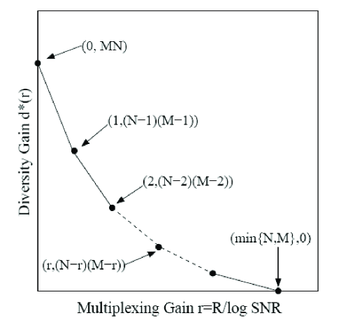
Figure 1: The optimal diversity-multiplexing tradeoff for $T\geq M+N-1$.

III End-to-End Distortion

This section presents our system model for the end-to-end transmission of source data. We use the same source coding model as [15] in order to exploit their decomposition of end-to-end distortion into separate source and channel distortion components. We assume the original source data $u$ is a random variable with probability density $h(u)$, which has support on a closed and bounded subset of $\Re^{k}$ with non-empty interior. An $s$-bit quantizer is applied to $u$ via the following transformation:

$$Q(u)=\sum_{i=1}^{2^{s}}v_{i}I_{[A_{i}]}(u),$$ (5)

where $I_{[A_{i}]}(u)=I[u\in A_{i}]$ is the standard indicator function, and $\{A_{i}\}_{i=1}^{2^{s}}$ is a partition of $\Re^{k}$ into disjoint regions. Each region $A_{i}$ is represented by a single codevector $v_{i}$. The $p$th-order distortion due to the encoding process is

$$D_{s}(Q)=\sum_{i=1}^{2^{s}}\int_{A_{i}}||u-v_{i}||^{p}h(u)du,$$ (6)

where $||u-v_{i}||^{p}$ is the $p$th power of the Euclidian norm.

We assume that the rate of the channel codebook $\mathcal{C}\{\mathrm{SNR}\}$ is matched to the rate of the quantizer (i.e. $s=Tr\log\mathrm{SNR}$). Each codevector from the quantizer $v_{1},\ldots,v_{{}_{2^{s}}}$ is mapped into a codeword from $\mathcal{C}\{\mathrm{SNR}\}$ through a permutation mapping $\pi$. We assume the mapping $\pi$ is chosen equally likely at random from the $2^{s}!$ possibilities. The codeword $\pi(i)$ is transmitted over the channel described in Section 2 and decoded at the receiver. Let $q(\pi(j)|\pi(i))$ be the probability that codeword $\pi(j)$ is decoded at the receiver given that $\pi(i)$ was transmitted. The probability $q(\cdot|\cdot)$ will depend on the $\mathrm{SNR}$, the quantizer $Q$’s codeword set, and the permutation mapping $\pi$. Hence, we can write the total end-to-end distortion as follows:

$$D_{\tau}(Q,\mathrm{SNR},\pi)=\sum_{i=1}^{2^{s}}\sum_{j=1}^{2^{s}}q(\pi(j)|\pi(i))\int_{A_{j}}||u-v_{j}||^{p}h(u)du.$$ (7)

Ideally we would like to be able to analyze the distortion averaged over all index assignments and possibly remove the dependence on $h$ and $Q$. In general we cannot find a closed form expression for this distortion due to the dependence on $Q$’s codewords, $\pi$, $h$, and the SNR. However, given our matched source and channel rate $s=Tr\log\mathrm{SNR}$, is clear that we have a tradeoff between transmitting at a high data rate to reduce source distortion and transmitting at a low data rate to reduce channel errors. In particular, if we run full multiplexing in the MIMO channel (i.e. set $r=\min(M,N)$) we can use a large $s$. This would result in low distortion at the source encoder but possibly create many transmission errors. Conversely, we could use full diversity in the channel (i.e. set $d=MN$) to combat errors and then suffer the distortion from a low value of $s$. Between the two extremes lies a source code rate $s$ and a corresponding channel multiplexing rate $r$ that minimizes (7).

Although we cannot find a simple general expression for $D_{\tau}(Q,\mathrm{SNR},\pi)$, in the following subsections we will determine tight asymptotic bounds for the distortion through the use of high-resolution source coding theory and high-SNR analysis of the MIMO channel. In addition, as the $\mathrm{SNR}$ approaches infinity we will find a simple expression for the optimal choice of $r$ and $s$ that depends only on the block length $T$, source dimension $k$, number of transmit antennas $M$, and number of receive antennas $N$.

The high-resolution asymptotic regime is often used in source coding theory to obtain analytical results, since the performance characteristics of many encoder types are well understood in this regime [26]. Moreover, it has been show that the high resolution asymptotics often provide a good approximation for non-asymptotic performance [19, 22]. As described in [26], we say that a quantizer $Q$ operates in the high-resolution asymptotic regime if its noiseless distortion asymptotically approaches

$$D_{s}(Q)=2^{-ps/k+O(1)},$$ (8)

as $s$ goes to infinity, where the $O(1)$ term in (8) may depend on $p$, $k$, and $s$. Many practical quantizers achieve this asymptotic distortion, e.g. uniform and lattice-based quantizers [3, 25]. This high-resolution asymptotic regime is quite accurate for our system model since we require the rate of our channel codebook $\{C(\mathrm{SNR})\}$ to scale as $r\log\mathrm{SNR}$. Hence, at asymptotically high SNR, the source coder will receive an increasing number of bits, thereby approaching its high-resolution regime.

In the next two subsections we will construct upper and lower asymptotic bounds for the end-to-end average distortion of our system. The starting point for both bounds comes from the analysis of [15]. In Section IV we will show that these bounds are tight and find the optimal multiplexing rate that minimizes distortion in the high SNR regime.

III-A Upper Bound for Distortion

We first construct an upper bound for the end-to-end distortion (7) that depends on $\pi$. As shown in [15],

$$D_{\tau}(Q,\mathrm{SNR},\pi) = \sum_{i=1}^{2^{s}}\sum_{j=1}^{2^{s}}q(\pi(j)|\pi(i))\int_{A_{i}}||u-v_{j}||^{p}h(u)du$$ (9)

$$= \sum_{i=1}^{2^{s}}q(\pi(i)|\pi(i))\int_{A_{i}}||u-v_{j}||^{p}h(u)du$$

$$+ \sum_{j,i=1,i\neq j}^{2^{s}}q(\pi(j)|\pi(i))\int_{A_{i}}||u-v_{j}||^{p}h(u)du$$

$$\leq \sum_{i=1}^{2^{s}}\int_{A_{i}}||u-v_{j}||^{p}h(u)du+O(1)\sum_{i=1}^{2^{s}}P(A_{i})\sum_{j=1,j\neq i}^{2^{s}}q(\pi(j)|\pi(i))$$

$$\leq D_{s}(Q)+O(1)\max_{i}P_{e|\pi(i)}(\mathrm{SNR}),$$

where $P_{e|\pi(i)}$ is the probability of codeword error given that codeword $\pi(i)$ was transmitted. This bound essentially splits (7) into two pieces; one corresponding to correctly received channel codewords and the other corresponding to erroneous channel decoding. The term corresponding to correct transmission is bounded by the noiseless distortion $D_{s}(Q)$ while the term corresponding to errors is bounded by a constant multiplied by the channel codeword error probability.

By construction, the rate of our channel codebook (and hence the source encoder) is $s=Tr\log\mathrm{SNR}$, therefore

$$D_{s}(Q)=2^{-ps/k+O(1)}=2^{-\frac{pTr}{k}\log\mathrm{SNR}+O(1)}$$ (10)

as $s$ approaches infinity or, equivalently, as $\log\mathrm{SNR}$ approaches infinity. In order to bound the probability of codeword error we need a few quantities from [27]. For the channel defined in (2), let $P_{out}(r\log\mathrm{SNR})$ and $d_{out}(r)$ be the outage probability and outage exponent that satisfy

$$P_{out}(r\log\mathrm{SNR})=2^{-d_{out}(r)\log\mathrm{SNR}+o(\log\mathrm{SNR})}.$$ (11)

The exponent $d_{out}(r)$ can be directly computed and the equation for doing so is presented in [27].

We can also bound the probability of error with no outage through

$$P(\mathrm{error},\;\mathrm{no}\;\mathrm{outage})\leq 2^{-d_{G}(r)\log\mathrm{SNR}+o(\log\mathrm{SNR})},$$ (12)

where $d_{G}(r)$ is the exponent associated with choosing the channel codewords to be i.i.d. Gaussian. Again, the formula for computing $d_{G}(r)$ can be found in [27]. Then we can bound the overall probability of error $P_{e}(\mathrm{SNR})$ by

$$P_{e}(\mathrm{SNR}) \leq P_{out}(r\log\mathrm{SNR})+P(\mathrm{error},\;\mathrm{no}\;\mathrm{outage})$$ (13)

$$\leq 2^{-d_{out}(r)\log\mathrm{SNR}+o(\log\mathrm{SNR})}+2^{-d_{G}(r)\log\mathrm{SNR}+o(\log\mathrm{SNR})}.$$

With the bound (13) in hand we may now upper bound the total distortion by

$$D_{\tau}(Q,\mathrm{SNR},\pi)\leq 2^{-\frac{pTr}{k}\log\mathrm{SNR}+O(1)}+O(1)2^{-d_{out}(r)\log\mathrm{SNR}+o(\log\mathrm{SNR})}+O(1)2^{-d_{G}(r)\log\mathrm{SNR}+o(\log\mathrm{SNR})}.$$ (14)

Note that the distortion upper bound in (14) does not depend on the source-to-channel codeword mapping $\pi$, since the bounds (11) and (12) as well as the source distortion (10) do not depend on this mapping. Hence, the bound (14) holds for the distortion averaged over all possible source-codeword mappings, and only depends on the quantizer $Q$ through the parameters $p$, $s$, and $k$. Thus, by averaging over all source-channel codeword mappings we get that for any quantizer $Q$ satisfying (8) in the high resolution asymptotic regime, the end-to-end average distortion is bounded above by

$$\bar{D}_{\tau}(\mathrm{SNR}) = E_{\pi}[D_{\tau}(\mathrm{SNR},\pi)]$$ (15)

$$\leq 2^{-\frac{pTr}{k}\log\mathrm{SNR}+O(1)}+O(1)2^{-d_{out}(r)\log\mathrm{SNR}+o(\log\mathrm{SNR})}+O(1)2^{-d_{G}(r)\log\mathrm{SNR}+o(\log\mathrm{SNR})}.$$

III-B Lower Bound for Distortion

Our lower bound for distortion will also make use of a result from [15]. Let $\bar{D}_{\tau}(Q,\mathrm{SNR})$ be the distortion averaged over all $2^{s}!$ possible mappings $\pi$. Then from [15] we have

$$\bar{D}_{\tau}(Q,\mathrm{SNR})\geq 2^{-ps/k+O(1)}+O(1)P_{e}(\mathrm{SNR}).$$ (16)

Note that as in the upper bound, for any quantizer $Q$ satisfying (8) in the asymptotic regime, the lower bound depends on $Q$ only through the parameters $p$, $s$ and $k$. However, a key difference between this bound and the upper bound (14) is that it is based on averaging distortion over all source-codeword mappings $\pi$. In particular, this bound is based on the assumption that each source-to-channel codeword mapping is random and equally probable (i.e. the probability of mapping a given source codeword to a given channel codeword is uniform). From [27] we may lower bound the error probability $P_{e}(\mathrm{SNR})$ via the outage exponent as

$$P_{e}(\mathrm{SNR})\geq 2^{-d_{out}\log\mathrm{SNR}+o(\log\mathrm{SNR})}.$$ (17)

Thus our lower bound for average distortion for any quantizer $Q$ satisfying (8) in the asymptotic regime of high resolution becomes

$$\bar{D}_{\tau}(\mathrm{SNR})\geq 2^{-ps/k+O(1)}+O(1)2^{-d_{out}\log\mathrm{SNR}+o(\log\mathrm{SNR})}.$$ (18)

IV Minimizing Total Distortion

In this section we will optimize the bounds presented in the previous section and show that they are tight. In order to achieve analytical results for the minimum distortion bound we consider the asymptotic regime of ${SNR}$ approaching infinity. In general, our total distortion is an exponential sum of the form

$$2^{f(r)\log\mathrm{SNR}}+2^{g(r)\log\mathrm{SNR}},$$ (19)

where we define $f(r)$ as the source distortion exponent and $g(r)$ as the channel distortion exponent. We minimize total distortion in the form of (19) by choosing the exponents $f(r)$ and $g(r)$ to be within $o(1)$ of each other. The function $f(r)$ depends on the source distortion while $g(r)$ depends on the channel error probability. For example, in (18), if we assume the bound is tight and neglect terms that become negligible at high SNR, then $f(r)=-pTr/k$ (since $s=Tr\log\mathrm{SNR}$) and $g(r)=-d_{out}(r)$. Note that if the exponents in (19) are not of the same order then one term in the sum dominates the other as $\mathrm{SNR}$ approaches infinity. As we shall see, the fact that these two terms are of the same order is the key to obtaining a closed-form expression for the optimal diversity-multiplexing tradeoff point.

IV-A Asymptotic Regime

We first consider the upper bound for total distortion (14). We need to match the exponents for the three terms in the bound, otherwise one term will not go to zero as the SNR goes to infinity. Fortunately, part of this has already been accomplished in [27]. Specifically, for the case where the block length satisfies $T\geq M+N-1$ it was shown in [27] that $d_{out}(r)=d_{G}(r)=d^{*}(r)$, although the $o(\log\mathrm{SNR})$ terms are not the same. Hence, if we consider the asymptotic regime of $\mathrm{SNR}$ approaching infinity we have

$$\lim_{\mathrm{SNR}\rightarrow\infty}\frac{\log\bar{D}_{\tau}(\mathrm{SNR})}{\log\mathrm{SNR}} \leq \lim_{\mathrm{SNR}\rightarrow\infty}\frac{\log\left[2^{-\frac{pTr}{k}\log\mathrm{SNR}+O(1)}+O(1)2^{-d^{*}(r)\log\mathrm{SNR}+o(\log\mathrm{SNR})}\right]}{\log\mathrm{SNR}}.$$

If we choose an $r^{*}$ that solves

$$d^{*}(r^{*}) = \frac{pTr^{*}}{k},$$ (20)

where $d^{*}(r)$ is the piecewise linear function connecting $(N-r)(M-r)$ for integer values of $0<r<\min(M,N)$, then we have

$$\lim_{\mathrm{SNR}\rightarrow\infty}\frac{\log\bar{D}_{\tau}(\mathrm{SNR})}{\log\mathrm{SNR}} \leq \lim_{\mathrm{SNR}\rightarrow\infty}\frac{\log\left[2^{-d^{*}(r^{*})\log\mathrm{SNR}+O(1)}+O(1)2^{-d^{*}(r^{*})\log\mathrm{SNR}+o(\log\mathrm{SNR})}\right]}{\log\mathrm{SNR}}$$

$$\leq \lim_{\mathrm{SNR}\rightarrow\infty}\frac{\log\left[O(1)2^{-d^{*}(r^{*})\log\mathrm{SNR}+o(\log\mathrm{SNR})}\right]}{\log\mathrm{SNR}}$$

$$= -d^{*}(r^{*}).$$

We now consider the lower bound (18) on average distortion. Again, for the case where $T\geq M+N-1$ we have that $d_{out}(r)=d^{*}(r)$. We can match the exponents in (18) by choosing the same $r^{*}$ that satisfies (20), which yields

$$\lim_{\mathrm{SNR}\rightarrow\infty}\frac{\log\bar{D}_{\tau}(\mathrm{SNR})}{\log\mathrm{SNR}} \geq \lim_{\mathrm{SNR}\rightarrow\infty}\frac{\log\left[2^{-\frac{pTr}{k}\log\mathrm{SNR}+O(1)}+O(1)2^{-d^{*}(r)\log\mathrm{SNR}+o(\log\mathrm{SNR})}\right]}{\log\mathrm{SNR}}$$

$$\geq \lim_{\mathrm{SNR}\rightarrow\infty}\frac{\log\left[2^{-d^{*}(r^{*})+O(1)}+O(1)2^{-d^{*}(r^{*})\log\mathrm{SNR}+o(\log\mathrm{SNR})}\right]}{\log\mathrm{SNR}}$$

$$= -d^{*}(r^{*}).$$

Since the asymptotic upper and lower bounds are tight, we have proved the following theorem:

Theorem 1: In the limit of asymptotically high SNR, the optimal end-to-end distortion for a vector quantizer cascaded with the MIMO channel characterized by (2) satisfies

$$d_{D}^{*}=\lim_{\mathrm{SNR}\rightarrow\infty}\frac{\bar{D}_{\tau}(\mathrm{SNR})}{\log\mathrm{SNR}}=-\min(d^{*}(r),pTr/k)=-d^{*}(r^{*}).$$ (21)

The choice of optimal multiplexing rate $r^{*}$ is illustrated in Figure 2, which plots $d^{*}(r)$ from Figure 1 together with $pTr/k$ as a function of $r$. We see that the source distortion exponent $pTr/k$ increases linearly with $r$, while the channel distortion exponent $d^{*}(r)$ decreases piecewise linearly with $r$. To balance the source and channel distortion, $r^{*}$ is chosen such that $d^{*}(r^{*})=pTr^{*}/k$.

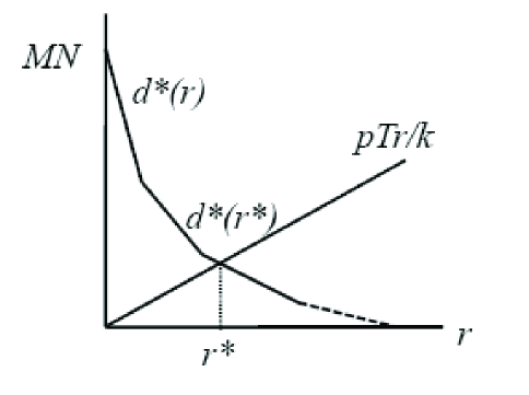
Figure 2: The optimal multiplexing rate $r^{*}$ to balance source and channel distortion.

It should be noted that the tightness of the above bounds only hold when $T\geq M+N-1$. For $T<M+N-1$ the upper bound remains the same while the lower bound changes, which leaves a gap between our bounds.

IV-B Asymptotic Distortion Properties

The asymptotic distortion and optimal distortion exponent from Theorem 1 possess a few non-intuitive properties. First, while it is possible to choose $d^{*}(r)=MN$ (full multiplexing) or $r=\min(M,N)$ (full diversity), it is never optimal to do so. When minimizing $\bar{D}_{\tau}(\mathrm{SNR})$ we require non-zero amounts of both diversity and multiplexing, otherwise one of the terms in the distortion bounds (15) and (18) will not tend to zero as $\mathrm{SNR}$ approaches infinity. It is also interesting to examine the optimal distortion exponent as the block length $T$ or source dimension $k$ become large. As $k$ becomes large (and $T$ remains fixed) we must increase $r^{*}$ in order to match the terms in (20). This is consistent with our intuition since a high dimensional source will require a large amount of multiplexing, otherwise the distortion at the source encoder becomes very large. It is more surprising that as $T$ becomes large (and $k$ remains fixed) we should decrease $r^{*}$, i.e. increase diversity at the expense of multiplexing. This is in contrast to traditional source-channel coding, where we encode our source at a rate just below the channel capacity ($\min(M,N)\log\mathrm{SNR}$) when the block length tends to infinity. In this case, however, we don’t encode at channel capacity because the source dimension $k$ remains fixed as $T$ becomes large. Thus, since the source encoding rate is proportional to $T$, we are already getting an asymptotically large channel rate for source encoding, and therefore should use our antennas for diversity rather than additional rate through multiplexing.

IV-C Source-Channel Code Separation

One feature that we do share with the traditional source-channel coding results is the notion of separation. In a traditional Shannon-theoretic framework, the source encoder needs to know only the channel capacity to design its source code. Then one may encode the source independently of the channel (at the channel capacity rate) and achieve the optimal end-to-end distortion. In this case the end-to-end distortion is due only to the source encoder since the channel is error free (over asymptotically long block lengths).

In our model we consider a source encoder concatenated with a MIMO channel that is restricted to transmission over finite block lengths. With this restriction the channel introduces errors even at transmission rates below capacity. These channel errors give rise to the diversity-multiplexing tradeoff. Under this finite blocklength channel coding we obtain a source and channel coding strategy to minimize end-to-end distortion. Our results indicate that separate source and channel coding is still optimal for this minimization. However, we now get (equal) distortion from both the source and channel code, in contrast to the optimal strategy in Shannon’s separation theorem where the source is encoded at a rate below channel capacity and thus no distortion is introduced by the channel.

IV-D Non-asymptotic Bounds

We now analyze the behavior of our distortion bounds and the corresponding choice of $r^{*}$ for finite $\mathrm{SNR}$. In particular, we will consider the case of large but finite SNR, such that the SNR is sufficiently large to neglect the $O(1)$ term in the exponent of (8) and (18), and to assume $O(1)\approx 1$ and neglect the $o(\log SNR)$ exponential term in (15) and (18). With these approximations the optimal diversity-multiplexing tradeoff is obtained by solving the following convex optimization problem:

$$\min_{r} 2^{-\frac{pT}{k}r\log\mathrm{SNR}}+2^{-d^{*}(r)\log\mathrm{SNR}}$$ (22)

s.t. $$0\leq r\leq\min(M,N).$$

Figures 3, 4, and 5 provide numerical results based on the solution to (22) comparing the total end-to-end distortion versus the number of antennas assigned to multiplexing. Each plot contains four curves that represent different $\mathrm{SNR}$ levels. The difference between the three plots is the ratio of the block length $T$ to source vector dimension $k$. Notice that for $T$ much smaller than $k$ (Figure 3) we will use almost all of our antennas for multiplexing. For $k$ of the same order as $T$ (Figure 4) we will choose about the same number of antennas for multiplexing and for diversity. For $k$ smaller than $T$ (Figure 5) we will use more antennas for diversity than for multiplexing. Note that even at low SNR we can still find $r^{*}$ via the convex optimization formulation in (22), but must include the neglected terms $O(1)$ and $o(\log SNR)$ in the distortion expressions to which we apply this optimization. In our numerical results we found that neglecting these terms for SNRs above 20 dB had little impact.

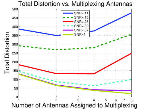
Figure 3: Total distortion vs. number of antennas assigned to multiplexing in an 8x8 system ($T<<k$).

Figure 4: Total distortion vs. number of antennas assigned to multiplexing in an 8x8 system ($T~{}k$).

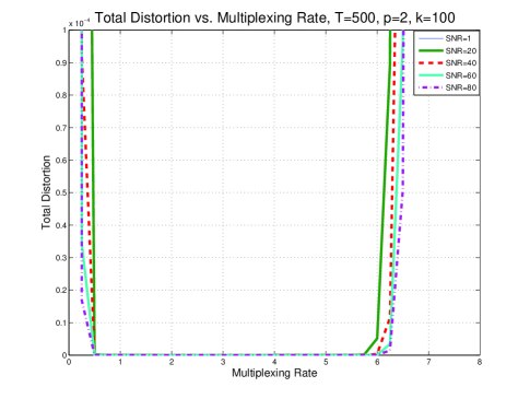
Figure 5: Total distortion vs. number of antennas assigned to multiplexing in an 8x8 system ($T>>k$).

V Practical Source and Channel Coding

While the results in the previous section lead to closed form solutions for optimal joint source-channel coding in the high SNR regime, they only apply to a specific class of source and channel codes and distortion metrics. We now examine the diversity-multiplexing tradeoff for a broad class of source codes, channel codes, and distortion metrics. The basic optimization framework (22) can still be applied to this more general class of problems. Furthermore, this framework can be applied in non-asymptotic settings, thereby allowing us to study the diversity-multiplexing tradeoff under typical operating conditions. In this section we present an example of end-to-end distortion optimization, via the diversity-multiplexing tradeoff, for source/channel distortion models that are fitted to real video streams and MIMO channels.

We use the progressive video encoder model developed in [13]. The overall mean-square distortion is evaluated as

$$D_{\tau}=D_{e}+D_{c},$$ (23)

where $D_{e}$ is the distortion induced by the source encoder and $D_{c}$ is the distortion created by errors in the channel. Although the total distortion is represented by two separate components, each component shares some common terms so we will still have a tradeoff between diversity and multiplexing. The model for source distortion $D_{e}$ developed in [13] consists of a six-parameter analytical formula that is fitted to a particular traffic stream. Numerical results for $D_{e}$ as a function of the source encoding rate are provided in [13, Figure 2]. The source encoder design is based on a parameter $\beta$ corresponding to the amount of redundant data in consecutive encoding blocks. In general a larger value of $\beta$ leads to a smaller $D_{e}$ at the cost of increased complexity.

The model for the channel distortion $D_{c}$ is fitted to the following equation,

$$D_{c}=\sigma^{2}P_{e}(N_{u})\left[\frac{\gamma+\beta}{\gamma}\ln\left(1+\frac{\gamma}{\beta}\right)-\frac{1}{\gamma}+\frac{1}{2}\right],$$ (24)

where given $\beta$ the parameters $\sigma^{2}$ and $\gamma$ are based on the particular source encoder and traffic stream, $N_{u}$ is the number of antennas used for multiplexing, and $P_{e}(N_{u})$ is the probability of codeword error as a function of $N_{u}$. We will assume sources with $\beta=.01$ in our analysis since it provides the lowest distortion for any given rate. This source encoder setting also provides the highest sensitivity to channel errors, which allows us to highlight the tradeoff between multiplexing and diversity in our optimization.

Our channel transmission scheme follows the setup in [16]. We use 8 transmit and 8 receive antennas with a set of linear space-time codes that can trade off multiplexing for diversity (specifically, these codes only trade integer values of $r$ and $(M,N)$). The actual code construction in [16] is fairly complex and involves several inner and outer codes designed to handle both Ricean and Rayleigh fading channels in a MIMO orthogonal frequency division multiplexing (OFDM) system. For the purposes of our numerical results the actual code design is irrelevant, we only require the probability of error as a function of SNR and the number of antennas assigned to multiplexing, which is given in [16, Figure 4]. Our optimization can be applied to space-time channel codes developed by other authors [8, 6, 18] by using the error probability associated with their codes in our optimization.

Since the channel coding scheme of [16] does not permit us to assign fractions of antennas, we must solve the following integer program for the optimal distortion and number of multiplexing antennas:

$$\min_{N_{u}} D_{e}+D_{c}$$ (25)

$$s.t. N_{u}\in\{1,2,4,8\}.$$

Figure 6 contains a set of curves that show the total distortion achieved as a function of the number of antennas assigned to multiplexing. The uppermost curve corresponds to the lowest $\mathrm{SNR}$ and the bottom curve corresponds to the highest $\mathrm{SNR}$. We see that we have an explicit tradeoff here that depends on $\mathrm{SNR}$. At low $\mathrm{SNR}$ the total distortion is minimized by assigning most antennas to diversity to compensate for the high error probability in the channel. As $\mathrm{SNR}$ increases we assign more antennas to multiplexing since this is a better use of antennas when the error probability is low. One significant difference between this plot and the asymptotic results in Section IV is that here we do assign our antennas to full multiplexing as the $\mathrm{SNR}$ becomes large. The reason we observe this behavior is that the rate of our codebook in this example does not scale with $\mathrm{SNR}$. Thus, as the $\mathrm{SNR}$ becomes large we eventually reach a point where distortion would be reduced by moving to a higher rate code that is not available in the 8x8 space-time code under consideration. Hence, the optimal choice in this case is to eventually move to full multiplexing. The implication of this result is that a MIMO system should have enough antennas to exploit full multiplexing at all available $\mathrm{SNR}$s. A design framework for such codes has been developed in [6], but the error probability analysis of these codes is still needed to perform the joint source-channel coding optimization.

Figure 6: Total distortion vs. number of antennas assigned to multiplexing for differing levels of SIR.

VI The Diversity-Multiplexing-Delay Tradeoff

Instead of accepting decoding errors in the channel, many wireless systems perform error correction via some form of ARQ. In particular, the receiver has some form of error detection code, and if a transmission error is detected on a given packet, a feedback path is used to send this error information back to the transmitter, which then resends part or all of the packet to increase the chance of successful decoding. The packet retransmissions, combined with random arrival times of the messages at the transmitter, cause queues to form in front of the source coder and hence each block of data will experience random delays. Here, the notion of delay we wish to capture is the time between the arrival time of a message at the transmitter and the time at which it is successfully decoded at the receiver (also known as the “sojourn time” in queueing systems).

While ARQ increases the probability of decoding a packet correctly, it also introduces additional delay. The window size of the ARQ protocol determines how many retransmission attempts will be made for a given packet. The larger this window size, the more likely the packet will be successfully received, and the larger the possible delays associated with retransmission will be. ARQ can be viewed as a form of diversity, and hence it complements antenna diversity in MIMO systems. For MIMO systems with ARQ, there is a three-dimensional tradeoff between diversity due to multiple antennas and ARQ, multiplexing, and delay. This three-dimensional tradeoff region was recently characterized by El Gamal, Caire, and Damen in [7], and we will use this region in lieu of the Zheng/Tse diversity-multiplexing region in this section. We will first summarize results from [7] characterizing this region, then use this region to optimize the diversity-multiplexing-ARQ tradeoff for distortion under delay constraints.

VI-A The ARQ Protocol and its Diversity Gain

We assume the same $M$x$N$ channel model (2) as before and the following ARQ scheme. Each information message is encoded into a sequence of $L$ blocks each of size $T$. Transmission commences with the first block and after decoding the message the receiver sends a positive (ACK) or negative (NACK) acknowledgement back to the transmitter. In the case of a NACK the transmitter sends the next block in the sequence and the receiver uses all accumulated blocks to try to decode the message. This process proceeds until either the receiver correctly decodes the message or until all $L$ blocks have been sent. If a NACK is sent after the transmission of the $L$th block then an error is declared, the message is removed from the system, and the transmitter starts over with the next queued message. As in [7] we will use the term “round” to describe a single block transmission of length $T$. We will refer to all $L$ rounds associated with the ARQ protocol as an “ARQ block”. Hence, each ARQ block consists of up to $L$ rounds, and each round is of size $T$.

The fading coefficients $h_{ij}$ that model the gain from transmit antenna $i$ to receive antenna $j$ are i.i.d. complex Gaussian with unit variance. The channel gain matrix $\mathbf{H}$ with elements $H(i,j)=(h_{ij}:i\in\{1,\ldots N\},j\in\{1,\ldots,M\})$ is assumed to be known at the receiver and unknown at the transmitter. There are two channel models investigated in [7]: the long-term static model and the short-term static model. In the long-term static model the channel remains constant over each ARQ block of up to $LT$ symbols, and the fading associated with each ARQ block is i.i.d. In the short-term static model the fading is constant over one ARQ round, then changes to a new i.i.d. value. The long-term model applies to a quasi-static situation such as might be seen in a wireless LAN channel. The short-term model is more dynamic and might correspond to fading associated with a portable mobile device. The ARQ diversity gain is very similar for the two models. In particular, the diversity exponent for the short-term static model is a factor of $L$ larger than for the long-term static model, corresponding to the $L$-fold time diversity in the short-term model. We will use the long-term static model in our analysis and numerical results, since it allows us to focus on the diversity associated with the ARQ rather than time diversity. Our analysis easily extends to the short-term static model by adding the extra factor of $L$ to the ARQ diversity exponent.

Under the long-term static channel model, in round $l\in\{1,\ldots,L\}$ of an ARQ block we can represent the channel as

$$\mathbf{Y_{l}}=\sqrt{\frac{\mbox{SNR}}{M}}\mathbf{HX_{l}}+\mathbf{W},$$ (26)

where $\mathbf{X_{l}}\in\mathcal{C}^{M\mathrm{x}T}$ and $\mathbf{Y_{l}}\in\mathcal{C}^{N\mathrm{x}T}$ are the transmitted and received signals in block $l$, respectively. The additive noise vector $\mathbf{W}$ is i.i.d. complex Gaussian with unit variance.

With the above model in hand let us define a family of codes $\{C(\mbox{SNR})\}$, indexed by the SNR level. Each code has length $LT$ and the bit rate of the first block in each code is $b(\mbox{SNR})/T$. Suppose we consider a sequence of ARQ blocks. At time $s$ the random variable $B[s]=b(\mbox{SNR})$ if a message is successfully decoded at the receiver, and $B[s]=0$ otherwise. Then, we can define the average throughput of the ARQ protocol using these codes as

$$\eta(SNR)=\liminf_{\tau\rightarrow\infty}\frac{1}{T\tau}\sum_{s=1}^{\tau}B[s],$$ (27)

and we can view $\eta(\mbox{SNR})$ as the average number of transmitted bits per channel use. Further define $P_{e}(\mbox{SNR})$ as the average probability of error of the ARQ block (i.e. the probability that a NACK is sent after $L$ transmission rounds). The multiplexing gain of the ARQ protocol is defined in [7] as

$$r=\lim_{\mbox{SNR}\rightarrow\infty}\frac{\eta(\mbox{SNR})}{\log\mbox{SNR}},$$ (28)

and the diversity gain as

$$d=-\lim_{\mbox{SNR}\rightarrow\infty}\frac{\log P_{e}(\mbox{SNR})}{\log\mbox{SNR}}.$$ (29)

For each $r$ and $L$ we define the optimal diversity gain $d^{*}(r,L)$ as the supremum of the diversity gain achieved by any scheme. For $L=1$ (i.e. no ARQ) we have the original diversity-multiplexing tradeoff from Section II. Hence, $d^{*}(r,1)$ is the piecewise linear function $d^{*}(r)$ joining the points $(k,(M-k)(N-k)$, at integer values of $k$ for $0\leq k\leq\min(M,N)$. For $L>1$ we have the following result from [7].

Diversity Gain of ARQ: The diversity gain for the ARQ protocol with a maximum of $L$ blocks is

$$d^{*}(r,L)=d^{*}\left(\frac{r}{L}\right).$$ (30)

The diversity gain achieved by ARQ is quite remarkable. According to (30), for any $r<\min(M,N)$ we can achieve the full diversity gain $d=MN$ for sufficiently large $L$. Thus, for $L$ sufficiently large, there is no reason to utilize spatial diversity since all needed diversity can be obtained through ARQ. For $L$ not sufficiently large, the maximum ARQ window size would still be utilized to minimize the amount of spatial diversity required. The diversity-multiplexing-ARQ tradeoff (30) is analogous to the Zheng-Tse diversity-multiplexing tradeoff $d^{*}(r)$. Thus, the same analysis as in Section III can be applied to minimize end-to-end distortion based on the diversity-multiplexing tradeoff $d^{*}(r,L)$ induced by the ARQ. In particular, end-to-end distortion for MIMO channels with asymptotically high SNR and ARQ retransmissions, in the absence of a delay constraint, is minimized using the following procedure:

1. choose the largest ARQ window size $L$ possible,

2. determine the resulting ARQ diversity gain $d^{*}(r,L)$ from (30)

3. solve (20) for the optimal rate $r^{*}$ using $d^{*}(r,L)$ instead of $d^{*}(r)$.

This procedure not only minimizes end-to-end distortion, but also indicates that separate source and channel coding is optimal, provided the source and channel encoders know $r^{*}$ and the maximum value of $L$. Moreover, the results in [8] show that the rate penalty for ARQ is negligible in the high SNR regime.

In order to analyze the diversity, multiplexing, and delay tradeoff for delay-sensitive sources we must recognize two important subtleties about the above results. First, in systems that transmit delay-constrained traffic we may not be able to tolerate a long ARQ window (in some cases ARQ may not be tolerated at all). Second, we must carefully consider the impact of asymptotically high SNR, which is crucial in the proofs of the above results. Specifically, in the high SNR regime the occurrence of a NACK in the ARQ protocol becomes a rare event (i.e. the probability of a NACK tends to zero as SNR approaches infinity). Therefore, with probability tending to one, each message is decoded correctly during the first transmission attempt – resulting in a multiplexing gain equivalent to that of a system without ARQ. The increasingly rare errors are corrected by the ARQ process, which results in increased diversity.

The main difficulty in using these asymptotic results to evaluate delay performance is that in the high SNR regime there is essentially no delay due to ARQ. In other words, queuing delays associated with retransmissions are rare in the high SNR regime. Based on this fact and using standard results from queuing theory, one can show that under stable arrival rates the arriving messages almost always find the system empty. Hence, with high probability an arriving message will immediately begin transmission and suffer no queuing delay. In wireless systems, errors during a transmission attempt are not rare events. Indeed, most wireless systems typically become reliable only after the application of ARQ. In other words, errors after completion of the ARQ process might be rare events, but errors during the ARQ process are not rare. As we shall see in the next subsection, this subtle difference requires a an optimization framework that can model and optimize over the queuing dynamics associated with ARQ.

VI-B Delay-Distortion Model

This section presents our model for a delay-sensitive system. We do not assume a high SNR regime in our analysis since, as stated in the previous section, this leads to rare ARQ errors and hence effectively removes the ARQ queuing delay. We do assume that the finite SNR is fixed for each problem instance, i.e. we do not optimize power control, although this optimization was investigated in [7] and shown to provide significant diversity gains in the long-term static channel.

We assume the original source data $u$ is a random vector with probability density $h(u)$, which has support on a closed, bounded subset of $\Re^{k}$ with non-empty interior. During each transmission block of length $T$ an instance of $u$ arrives at the system independently with probability $\lambda$ and is queued for transmission. We assume that each message has a deadline $k$ at the receiver. Hence, if a message arrives at time $t$ and is not received by time $t+kT$ then its deadline expires and the message is dropped from the system. We assume that each message is quantized according to the scheme discussed below. The quantized version of each message is then mapped into a codeword in the codebook $\{C(\mbox{SNR})\}$ and passed to the MIMO-ARQ transmitter discussed in the previous section.

Due to the random message arrival times and the random completion times of the ARQ process we will have queuing and delay in this system. Our goal is to select a diversity gain, multiplexing gain, and ARQ window size to minimize the distortion created by both the quantizer and the messages lost due to channel error or delay. The intuition behind the diversity-multiplexing-ARQ tradeoff is straightforward. We would like to use as much multiplexing as possible since this will allow us to use more bits to describe a message and reduce encoder distortion. However, high levels of multiplexing induce more errors in the wireless channel, thereby requiring longer ARQ windows to reduce errors. The longer ARQ windows induce higher delays, which also cause higher distortion due to messages missing their deadlines. We must balance all of these quantities to optimize system performance.

We use the same vector encoder and distortion model from Section III. As before, we assume that the total average distortion $D_{\tau}(F,\mbox{SNR})$ can be split into two dependent pieces

$$D_{\tau}(F,SNR)=D_{s}(F)+D_{e}(d,\mbox{SNR}),$$ (31)

where $D_{e}(d,\mbox{SNR})$ is the distortion caused by messages declared in error. Here the errors are incurred whenever the ARQ process fails or when a message’s deadline expires. We also assume the distortion due to erroneous messages is bounded by the overall loss probability:

$$D_{e}(d,\mbox{SNR})\leq P_{e}(\mbox{SNR})+P\{Delay>k\},$$ (32)

where $P\{Delay>k\}$ is the probability that a message violates its deadline and $P_{e}(\mbox{SNR})$ is the probability of error for the ARQ block, which depends on its window size $L$.

Our goal is to minimize the total delay-distortion bound

$$D_{\tau}(F,\mbox{SNR})\leq D_{s}(F)+P_{e}(\mbox{SNR})+P\{Delay>k\}.$$ (33)

In order to optimize (33) we require a formulation that accounts for the different delays experienced by each message. Hence, as described in the next section, we turn to the theory of Markov decision processes to model and solve this problem.

VI-C Minimizing Distortion via Dynamic Programming

We now develop a dynamic programming optimization framework to minimize (33). We assume without loss of generality that the queue in our system is of maximum size $k$. This is not a restrictive assumption since each message requires at least one time block of size $T$ for transmission, hence any arriving message that sees more than $k$ messages in the queue will not be able to meet its deadline and could be dropped without affecting our performance analysis. Note that unlike standard queuing models that only track the number of messages awaiting transmission, we must also track the amount of time a particular message has waited in the queue. In particular, given that one message is queued for transmission our state space model must differentiate between a message that has just arrived and a message whose deadline is about to expire. Since the queue size is bounded, we can only have a finite number of messages in the queue, and hence the combined message and waiting time model exists in a finite space.

We define the queue process $X_{Q}=(X_{Q}(n):n\geq 0)$, which takes values on a finite space $\mathcal{X_{Q}}$. Similarly, we define the state of the ARQ process $X_{L}=(X_{L}(n):n\geq 0)$ on a finite space $\mathcal{X_{L}}$. Here, the state of the ARQ process denotes the number of the current transmission round in the current ARQ block. Finally, we define the overall state of the system as a process $X=(X(n):n\geq 0)$ such that $X(n)=(X_{Q}(n),X_{L}(n))$ (i.e. the space $\mathcal{X}$ is the product space of $\mathcal{X_{Q}}$ and $\mathcal{X_{L}}$).

Since the arrival process is geometric and each ARQ round is assumed to be i.i.d., the process $X$ is a finite-state discrete-time Markov chain. The transition dynamics of this Markov chain are governed by the choices of diversity, multiplexing, and the ARQ window size. We assume that at the start of each ARQ block the transmitter chooses the number of bits to assign to the vector encoder and hence the amount of spatial diversity and multiplexing in the codeword selected from $\{C(\mbox{SNR})\}$. The transmitter also selects the length of the ARQ window. These choices then remain fixed until either the message is received or the ARQ window expires. Define the space of actions $\mathcal{A}$ as the set of all possible combinations of multiplexing gain and ARQ window length. Note that a choice of multiplexing gain implicitly selects the number of bits given to the source encoder as well as the amount of spatial diversity. We assume that the number of antennas $M$ and $N$ are finite and that the ARQ window size is also finite. Hence, the action space $\mathcal{A}$ is a finite set.

We define the control policy $g$ as a probability distribution on the space $\mathcal{X}\;\mathrm{x}\;\mathcal{A}$. We can view the elements of $g$ as

$$g(x,a)=P\{\mathrm{action}\;a\;\mathrm{chosen}\;\mathrm{in}\;\mathrm{state}\;x\},\;\forall x\in\mathcal{X}\;,a\in\mathcal{A}.$$

For any control $g$, the Markov chain $X$ is irreducible and aperiodic. Define $Q(g)$ as the transition matrix for $X$ corresponding to control policy $g$. Hence, $Q(g)=(Q_{i,j}(g):i,j\in\mathcal{X})$ is a stochastic matrix with entries

$$Q_{i,j}(g)=P\left(X(n+1)=j|X(n)=i,g\right)$$

$$= \sum_{a\in\mathcal{A}}P\left(X(n+1)=j|X(n)=i,A(n)=a)g(i,a)\right).$$

For each state-action pair we define a reward function $r(x,a)$. For the states in $\mathcal{X}$ corresponding to completion of the ARQ process the reward function denotes the distortion incurred in that particular state. Hence,

$$r(x,a)=2^{-ps/k}+I[\mathrm{ARQ}\;\;\mathrm{Fails}]+I[Delay>k].$$

Let $\mathcal{G}$ be the set of all available control policies. Then for any $g\in\mathcal{G}$ define the limiting average value of $g$ starting from state $x$ as

$$V(x,g) = \limsup_{n\to\infty}\left[\left(\frac{1}{n+1}\right)\sum_{k=0}^{n}E_{x,g}\left[r(X(k),g)\right]\right],$$

where $r(X(k),g)$ is the random reward earned at time $k$ under control policy $g$. Since $X$ is an irreducible and aperiodic Markov chain for any control $g$ we know from [2] that the above value function reduces to

$$V(x,g)=\pi(g)r(g)\;\forall\;x\in\mathcal{X},$$ (34)

where $\pi(g)=\pi(g)Q(g)$ is the stationary distribution of $X$ under control $g$ and $r(g)$ is the column vector of rewards earned for each state $x\in\mathcal{X}$ under control $g$. Hence, the value function is simply the expected value of our reward function $r$ with respect to the stationary distribution of $X$. Notice that given our definition for $r$ in (VI-C), the value function $V(g)$ provides us with the delay-based distortion (33) caused by control policy $g$. Thus we want to minimize distortion by minimizing the value function $V(g)$.

Specifically, our goal is to find a $g\in\mathcal{G}$ that minimizes $V(x,g)$. From [2] we know this problem can be solved through the following linear program.

$$\min_{s}\sum_{x\in\mathcal{X}}\sum_{a\in\mathcal{A}}r(x,a)s_{xa}$$ (35)

subject to:

$$\sum_{x\in\mathcal{X}}\sum_{a\in\mathcal{A}}\left(\delta(x,x\,^{\prime})-p(x\,^{\prime}|x,a)\right)s_{xa} = 0,\;x\,^{\prime}\in\mathcal{X}$$

$$\sum_{x\in\mathcal{X}}\sum_{a\in\mathcal{A}}s_{xa} = 1,$$

$$s_{xa}\geq 0;\;a\in\mathcal{A},\;x\in\mathcal{X},$$

where $\delta(x,x\,^{\prime})$ is the Kronecker delta, $s_{xa}$ is the steady-state probability of being in state $x$ and taking action $a$, and $p(x\,^{\prime}|x,a)$ is the probability of jumping to state $x\,^{\prime}$ given action $a$ in state $x$. The state-action frequencies $s_{xa}$ provide a unique mapping to an optimal control ${g}^{*}$ [2].

With this dynamic programming formulation in hand we can solve for the optimal diversity gain, multiplexing gain, and ARQ window size as a function of queue state and deadline sensitivity. We demonstrate the performance of these solutions with a numerical example in the next subsection.

VI-D Distortion Results

Consider the ARQ system described above with messages arriving in each time block with probability $\lambda=0.9$. We assume a 4x4 MIMO-ARQ system ($M=N=4$) with an SNR of 10 dB that utilizes the incremental redundancy codes proposed in [6], which have been shown to achieve the diversity-multiplexing-ARQ tradeoff. For these codes we allow the ARQ window size to take values in a finite set $L\in\{1,\ldots,4\}$. We also consider the deadline length $k$ ranging over several values ($k\in\{2,\ldots,8\}$) to examine the impact of delay sensitivity on the solution to our dynamic program (35). For each value of $k$ we solve a new version of (35). The plots below contain the data accumulated by averaging over all of these solutions.

Figure 7 plots the optimal ARQ window length as a function of queue state for different values of $k$. We see that for short deadlines we cannot afford long ARQ windows for any queue state. As the deadlines become more relaxed we can increase the ARQ window size. However as the queue fills up we are forced to again decrease the amount of ARQ diversity.

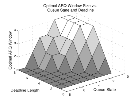
Figure 7: Optimal ARQ window size vs. queue state vs. deadline length $k$ (SNR=10 dB).

Figure 8 plots the optimal multiplexing gain $r$ as a function of queue state for different values of $k$. Here we see that with short deadlines we must use fairly low amounts of spatial multiplexing (i.e. high spatial diversity), since we cannot use ARQ diversity. As the deadlines become more relaxed we can increase the amount of spatial multiplexing and use ARQ for diversity. Once again, as the queue fills up we must switch back to low levels of multiplexing or, equivalently, high levels of diversity to ensure a lower error probability and hence that fewer retransmissions are needed to clear a given message from the system.

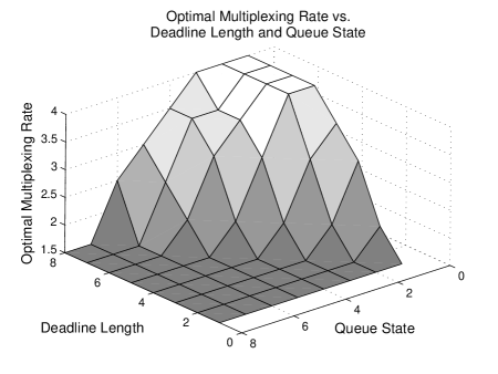
Figure 8: Optimal multiplexing gain vs. queue state vs. deadline length $k$ (SNR=10 dB).

We also evaluate the performance advantage gained by adapting the settings of diversity, multiplexing, and ARQ rather than choosing fixed allocations. For $k=4$ we computed the distortion resulting from all possible fixed allocations of ARQ window length and multiplexing gain. The curved surface in Figure 9 plots the distortion of these fixed allocations for all values of $L$ and $r$. The flat surface in Figure 9 is the distortion achieved by the adaptive scheme (plotted as a reference), which indicates a distortion reduction of up to 70 dB. Even in the most favorable cases, the adaptive scheme outperforms any fixed scheme by more than 50%.

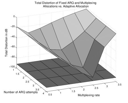
Figure 9: Distortion for the fixed allocation problem vs. multiplexing gain vs. ARQ window size (SNR=10 dB).

VII Summary

We have investigated the optimal tradeoff between diversity, multiplexing, and delay in MIMO systems to minimize end-to-end distortion under both asymptotic assumptions as well as in practical operating conditions. We first considered the tradeoff between diversity and multiplexing without a delay constraint. In particular, for the asymptotic regime of high SNR and source dimension, we obtained a closed-form expression for the optimal rate on the Zheng/Tse diversity-multiplexing tradeoff region as a simple function of the source dimension, code blocklength, and distortion norm. We also showed that in this asymptotic regime separate source and channel coding at the optimized rate minimizes end-to-end distortion. However, in contrast to codes designed according to Shannon’s separation theorem, the finite blocklength assumption in our setting causes distortion to be introduced by both the source code and the channel code, even though the source encoding rate is below channel capacity. We showed that the same optimization framework can be applied even without an asymptotically large SNR. However, outside this asymptotic regime, closed-form expressions for the optimal diversity-multiplexing tradeoff (and corresponding transmission rate) cannot be found, and convex optimization tools are required to find this optimal operating point. Finally, we developed an optimization framework to minimize end-to-end distortion for a broad class of practical source and channel codes, and applied this framework to a specific example of a video source code and space-time channel code. Our numerical results illustrate quantitatively how the optimal number of antennas used for multiplexing increases with both the source rate and the SNR.

We then extended our analysis to delay-constrained sources and MIMO systems using an ARQ retransmission protocol. ARQ provides additional diversity in the system at the expense of delay. Minimizing end-to-end delay thus entails finding the optimal operating point on the diversity-multiplexing-delay tradeoff region. We developed a dynamic programming formulation for this optimization to capture the diversity-multiplexing tradeoffs of the channel as well as the dynamics of random message arrival times and random ARQ block completion times. The dynamic program can be solved using standard techniques, which we applied to a 4x4 MIMO system with different ARQ window sizes and delay constraints. We obtained numerical results indicating the optimal amount of diversity, multiplexing, and ARQ to use as a function of the queue state and message deadline. We also demonstrated that adaptation of the diversity-multiplexing characteristics of the MIMO channel code to the time-varying backlog in the system leads to distortion reduction of up to 70 dB versus a static allocation.

The unconsummated union between information theory and networks has vexed both communities for many years. As pointed out in [10], part of the reason for this disconnect is that source burstiness and end-to-end delay are major components in the study of networks, yet play little role in traditional Shannon theory where delay is asymptotically infinite and channel capacity inherently assumes a source with infinite data to send. We hope that our work provides one small step towards consummating this union by merging information-theoretic tradeoffs associated with the channel with models and analysis tools from networking to handle source burstiness and system delay. Much work remains to be done in this area by extending our ideas and developing new ones for coupling the fundamental performance limits of general multihop networks with queuing delay, traffic statistics, and end-to-end metric optimization for heterogeneous applications running over these networks.

VIII Acknowledgments

We are deeply grateful to the four reviewers for their detailed and insightful comments, which helped to greatly improve the clarity and exposition of the paper. We want to thank Reviewer D in particular for suggesting Figure 2 to illustrate the optimization of the multiplexing rate $r^{*}$.

List of Figures and Captions

• Figure 1: The optimal diversity-multiplexing tradeoff for $T\geq M+N-1$

• Figure 2: The optimal multiplexing rate $r^{*}$ to balance source and channel distortion

• Figure 3: Total distortion vs. number of antennas assigned to multiplexing in an 8x8 system ($T<<k$)

• Figure 4: Total distortion vs. number of antennas assigned to multiplexing in an 8x8 system ($T~{}k$)

• Figure 5: Total distortion vs. number of antennas assigned to multiplexing in an 8x8 system ($T>>k$)

• Figure 6: Total distortion vs. number of antennas assigned to multiplexing for differing levels of SIR.

• Figure 7: Optimal ARQ window size vs. queue state vs. deadline length $k$ (SNR=10 dB)

• Figure 8: Optimal multiplexing gain vs. queue state vs. deadline length $k$ (SNR=10 dB)

• Figure 9: Distortion for the fixed allocation problem vs. multiplexing gain vs. ARQ window size (SNR=10 dB)

Author Biographies

Holliday: Tim Holliday received the B.S. degree in general engineering from Harvey Mudd College, Claremont, CA, in 1997; the M.S. degree in electrical engineering from Stanford University, Stanford, CA, in 2001; and the Ph.D. degree in management science and engineering from Stanford University in 2004. His industry experience includes summer internships at Lucent Technologies Bell Labs in summers of 2000 and 2001. He also served as a Communications Officer in the U.S. Air Force Reserve from 1997 through 2004. From 2004-2006 he was a Postdoctoral Research Associate at Princeton University, Princeton, NJ. In 2007 he joined Goldman Sachs as an associate. His research interests include stochastic processes and modeling, cross-layer design in wireless communications, and information theory.

Goldsmith: Andrea J. Goldsmith is a professor of Electrical Engineering at Stanford University, and was previously an assistant professor of Electrical Engineering at Caltech. She has also held industry positions at Maxim Technologies and at AT&T Bell Laboratories, and is currently on leave from Stanford as co-founder and CTO of Quantenna Communications, Inc. Her research includes work on capacity of wireless channels and networks, wireless communication and information theory, energy-constrained wireless communications, wireless communications for distributed control, and cross-layer design of wireless networks. She is author of the book “Wireless Communications” and co-author of the book “MIMO Wireless Communications,” both published by Cambridge University Press. She received the B.S., M.S. and Ph.D. degrees in Electrical Engineering from U.C. Berkeley.

Dr. Goldsmith is a Fellow of the IEEE and of Stanford. She has received several awards for her research, including the National Academy of Engineering Gilbreth Lectureship, the Alfred P. Sloan Fellowship, the Stanford Terman Fellowship, the National Science Foundation CAREER Development Award, and the Office of Naval Research Young Investigator Award. She was also a co-recipient of the 2005 IEEE Communications Society and Information Theory Society joint paper award. She currently serves as associate editor for the IEEE Transactions on Information Theory and as editor for the Journal on Foundations and Trends in Communications and Information Theory and in Networks. She was previously an editor for the IEEE Transactions on Communications and for the IEEE Wireless Communications Magazine, and has served as guest editor for several IEEE journal and magazine special issues. Dr. Goldsmith is active in committees and conference organization for the IEEE Information Theory and Communications Societies and is an elected member of the Board of Governors for both societies. She is a distinguished lecturer for the IEEE Communications Society, the vice-president and student committee founder of the IEEE Information Theory Society, and was the technical program co-chair for the 2007 IEEE International Symposium on Information Theory.

Poor: H. Vincent Poor (S 72, M 77, SM 82, F 87) received the Ph.D. degree in EECS from Princeton University in 1977. From 1977 until 1990, he was on the faculty of the University of Illinois at Urbana-Champaign. Since 1990 he has been on the faculty at Princeton, where he is the Dean of Engineering and Applied Science, and the Michael Henry Strater University Professor of Electrical Engineering. Dr. Poor s research interests are in the areas of stochastic analysis, statistical signal processing and their applications in wireless networks and related fields. Among his publications in these areas are the recent book MIMO Wireless Communications (Cambridge University Press, 2007), co-authored with Ezio Biglieri, et al, and the forthcoming book Quickest Detection (Cambridge University Press, 2008), co-authored with Olympia Hadjiliadis.

Dr. Poor is a member of the National Academy of Engineering, a Fellow of the American Academy of Arts and Sciences, and a former Guggenheim Fellow. He is also a Fellow of the Institute of Mathematical Statistics, the Optical Society of America, and other organizations. In 1990, he served as President of the IEEE Information Theory Society, and in 2004-07 as the Editor-in-Chief of these Transactions. Recent recognition of his work includes the 2005 IEEE Education Medal, the 2007 IEEE Marconi Prize Paper Award, and the 2007 Technical Achievement Award of the IEEE Signal Processing Society.

References

- [1] K. Azarian, H. El Gamal, and P. Schniter, “On the Achievable Diversity-Multiplexing Tradeoff in Half-Duplex Cooperative Channels”, IEEE Trans. Inform. Theory, Vol. 51, No. 12, pp. 4152–4172, Dec. 2005.
- [2] Bertsekas, D. P., Dynamic Programming and Optimal Control, Boston: Athena Scientific, 1995.
- [3] J. Bucklew and G. Wise, “Multidimensional asymptotic quantization theory with th power distortion measures”, IEEE Trans. Inform. Theory, Vol. 28, No. 2, pp. 239 -247, Mar. 1982.
- [4] T. M. Cover and J. A. Thomas, Elements of Information Theory, New York: John Wiley & Sons, 1991.
- [5] I. Csiszár and J. Körner, Information Theory: Coding Theorems for Discrete Memoryless Systems, Academic Press, New York, 1981.
- [6] H. El Gamal, G. Caire, and M. O. Damen, “Lattice coding and decoding achieve the optimal diversity-vs-multiplexing tradeoff of MIMO channels”, IEEE Trans. Inform. Theory , Vol. 50, No. 6, pp. 968–985, June 2004.
- [7] H. El Gamal, G. Caire, and M. O. Damen, “The MIMO ARQ Channel: Diversity-Multiplexing-Delay Tradeoff”, IEEE Trans. Inform. Theory, Vol. 52, No. 8, pp3601–3621, Aug. 2006 .
- [8] H. El Gamal and A. R. Hammons Jr, “On the design of algebraic space-time codes for MIMO block fading channels”, IEEE Trans. Inform. Theory , vol. 49, No. 1, pp. 151–163, Jan. 2003.
- [9] H. El Gamal and M. O. Damen, “Universal space-time coding,” IEEE Trans. Inform. Theory , Vol. 49, No. 5, pp. 1097–1119, May 2003.
- [10] A. Ephremides and B. Hajek, “Information theory and communication networks: an unconsummated union,” IEEE Trans. Inform. Theory , Vol. 44, No. 6, pp. 2416–2434, Oct. 1998.
- [11] A. Gersho, “Asymptotically Optimal Block Quantization”, IEEE Trans. Inform. Theory , Vol. 25, No. 7, pp. 373–380, July 1979.
- [12] A. Gersho and R. M. Gray, Vector Quantization and Signal Compression , Boston: Kluwer Academic, 1992.
- [13] B. Girod, K. Stuhlmuller, N. Farber, “Trade-Off Between Source and Channel Coding for Video Transmission”, Proc. of the IEEE Intl. Conf. Image Proc. (ICIP), Vol. 1, pp. 399–402, Sept. 2000.
- [14] D. Gross and C.M. Harris, Fundamentals of Queueing Theory, New York: John Wiley & Sons, 2000.
- [15] B. Hochwald, K. Zeger, “Tradeoff Between Source and Channel Coding”, IEEE Trans. Inform. Theory, Vol. 43, No. 5, pp. 1412–1424, Sept. 1997.
- [16] M. Kuhn, I. Hammerstroem, A. Wittneben, “Linear Scalable Space-Time Codes: Tradeoff Between Spatial Multiplexing and Transmit Diversity”, Proc. of SPAWC 2003, pp. 21–25, June 2003.
- [17] J.N. Laneman, E. Martinian, G.W. Wornell, J.G. Apostolopoulos, “Source-channel diversity for parallel channels”, IEEE Trans. Inform. Theory. Vol. 51, No. 10, pp. 3518–3539, Oct. 2005.
- [18] H. F. Lu and P. V. Kumar, “Rate-diversity tradeoff of space-time codes with fixed alphabet and optimal constellations for PSK modulationn”, IEEE Trans. Inform. Theory, Vol. 49, No. 10, pp. 2747–2751, Oct. 2003
- [19] J. Max, “Quantizing for Minimum Distortion”, IEEE Trans. Inform. Theory, Vol. 6, No. 1, pp. 7–12, March 1960.
- [20] B.A. Sethuraman, B.S. Rajan, and V. Shashidhar, “Full diversity, high rate, space-time block codes from division algebras,” IEEE Trans. Inform. Theory, Vol. 49, No. 10, pp. 2596–2616, Oct. 2003.
- [21] K. Stuhlmuller, N. Farber, M. Link, and B. Girod, “Analysis of Video Transmission over Lossy Channels’, IEEE J. Select. Areas Commun., Vol. 18, No. 6, pp. 1012–1032, June 2000.
- [22] A. Trushkin, “Sufficient conditions for uniqueness of a locally optimal quantizer for a class of convex error weighting functions,” IEEE Trans. Inform. Theory, Vol. 28, No. 2, pp. 187 -198, Mar. 1982.
- [23] D. Tse, P. Viswanath and L. Zheng “Diversity-Multiplexing Tradeoff in Multiple Access Channels”, IEEE Trans. Inform. Theory, vol. 50, No. 9, pp. 1859-1874, Sept 2004.
- [24] H. Yao and G.W. Wornell, “Achieving the Full MIMO Diversity-Multiplexing Frontier with Rotation-Based Space-Time Codes”, Proc. Allerton Conf. Commun., Contr., and Computing, Oct. 2003.
- [25] P. Zador, “Asymptotic quantization error of continuous signals and the quantization dimension,” IEEE Trans. Inform. Theory, Vol. 28, No. 2, pp. 139 -149, Mar. 1982.
- [26] K. Zeger and V. Manzella, “Asymptotic bounds on optimal noisy channel quantization via random coding,” IEEE Trans. Inform. Theory, Vol. 40, No. 6, pp. 1926- 1938, Nov. 1994.
- [27] L. Zheng, D. Tse, “Diversity and Multiplexing: the Optimal Tradeoff in Multiple Antenna Channels”, IEEE Trans. Inform. Theory , Vol. 49, No. 5, pp. 1073–1096, May 2003.