Faster exact Markovian probability functions for motif occurrences: a DFA-only approach

Abstract

Background: The computation of the statistical properties of motif occurrences has an obviously relevant practical application: for example, patterns that are significantly over- or under-represented in the genome are interesting candidates for biological roles. However, the problem is computationally hard; as a result, virtually all the existing pipelines (for instance [1]) use fast but approximate scoring functions, in spite of the fact that they have been shown to systematically produce incorrect results [2][3]. A few interesting exact approaches are known [2][4], but they are very slow and hence not practical in the case of realistic sequences. Results: We give an exact solution, solely based on deterministic finite-state automata (DFAs), to the problem of finding not only the $p$-value, but the whole relevant part of the Markovian probability distribution function of a motif in a biological sequence. In particular, the time complexity of the algorithm in the most interesting regimes is far better than that of [2], which was the fastest similar exact algorithm known to date; in many cases, even approximate methods are outperformed. Conclusions: DFAs are a standard tool of computer science for the study of patterns, but so far they have been sparingly used in the study of biological motifs. Previous works [2][5] do propose algorithms involving automata, but there they are used respectively as a first step to build a Finite Markov Chain Imbedding (FMCI), or to write a generating function: whereas we only rely on the concept of DFA to perform the calculations. This innovative approach can realistically be used for exact statistical studies of very long genomes and protein sequences, as we illustrate with some examples on the scale of the human genome.

1 Introduction

It is difficult for analysis tools to meet the challenge represented by the ever-increasing data flux coming from high-throughput post-genomics experiments. One sector where this problem is particularly evident is that of sequence analysis.

As it is well known, for example, the detection of statistically relevant nucleotide sequences that occur repeatedly in a (possibly very long) stretch of genetic material has interesting biological aspects. Motifs appearing significantly more or less than mere chance would dictate can hint to the presence of relevant regulatory regions, e.g. promoters or tandem repeats. Statistical properties may relate to structural ones as well: recently, for example, a 117Kb periodicity in E.coli has been linked to topological features of its chromosomes [6]; the exceptional statistics of the “crossover hot spot instigator” close to the genome core common to different strains of E.coli can be possibly be linked to the protection of that part of the chromosome from recombination events [7].

However, it is not easy to pinpoint what statistically relevant exactly means in the context of sequence analysis. In particular, the problem is computationally hard for at least two reasons:

1. given a sequence of symbols taken from an alphabet $\mathcal{A}$ of size $a$, the number of possible sequences of length $L$ is $a^{L}$, that is, the number of possible strings grows exponentially with the length of the considered stretch. It should then not come as a surprise to the reader the fact that, at least in one approach found in the literature, the solution is given in terms of an NP-hard algorithm [4].

2. complicated motifs can overlap in non-trivial ways, making simple statistical approximations unreliable and requiring the exploitation of more sophisticated analytic techniques. As a matter of fact, it has been proved that in many common situations approximate methods do systematically fail to predict correct statistical estimators [2][3]; thus, possessing a fast non-approximate method would seem essential to provide solid and unbiased foundations to characterize under- and over-represented motifs from the point of view of their biological role.

In fact, a good deal of attention has been devoted in the recent past to the problem of detecting DNA motifs which appear with anomalous frequency inside a genome, and this problem has prompted the development of a diverse range of tools and algorithms for the study of the statistics of pattern occurrences [4][8][9]. However, to be computationally feasible most of the proposed methods involve either quite drastic approximations on the statistical model which is used to describe the genome (see for example [1]), or some additional information (e.g., a training set) to be supplied by the user (see for example [10]).

Although very slow in many realistic regimes and as a consequence probably unpractical for everyday use, a few algorithms to compute exact probability distribution functions for motif occurrences are known. We distinguish two main methods: the first one, based on position-weighted matrices, is presented in [4]; the second one, introduced in [2], takes advantage of Finite Markov Chain Imbeddings (FMCIs) using Deterministic Finite-state Automata (DFAs) to deduce the Markovian transition matrix of the model.

In this paper we introduce a third exact method. The general statistical setup is similar to that of the latter method (we take as null hypothesis the fact that our sequence is generated by a Markov model of arbitrary order), but the proposed algorithm is very different. In particular, we show that:

1. contrarily to what all the recent literature about exactly solved Markov models would seem to imply, FMCIs are completely inessential to evaluate the probability distribution functions of motifs.

2. a simpler approach entirely based on DFAs is possible. The simpler resulting algorithm naturally lends itself to a much better optimization, making the exact analysis of genomes of realistic size feasible. In fact, in many regimes the obtained performance is even better than that of the approximate large-deviations and Gaussian models of [3] (see Table 2).

As an application, we produce in Section 5 an analysis of various motifs in the human X chromosome ($L\sim 1.5\cdot 10^{8}$), and of more than 16.000 transcription-factor binding sites in S.cerevisiae ($L\sim 1.2\cdot 10^{7}$). Both cases are out of reach for exact FMCI methods (see Table 2).

1.1 Background about exact Markovian methods

Defining $L$ as the length of the sequence under analysis, $N_{\operatorname{obs}}$ as the number of observed occurrences of the examined motif $\mathfrak{m}$, $a$ as the number of symbols in the alphabet $\mathcal{A}$, and $s$ as the number of states of a DFA which is able to recognize and count the motif $\mathfrak{m}$ (see Section 2.1), the exact algorithm presented in [2] to compute the $p$-value of $\mathfrak{m}$ for a Markov model of order $m$ runs in a time proportional to

$$\mathcal{O}\left(a\times s\times\left(N_{\operatorname{obs}}+1\right)\times L\right).$$ (1)

It is not immediate to get a practical comprehension of the meaning of such an expression, so we briefly analyze it here. We can distinguish two main relevant asymptotic regimes: the short-pattern regime, and the long-pattern regime.

In the short-pattern regime, the cost of the algorithm turns out to be essentially quadratic in the length $L$ of the considered sequence. In fact, in the case of $m=0$ and uniform probability distribution of symbols the typical recorded number of observed pattern occurrences may be estimated as

$$N_{\operatorname{obs}}\sim\frac{L}{a^{\ell}},$$ (2)

being $\ell$ the length of the pattern; similar results hold for more complicated Markov models. Inserting this estimate into (1), one immediately realizes that in this regime the cost becomes proportional to $L^{2}$.

On the other hand, for long patterns the cost is linear in $L$; in fact —as suggested by (2) again— the typical occurrence numbers in this case are $N_{\operatorname{obs}}=0$ or $N_{\operatorname{obs}}=1$, so the cost becomes essentially independent of $N_{\operatorname{obs}}$ and proportional to $L$.

Of course, being the size of realistic biological sequences very large (for example, in the range $10^{7}$-$10^{10}$ for the case of a typical genome) an algorithm which is linear, or —even worse— quadratic in $L$ is essentially unpractical: both the long- and the short-pattern regimes will be unaccessible to it.

1.2 Results and discussion

In this paper we show how a formulation of motif counting in terms of systolic DFAs (see Section 2.2) allows us to directly deduce an algorithm with cost $\mathcal{O}\left(a\times s\times\left(N_{\operatorname{obs}}+1\right)\times L\right)$, that is, equivalent in complexity to that presented in [2]. Furthermore, additional formal developments described in Section 2.3 make it possible to write the probability distribution function $p\!\left(x\right)$ of the occurrences of a motif $\mathfrak{m}$ as

$$p\!\left(x\right)=\operatorname{Tr}\!\left(\left(\mathcal{M}\!\left(x\right)\right)^{L}\cdot v_{0}\right),$$ (3)

where, as explained in Section 2.3, $v_{0}$ is an $\mathbbm{R}$-valued vector of length $s$; in turn, $\mathcal{M}\!\left(x\right)$ is an $s\times s$ sparse square matrix with $a\times s$ non-zero elements, each of its elements being a polynomial in $x$ of degree $\leqslant N_{\operatorname{obs}}^{\max}=L/s$ (see Section 2.3). Of course, through their construction $\mathcal{M}$ and $v_{0}$ depend parametrically both on the order $m$ of the Markov model and on the pattern $\mathfrak{m}$ being examined; however, for the sake of notational simplicity we will not indicate this fact explicitly in the rest of the paper, as much as we will often drop the dependence of $\mathcal{M}$ on $x$ as well.

There are two main possible evaluation strategies for such an expression:

1. we compute $p\!\left(x\right)$ as

   $$p\!\left(x\right)=\mathcal{M}\cdot\left(\mathcal{M}\cdot\left(\ldots\cdot\left(\mathcal{M}\cdot v_{0}\right)\ldots\right)\right);$$

   we are able to take advantage of the sparsity of the matrix $\mathcal{M}$, but the resulting algorithm has a final complexity of

   $$\mathcal{O}\!\left(a\times s\times\left(N_{\operatorname{obs}}+1\right)^{2}\times L\right),$$

   being thus slower than the FMCI method in [2] due essentially to the quadratic cost of polynomial multiplication of matrix elements.

2. we compute $\mathcal{M}^{L}$ directly by logarithmic decomposition, and its product with the initial condition vector $v_{0}$ in the end. The naive cost of such a scheme is now

   $$\mathcal{O}\!\left(s^{3}\times\left(N_{\operatorname{obs}}+1\right)^{2}\times\log L\right),$$

   which is much less than (1) in the linear long-pattern regime.

   In addition, in Section 3 we observe that it is possible to use the FFT algorithm to perform polynomial multiplication as a convolution of the coefficients; as a result, the whole bulk of $p\!\left(x\right)$ may be obtained with a complexity of

   $$\mathcal{O}\!\left(s^{2}\times\log L\times L\right)$$ (4)

   which is much faster than that of the algorithm of [2] in the quadratic short-pattern regime. In addition, defining $p_{\varepsilon}\!\!\left(x\right)$ as the truncated distribution obtained from $p\!\left(x\right)$ by suppressing the tail regions as long as $p\!\left(x\right)<\varepsilon\max p$, and introducing the quantity

   $$\operatorname{base}_{\varepsilon}\!\!\left(p\right):=\operatorname{length}\!\left(\operatorname{supp}p_{\varepsilon}\right),$$ (5)

   a successive refinement of the method allows to obtain for this technique an even better final cost of

   $$\mathcal{O}\!\left(s^{3}\times\operatorname{base}_{\varepsilon}\!\!\left(p\right)\times\log L\right),$$ (6)

   which is excellent in the case of the evaluation of both the linear and the quadratic regime, given that $\operatorname{base}_{\varepsilon}\!\!\left(p\right)\ll L$ in all practical cases (see Table 2).

To illustrate the quality of the results just obtained we consider two examples from real-life situations in the case of a Markov model of order $1$:

1. a very long sequence (i.e. the entire human genome, $\sim 3\cdot 10^{9}$ base pairs) and a long pattern of length $16$, such that $N_{\operatorname{obs}}=1$. In this case, one can deduce from (6) that the complexity speedup obtained by our algorithm w.r.t. the FMCI-based one would be $\sim 2\cdot 10^{5}$.

2. an entire human chromosome ($\sim 1.5\cdot 10^{8}$ base pairs) and a very short pattern, ATC for example; this is the nastiest possible case for the exact algorithm of [2], since it falls in its quadratic regime. Here our algorithm outperforms the FMCI one by a factor of $\sim 5\cdot 10^{6}$.

In fact, Equation (6) tells us that the performance of our exact technique is quite close to that of the approximate Gaussian method described in [3] (which is essentially proportional to $s\times\log L$); maybe more surprisingly, in the most interesting regime of moderate $m$, long sequences and not too short patterns our method is in general even faster than both the large-deviations and the Gaussian approximations, and possibly much faster (see Table 2 below). In addition, when thinking about these comparisons it should not be forgotten that —unlike approximate methods— our faster scheme is still able to produce the whole bulk of the probability distribution, from which all the interesting statistical quantities can be straightforwardly computed. A more complete comparison of the existing Markov methods to ours is presented in Section 5, together with a discussion of the timings and the results obtained for some test examples.

2 System and methods

It is very easy to write a computer program which, given a stretch of DNA or protein of length $L$, finds all the contained sub-patterns of any length $\ell$ together with the corresponding frequencies. As mentioned before, however, supposing that a given motif has been found $N_{\operatorname{obs}}$ times it is not easy to define and compute what the expected occurrence probability $p\!\left(N_{\operatorname{obs}}\right)$ should be: i.e., it is not easy to guess whether the measured number $N_{\operatorname{obs}}$ is a priori large or small.

In fact, a satisfactory and very well-known conceptual framework to tackle similar problems has been formulated decades ago in the context of computer science, where the ability of recognizing (“parsing”) symbol strings in programs is essential; it is based on deterministic finite-state automata (DFA for shortness). Such theoretical devices are ubiquitous and fundamental in computer science, so we will not describe their principles here; we just mention that the interested reader may easily find many thorough introductions to the field in standard computer-science literature — one classic reference for this subject being for example [11].

What makes DFAs particularly interesting from the point of view of biological analysis is that they can naturally be linked to Markov models of sequences. In fact, we can formulate the Markovian null hypothesis that our stretch of DNA or protein is completely determined by its statistics of order $m$, i.e. by the frequency of appearance of each unique sub-string of length $m+1$ (with $m\geqslant 0$) contained in the sequence; in this case, if we apply to the string being examined a sliding window of length $m+1$, we can straightforwardly reinterpret the stretch as a sequence of consecutive transitions between groups of $m+1$ symbols, and link the Markov chain statistics to the probability for the DFA to make a transition from a state to another one.

This remarkable fact has been realized only recently in the context of the analysis of biological sequences [2]; however, although leading to the relatively fast FMCI-based algorithm mentioned before, the approach presented in [2] uses DFAs just as auxiliary tools to produce the transition matrix between states of the underlying Markov process.

In the present article we show how the statistical description of a sequence in terms of pure DFAs is worthwhile by itself, and may lead to much faster numerical evaluation schemes. To make the reader more at ease, throughout the following sections we will illustrate the formal developments of our technique by means of a worked example in the case of statistics of order 0.

2.1 A case study

Let us consider a stretch of genome with $L=10$ in which the motif ATC appears two times. To decide if this frequency means that ATC is for some reason overrepresented, given some Markovian statistics we must compute the probability that such a pattern can appear randomly two times in a genome stretch of length $10$, and compare it to the observed probability of the event. More in general, how to calculate the probability of ATC to appear $n$ times?

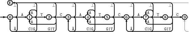
Figure 1: An infinite DFA able to recognize and count all occurrences of motif ATC. When the automaton is in states 0, 1 or 2 the pattern has occurred exactly 0 times; when the automaton is in states 3, 4 or 5 the pattern has occurred 1 times; and so on. State E is the end-of-input.

Of course, one could try to give an answer in terms of direct enumeration. In fact, this approach works quite well for very short sequences; however, the reader can easily convince themselves that the method is both very expensive and very difficult to generalize algorithmically as the length $L$ of the sequence increases, and it becomes completely unpractical for the analysis of genomes of realistic size (i.e., $L\sim 10^{7}$-$10^{9}$ bases).

To answer the question in more general terms, we begin by writing down the DFA of Figure 1.

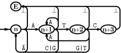
Figure 2: The basic building block of Figure 1. The complete automaton is obtained by replicating this block as many times as the number of observed occurrences, plus one.

Such a DFA is obtained by chaining three identical basic blocks as that represented in Figure 2, each one matching one occurrence of the original ATC motif. Starting from state 0, the automaton works by reading in one character at the time from the stretch of genome, and changing its internal state step by step according to the input; for example, the automaton of Figure 1 when processing the string CAATCGTCATCG will run through the states 0, 1, 1, 2, 3, 3, 3, 3, 4, 5, 6, 6. The meaning of the states is thus as follows: when the automaton is in state 0, it is waiting to read the first A; in state 1, it is waiting for a T after having read one or more As; in state 3, exactly one ATC has been read, possibly preceded by any string different from ATC and followed by any number of bases different from A; in state 6, exactly two ATCs have been read, preceded and separated by any possible string different from ATC, and followed by any string which is not a substring of ATC; and likewise for any other state (the special character$\boldsymbol{\perp}$meaning the end of input, so that state E is the final one, reached after all the input string has been consumed by the automaton). We observe that the construction of the automaton is far from being trivial; however, as emphasized before standard algorithms to solve the problem are known since a long time and may easily be found in the literature [11]. Chaining more than one basic block as in Figure 1 allows us to count the number of instances of ATC found in the genome: by construction, when processing any of the genomes which contain exactly two occurrences of pattern ATC the automaton will always end up in states 6, $\boldsymbol{7}$ or $\boldsymbol{8}$.

So far, we have thus succeeded in restating our original problem: all the genomes we are interested in (e.g. those containing two instances of pattern ATC) are the genomes that make the automaton of Figure 1 terminate by reaching state E through states 6, $\boldsymbol{7}$ or $\boldsymbol{8}$. How to extract direct numerical information out of this statement? There are basically two answers to this question.

The first answer is that by the method of generating functions one can work out analytically the probability for the automaton to be in state 6, 7 or 8 (and in all other states as well) after having read any arbitrary input; again, introductory examples to this computational procedure may be found in [12]. This method is appealing since it allows the computation of the probability distribution function in closed form, but it suffers from an obvious important drawback: for a sequence of length $L$ it requires a Taylor expansion of order $L$; given that the typical size of a relatively short bacterial genome is already in the range of $10^{6}$-$10^{7}$ bases, one would expect this technique to be unpractical when analyzing realistic stretches of genome. Although this is indeed the case, it is worthwhile to note that the method has nonetheless been exploited successfully in the context of biological research for the case of shorter genomes [5]; this result may serve as a useful reference.

2.2 The systolic DFA

We observe that a second approach is possible, which is simpler, easier to implement and more amenable to direct interpretation and fast numerical evaluation. Quite surprisingly, to the best of the authors’ knowledge this powerful method does not seem to have been proposed before for any relevant practical application, neither in computer science nor in biology.

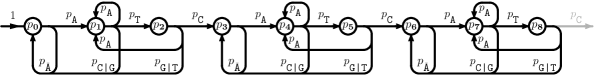
Figure 3: The automaton of Figure 1 reinterpreted as a systolic array. Transitions to the end-of-input state E have been omitted.

To implement it, we turn the DFA of Figure 1 into a systolic array, which is a weighted graph where the propagation of flow from node to node happens proportionally to the transition probabilities, and at a constant speed of one edge per alphabet symbol read by the automaton in the sequence; such a construction owes its name to the fact that it can be assimilated to an hydraulic circuit where the probability $1$ enters from the left at time $0$, and is then split and pumped at constant speed towards the following states of the automata, reaching more and more nodes as time goes by.

For example, let us suppose to start at time $0$ —that is, at sequence length $L=0$— with all the probability in state 0. Since state 0 has two outgoing connections, one to state $\boldsymbol{1}$ and one to itself, at time $1$ (or, equivalently, at length $L=1$) the content of state 0 will have been pumped partly into state 1 and partly back to state 0; in particular, state 1 will now contain $p_{\text{{{1}}}}\!\left(t=1\right)=p_{\text{{{0}}}}\!\left(t=0\right)\cdot p_{\text{{{A}}}}=1\cdot p_{\text{{{A}}}}=p_{\text{{{A}}}}$, and $p_{\text{{{0}}}}\!\left(t=1\right)$ will be the new content of state 0, that is $p_{\text{{{0}}}}\!\left(t=0\right)\cdot p_{\overline{\text{{{A}}}}}=p_{\overline{\text{{{A}}}}}$. The idea can easily be generalized to later times (i.e. longer sequences) if the structure of the automaton is taken into due account.

By construction, at any given time (or sequence length $L$) the probability distribution $p(n)$ as a function of the number of pattern occurrences $n$ may thus be obtained just by adding the contents of the states three by three: for example, if $L=10$ then $p(0)=p_{\boldsymbol{0}}\!\left(t=10\right)+p_{\boldsymbol{1}}\!\left(t=10\right)+p_{\boldsymbol{2}}\!\left(t=10\right)$, $p(1)=p_{\boldsymbol{3}}\!\left(10\right)+p_{\boldsymbol{4}}\!\left(10\right)+p_{\boldsymbol{5}}\!\left(10\right)$, and so on (the extension to automata with different number of states is obvious); this direct interpretation should not be overlooked, since it is fundamental for the developments to come. We note that the probability flows and redistributes from node to node as a consequence of time evolution but its total amount is not consumed in the process; in fact, the sum of the weights of the outgoing connections for each node is by definition $1$, being it also the sum of the transition probabilities over all possible symbols. The automaton of Figure 1 re-interpreted as a systolic array is shown in Figure 3, and its evolution up to $t=512$ (that is, up to $L=512$) is listed in Table 1

$L$	$p_{\boldsymbol{0}}$	$p_{\boldsymbol{1}}$	$p_{\boldsymbol{2}}$	$p_{\boldsymbol{3}}$	$p_{\boldsymbol{4}}$	$p_{\boldsymbol{5}}$	$p_{\boldsymbol{6}}$	$p_{\boldsymbol{7}}$	$p_{\boldsymbol{8}}$	$L$	$p_{\boldsymbol{0}}+p_{\boldsymbol{1}}+p_{\boldsymbol{2}}$	$p_{\boldsymbol{3}}+p_{\boldsymbol{4}}+p_{\boldsymbol{5}}$	$p_{\boldsymbol{6}}+p_{\boldsymbol{7}}+p_{\boldsymbol{8}}$
0	$1$	$0$	0	0	0	0	0	0	0	16	$\sim 0.797$	$\sim 0.188$	$\sim 0.0148$
1	$\frac{3}{4}$	$\frac{1}{4}$	0	0	0	0	0	0	0	32	$\sim 0.614$	$\sim 0.312$	$\sim 0.0661$
2	$\frac{11}{16}$	$\frac{1}{4}$	$\frac{1}{16}$	0	0	0	0	0	0	64	$\sim 0.365$	$\sim 0.383$	$\sim 0.185$
3	$\frac{43}{64}$	$\frac{1}{4}$	$\frac{1}{16}$	$\frac{1}{64}$	0	0	0	0	0	128	$\sim 0.129$	$\sim 0.275$	$\sim 0.282$
…										256	$\sim 0.0160$	$\sim 0.0691$	$\sim 0.146$
8	$\frac{40531}{65536}$	$\frac{3379}{16384}$	$\frac{3841}{65536}$	$\frac{2221}{32768}$	$\frac{157}{8192}$	$\frac{127}{32768}$	$\frac{83}{65536}$	$\frac{3}{16384}$	$\frac{1}{65536}$	512	$\sim 0.000249$	$\sim 0.00215$	$\sim 0.00922$

Table 1: Flow of probability propagating through the systolic array of Figure 3, as the array consumes longer and longer stretches of genome. To compute this table we chose $p_{\text{{{A}}}}=p_{\text{{{C}}}}=p_{\text{{{G}}}}=p_{\text{{{T}}}}=0.25$. Apart from the probability of recording zero patterns, which always decreases exponentially after a transient phase (see Section 2.3), the other probabilities show a bell-shaped behaviour w.r.t. genome length: the probability of recording exactly $N_{\operatorname{obs}}$ patterns grows, peaks for a certain length of the genome stretch, and decreases afterwards. It should be noted that starting from $L>8$ the probabilities add up to a number which is smaller and smaller than $1$, since more and more probability flux is transmitted to states $p_{\boldsymbol{9}},p_{\boldsymbol{1}\boldsymbol{0}},\ldots$ .

.

The interesting point about such a construction is that it is able to keep track of the effects of all possible input sequences at the same time by superposition, as a consequence of the fact that the probability present in a node at time $t$ splits over all possible transitions at time $t+1$. Basically, we have turned our original automaton, which was a simple recognizer, into a much more powerful device, which can now compute the probability of being in each state after having read all possible inputs; it should thus not come as a surprise the statement that we are now able to scan in polynomial time sets of strings whose cardinality grows exponentially with the length of the sequence.

We note that even a naive interpretation of this setup immediately yields a viable computational scheme.

Algorithm 1

(Systolic Naive). Given a Markov model of order $m$ and a motif $\mathfrak{m}$, compute $p\!\left(x\right)$ as follows:

1. generate the systolic automaton associated to $\mathfrak{m}$ by the given Markov model; in particular, set a suitable initial condition $p_{\boldsymbol{i}}\!\left(t=0\right)$ for the states $(1\leqslant i\leqslant s)$

2. for $t=1$ to $L$ do

   • evaluate the systolic propagation in the automaton:

     for $i=1$ to $s$ do

     • $p_{\boldsymbol{i}}\!\left(t\right)=0$

     done

     foreach connection from state $\boldsymbol{s}_{\operatorname{source}}^{k}$ to state $\boldsymbol{s}_{\operatorname{sink}}^{k}$ with weight $w_{k}$ $(1\leqslant k\leqslant a\times s)$ do

     • $p_{\boldsymbol{s}_{\operatorname{sink}}^{k}}\!\!\left(t\right)=p_{\boldsymbol{s}_{\operatorname{sink}}^{k}}\!\!\left(t\right)+w_{k}\cdot p_{\boldsymbol{s}_{\operatorname{source}}^{k}}\!\!\left(t-1\right)$

     done

   done

3. return the probability distribution function as $\displaystyle p\!\left(x\right)=\sum_{n=x\cdot s}^{\left(x+1\right)\cdot s-1}p_{\boldsymbol{n}}\!\left(L\right),\;\;\forall x\in\left[0,N_{\operatorname{obs}}^{\max}\right]$. $\Box$

This algorithm possesses at least two very desirable properties:

1. apart from possible small roundoff errors in the evaluation of Markovian statistics, it is exact and numerically stable.

2. it allows the optimized evaluation of $p\!\left(x\right)$ in the region $x\in\left[0,N_{\operatorname{obs}}^{\max}\right]$; in fact, this effect may be obtained just by truncating the automaton after $\left(N_{\operatorname{obs}}+1\right)$ basic blocks, and letting the probability flux which should go to higher stages simply disperse.

Considering that each state of the automaton has $a$ possible outgoing transitions, the computational cost of the algorithm in the latter truncated case can readily be written as $\mathcal{O}\!\left(a\times s\times L\times\left(N_{\operatorname{obs}}+1\right)\right)$, which by a striking coincidence turns out to be exactly the same as that of the very different FMCI-based exact algorithm presented in [2]. We also point out that taking advantage of the cutoff technique which will be explained in Section 3 we could slightly improve on this result by discarding the tail of very small elements coming ahead of the distribution.

2.3 Further developments

In fact, much better results may be obtained; to proceed, however, we have to develop a slightly more elaborate description of the problem.

First of all, we observe that it is not really necessary to have in the automaton as many building blocks as the largest number of pattern occurrences $N_{\operatorname{obs}}^{\max}=L/s$ which might appear in a sequence; in fact, it is possible to get a “folded” version of the automaton just by adding one single connection to its basic block. For example, the reader may easily convince themselves that the automaton of Figure 4

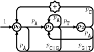
Figure 4: The folded version of the systolic array of Figure 3. The transition from state $\boldsymbol{2}$ to state $\boldsymbol{0}$ is a counting one, as indicated by the “+” symbol. Transitions to the end-of-input state have been omitted.

is entirely equivalent to that of Figure 3, provided that we supply a mechanism to keep track of the fact that the probability flux associated to a number $N$ of motif occurrences in state $\boldsymbol{2}$ becomes associated to $N+1$ occurrences when passing to state $\boldsymbol{0}$ through the special connection indicated by the “$+$” symbol; that is why we name such a link a counting transition. We will describe in a moment one possible way to implement a bookkeeping mechanism like the one just mentioned. We also note that our treatment introduces a slight but significant difference w.r.t. the related approach presented in [13]: in fact, as from the standard theory of DFA construction one finds in the latter work a final counting state instead of our counting transition, resulting in our automaton being one state shorter; although we will not examine further this issue in the present paper, it is possible that our slightly more compact construction could indeed be used to improve some of the results obtained in [13].

Secondly, it is worthwhile to cast the problem in matrix form. To this end, we observe that it is possible to express the systolic propagation of the probability flux in terms of a transition matrix $\mathcal{M}$, which describes the modification in the content of the states of the automaton as the computation proceeds from time $t$ to time $t+1$ (that is, from the length $L$ of the sequence read so far by the automaton to length $L+1$). This goal may be obtained quite straightforwardly just by arranging as a matrix the transition probabilities from one state to another.

In particular, if there were not any mechanism in place to record the number of observed patterns, $\mathcal{M}$ could be defined quite simply as an $s\times s$ matrix of the form

$$\mathcal{M}_{ij}:=p\!\left(\boldsymbol{i}\rightarrow\boldsymbol{j}\right).$$

For example, for the automaton in figure 4 one would write

$$\mathcal{M}_{0}=\left(\begin{array}[]{ccc}p_{\overline{\text{{{A}}}}}&p_{\text{{{C|G}}}}&p_{\text{{{C}}}}+p_{\text{{{G|T}}}}\\ p_{\text{{{A}}}}&p_{\text{{{A}}}}&p_{\text{{{A}}}}\\ 0&p_{\text{{{T}}}}&0\end{array}\right),$$ (7)

the columns representing (in order) the state which the automaton leaves on reception of a new symbol and the rows being indexed by the state reached by the automaton: at the intersection between any column and any row one would find the probability of such a transition to happen. Note that by definition all the columns would be normalized to 1.

We have only elucidated half of the matrix structure so far, though: our finite automata has a special counting transition, which allows us to remember, in any state, how many times the motif has been observed. A convenient way to represent this feature is by replacing the content of each state of the automaton with a polynomial: the coefficient of order $k$ of the polynomial will then represent the probability that the motif has been observed $k$ times. Accordingly to this convention, the elements of the transition matrix need to be replaced by a polynomial as well; in particular, one has to multiply the probability of the counting transition(s) by $x$, since their effect is to increase by one the number of motifs met so far.

For example, assuming all the probabilities to be $p_{\text{{{A}}}}=p_{\text{{{C}}}}=p_{\text{{{G}}}}=p_{\text{{{T}}}}=0.25$ the complete counting transition matrix for the automaton of figure 4 will now be

$$\mathcal{M}\!\left(x\right)=\left(\begin{array}[]{ccc}0.75&0.50&0.5+0.25x\\ 0.25&0.25&0.25\\ 0&0.25&0\end{array}\right),$$ (8)

the only difference w.r.t. the non-counting matrix $\mathcal{M}_{0}$ of (7) lying in the transition probability from state 2 to state 0, which now has been replaced by $p_{\text{{{G|T}}}}+p_{\text{{{C}}}}x$.

To complete the formalism, one just needs to describe how the probability flux is distributed among the states of the automaton at the beginning of the computation; this can be done by simply letting the product of matrices operate on a real-valued vector $v_{0}$ of length $s$ which expresses the initial condition. The probabilities of being in any particular state can thus be deduced by multiplying the matrix $\mathcal{M}$ by itself $L$ times and applying the result to $v_{0}$; in the end, the elements of the obtained vector must be summed over, since we are not interested any longer in how the probability is distributed among the states of the automaton. The resulting polynomial will then correspond to our probability distribution. This way, we get to the final formula, Equation (3).

The reader may easily verify that a repeated application of the matrix appearing in Equation (8) to the initial condition defined by

$$v_{0}=\left(\begin{array}[]{c}1\\ 0\\ \vdots\\ 0\end{array}\right)$$

indeed reproduces Table 1. In particular, all the construction carried out in this Section can be directly extended to the cases of generic pattern and of Markov model of generic order by supplying the correct automaton with its initial condition to the matrix formalism just described (this fact is used in [13] as well); indeed, different choices for the model or $\mathfrak{m}$ only modify the actual contents of $\mathcal{M}$ and $v_{0}$ in Equation (3), which remains correct.

This way of restating the original problem elicits very interesting considerations. For example:

1. $p_{\boldsymbol{0}}$ always decreases exponentially after a transient

2. more stringent conclusions may be drawn about the unimodality of $p\!\left(x\right)$

3. the causality requirement to the propagation of probability flux imposes specific constraints to the form of the transition matrix; such property might possibly be used to speed up the computation of $p\!\left(x\right)$ even more.

In general, although in the present paper we will not pursue any formal investigation, we emphasize that Equation (3) indeed is a perfect place where a rigorous study of the statistical properties of Markovian probability distribution functions can be started.

Finally, it is straightforward to obtain the naive costs of the different possible strategies to evaluate Equation (3); we recall that such results have already been presented in Section 1.2.

3 Algorithm

Everything is now in place to describe our algorithm for the fast evaluation of probability distribution functions of Markov models.

The key observation to obtain an algorithm with superior performance w.r.t. that presented in [2] is to note that multiplication of polynomials may be better performed in terms of a convolution of their coefficients.

Algorithm 2

(Polynomial multiplication by Discrete Fourier Transformation). Given two polynomials $p\!\left(x\right)$ and $q\!\left(x\right)$, compute $pq\!\left(x\right)$ as follows:

1. extend $p\!\left(x\right)$ and $q\!\left(x\right)$ to two polynomials $p^{\prime}\!\left(x\right)$ and $q^{\prime}\!\left(x\right)$ of degree $d^{\prime}=\deg\!\left(p\right)+\deg\!\left(q\right)$ by zero padding.

2. define and compute $\mathfrak{F}\!\left(pq)\right.$ as $\mathfrak{F}\!\left(pq\right)_{i}:=\mathfrak{F}\!\left(p^{\prime}\right)_{i}\mathfrak{F}\!\left(q^{\prime}\right)_{i}$, $0\leqslant i\leqslant d^{\prime}$.

3. return the polynomial product as $pq\!\left(x\right)=\mathfrak{F}^{-1}\!\left(\mathfrak{F}\!\left(pq\right)\right)$. $\Box$

Of course, the main point of interest for our application is that the naive evaluation of $pq\!\left(x\right)$ entails $\left(\deg\!\left(p\right)+1\right)\times\left(\deg\!\left(q\right)+1\right)$ operations, while the use of Algorithm 2 coupled to Fast Fourier Transform (FFT) would require only $\mathcal{O}\!\left(\deg pq\times\log\!\left(\deg pq\right)\right)$ operations to perform the same computation, making the behaviour switch from quadratic to linear. We observe that in the literature it is not easy to find direct applications of this scheme, possibly due to its sensitivity to numerical noise which will be analyzed in more detail below; however, the algorithm is indeed applied in indirect form in some cases, for example when computing products of modulo polynomials (as in the so called Karatsuba multiplication [14]).

Let us note that if we consider polynomial-valued matrices the following relation holds:

$$\mathcal{M}\cdot\mathcal{N}=\mathfrak{F}^{-1}\!\left(\mathfrak{F}\!\left(\mathcal{M}\right)\cdot\mathfrak{F}\!\left(\mathcal{N}\right)\right)$$

where by definition

$$\left(\mathfrak{F}\!\left(\mathcal{M}\right)\right)_{ij}:=\mathfrak{F}\!\left(\mathcal{M}_{ij}\!\left(x\right)\right);$$

this means that the Fourier operator applied to polynomial coefficients commutes with matrix multiplication.

A natural and appealing idea is then to use an FFT setup to directly compute the power $\mathcal{M}^{L}$ of our polynomial-valued matrix appearing in (3). Nonetheless, two objections should be addressed.

First of all, as from Algorithm 2 a (technical) problem when using the FFT algorithm in the context of polynomial multiplication is that care must be taken to ensure that FFT vectors are larger than the degree of the resulting polynomial, otherwise overlaps will occur. This issue increases the memory requirement of the algorithm by a factor of two, but otherwise it has no relevant effect on the evaluation strategy for $p\!\left(x\right)$.

A much more delicate issue is that the FFT algorithm is very sensitive to the noise introduced by rounding errors; in particular, if our bell-shaped distribution is to be represented as a (long) polynomial obtained by repeated multiplications of shorter ones, the typical condition number of the coefficients will be large, while the FFT algorithm can be faithful only to the coefficients whose magnitude does not differ from that of the largest coefficient for more than the numerical precision of the floating-point type used; this shall have the effect of making unreliable the computation of the smaller coefficients of the polynomial — that is, the computation of the tails of the distribution and hence of the $p$-value. However, it is easy to answer this objection, at least when the proposed algorithm is used to compute biologically relevant quantities. In detail:

1. occurrences of motifs observed in practical situations only very rarely fall in the far tails of the distribution (and in any case, we can always quantify algorithmically when our computed $p$-value becomes unreliable).

2. even if the computation of the tails becomes unreliable, the FFT algorithm is still perfectly able to deduce all the relevant statistical quantities of the distibution —which only depend on the bulk of the distribution, not on the exact knowledge of its tails— and hence the $z$-value, which is probably even more significant and informative than the $p$-value in the case of a very unlikely occurrence number.

We can now formulate without concerns an effective strategy to evaluate $\mathcal{M}^{L}$ in Equation (3), and thus the bulk of $p\!\left(x\right)$, by an FFT-based technique.

Algorithm 3

(Systolic Fast via FFT). Given a Markov model of order $m$ and a motif $\mathfrak{m}$, compute $p\!\left(x\right)$ as follows:

1. generate the systolic automaton associated to $\mathfrak{m}$ by the given model.

2. deduce from the systolic automaton the transition matrix $\mathcal{M}$ and the initial condition $v_{0}$.

3. create the two auxiliary square matrices power and result of size $s$.

4. initialize: $\text{{{power}}}\leftarrow\mathfrak{F}\!\left(\mathcal{M}\right)$, $\text{{{result}}}\leftarrow\mathfrak{F}\!\left(\operatorname{identity}_{s}\right)$, $N\leftarrow L$.

5. compute $\mathfrak{F}\!\left(\mathcal{M}^{L}\right)$ by binary decomposition in power as:
   while true do

   • as necessary, apply a cutoff function to the elements of power and result:

     $\text{{{power}}}\leftarrow\operatorname{cutoff}\left(\text{{{power}}}\right)$, $\text{{{result}}}\leftarrow\operatorname{cutoff}\left(\text{{{result}}}\right)$;

     if $N\operatorname{mod}2=1$ then

     • $\text{{{result}}}\leftarrow\text{{{result}}}\,\cdot\,\text{{{power}}};$

     $N\leftarrow\left\lfloor N/2\right\rfloor$;

     if $N=0$ then

     • break;

     $\text{{{power}}}\leftarrow\text{{{power}}}\,\cdot\,\text{{{power}}}$

   done.

6. return the probability distribution function as $\operatorname{Tr}\!\left(\mathfrak{F}^{-1}\!\left(\text{{{result}}}\right)\cdot v_{0}\right)$. $\Box$

We will explain soon how the cutoff function appearing at point (5) should be chosen; for the moment, let us pretend that it is the identity. In this case, recalling that $N^{\max}_{\operatorname{obs}}=L/s$ by construction of the (systolic) automaton, the cost of the algorithm is given by

$$\mathcal{O}\!\left(3\times s^{2}\times\left(N_{\operatorname{obs}}^{\max}+1\right)\times\log\!\left(N^{\max}_{\operatorname{obs}}+1\right)+2\times s^{3}\times\left(N_{\operatorname{obs}}^{\max}+1\right)\times\log L\right)=\mathcal{O}\!\left(s^{2}\times L\times\log L\right),$$

which is Equation (4); the first term in the l.h.s. comes from the Fourier transformations of $\mathcal{M}$, $\operatorname{identity}_{s}$ and result, while the second one —which is dominant if no cutoff is applied— is due to the $2\times\log L$ matrix multiplications occurring in the algorithm.

It is worthwhile to note that, although already excellent from the point of view of performance (in particular w.r.t. the complexity of the FMCI algorithm [2] in the quadratic short-pattern regime, as already pointed out in Section 1.2) this scheme can be further improved by an appropriate choice of the function $\operatorname{\mathit{cutoff}}$ which appears in Algorithm 3.

In fact, we have already pointed out before that our knowledge of $p\!\left(x\right)$ as obtained from an FFT-based algorithm is naturally limited by the numerical precision $\varepsilon:=10^{-d}$ of our floating-point type, $d$ being the number of available decimal digits; as anticipated in Section 1.2, it is then natural to introduce a truncated distribution function $p_{\varepsilon}\!\!\left(x\right)$, which is obtained from $p\!\left(x\right)$ by removing its tails both on the left and the right extrema, in the region (if any) where their value falls below the threshold given by $\varepsilon\max p$. As argued before, $p_{\varepsilon}\!\!\left(x\right)$ keeps all the information which are needed to compute the statistical indicators we are interested in, and furthermore the truncation process does not introduce numerical instabilities; however, this choice of the cutoff has two contrasting implications on the complexity of the algorithm.

The first one is that the cutoffing step slows down the computation; in fact, both the matrices power and result appearing in Algorithm 3 store their elements in Fourier space, and as a result one needs to Fourier transform back and forth at each application of the cutoff. On the other hand, the second consequence is that after having applied the cutoff we need less polynomial coefficients than $N_{\operatorname{obs}}^{\max}+1=L/s+1$ to represent each element of $\mathcal{M}\!\left(x\right)$, since the tails where the distribution is small have now been eliminated; this fact turns out to be a relevant advantage in terms of computational efficiency in many cases, winning in particular a factor which is typically very big in the large-$L$ regime, and thus justifying this choice of the cutoff.

Defining $\operatorname{base}_{\varepsilon}$ as in Equation (5), we can then compute the final complexity of this new algorithm as

$$\mathcal{O}\!\left(s^{2}\times\operatorname{base}_{\varepsilon}\!\!\left(p\right)\times\log\operatorname{base}_{\varepsilon}\!\!\left(p\right)\times\left(3+4\times\log L\right)+2\times s^{3}\times\operatorname{base}_{\varepsilon}\!\!\left(p\right)\times\log L\right)$$

$$= \mathcal{O}\!\left(s^{2}\times\operatorname{base}_{\varepsilon}\!\!\left(p\right)\times\log L\times\left(2\times s+4\times\log\operatorname{base}_{\varepsilon}\!\!\left(p\right)\right)\right)$$

from which Equation (6) immediately follows; depending on $s$ the dominant term is usually the first one (which comes from the $4\times\log L$ FFTs taking place during the evaluation of the $\operatorname{cutoff}$ function), but in some practical cases it could be as well the second one (which comes from matrix multiplications). We note that this result is tipically —that is, for moderate values of $s$ w.r.t. $L$— much better than that of Equation (4); so, the formula just obtained justifies the claim of Section 1.2. Another virtue of such a choice for the $\operatorname{cutoff}$ function is that it lowers the memory requirements of the algorithm, bringing them from $\mathcal{O}\!\left(2\times s^{2}\times L/s\right)=\mathcal{O}\!\left(s\times L\right)$ to the usually much smaller

$$\mathcal{O}\!\left(s^{2}\times\operatorname{base}_{\varepsilon}\!\!\left(p\right)\right).$$ (9)

A remarkable feature of this computational scheme is that it is able to automatically lock itself onto the relevant part of the distribution function, leaving the tails off; no parameters need to be specified except for the cutoff, which in turn can be automatically determined with some simple heuristics from the numerical precision of the floating-point type used.

Finally, we emphasize that cutting off the support is the only natural choice for an FFT algorithm, given again what has been described above about the sensitivity of the FFT to numerical noise; in particular, it is not possible to evaluate $p\!\left(x\right)$ partially, truncating it at $N_{\operatorname{obs}}$ as it is done in [2] or in Section 2.2. On the other hand, the final cost (6) is to be understood as the cost to obtain the whole bulk of $p\!\left(x\right)$, while the much higher cost (1) of [2] is the cost of obtaining only the part of $p\!\left(x\right)$ ranging from $0$ to $N_{\operatorname{obs}}$.

4 Implementation

All the considerations carried out in the last Sections have been gathered and implemented in a computer program called PATRONUS (from “PATtern Recognition by Optimized Numerical Universal Scoring”). The program is mostly written in Objective Caml [15], a very-high-level functional programming language, with some C insets: the part of the code which computes the power $\mathcal{M}^{L}$ of the transition operator for the systolic DFA through Algorithm 3 (see Section 3) is critical for the overall performance of the program since most of the total execution time is spent there; thus, the relative code has been optimized at low level using C, and packaged as an OCaml primitive. This architecture allows to get the best from both worlds (the superior formal power of OCaml, and the numerical efficiency of C) at the expense of only some minor performance penalty.

For the FFT-related code we used FFTW [16], a C library which is both very portable and carefully optimized, and offers sophisticated routines which transparently take advantage of vector SIMD extended instructions on the processors where they are present.

$m=1$
Genome	$L$	$\mathfrak{m}$	$N_{\operatorname{obs}}\!\!\left(\mathfrak{m}\right)$	$\operatorname{base}_{\varepsilon}\!\!\left(p\right)$	spatt	PATRONUS	ldspatt	gpatt
HIV1	9181		108	153	0.20s	0.084s	0.012s	0.004s
B.subtilis	4214630		50985	3480	$\infty$	1.1s	0.32s	0.12s
S.cerevisiae	12156678	CCT	138318	5913	$\infty$	1.6s	0.90s	0.34s
Human X Chr.	151058754		2512286	24456	$\infty$	6.3s	11s	4.2s
B.subtilis	4214630		1919	613	$\infty$	0.62s	0.47s	0.12s
S.cerevisiae	12156678	ATATTC	7054	1178	$\infty$	0.85s	1.3s	0.34s
Human X Chr.	151058754		61408	3601	$\infty$	2.9s	17s	4.2s
B.subtilis	4214630		52	73	64s	0.26s	0.49s	0.12s
S.cerevisiae	12156678	ATATTCATA	173	181	$\infty$	0.43s	1.4s	0.34s
Human X Chr.	151058754		2146	544	$\infty$	1.1s	17s	4.2s
B.subtilis	4214630		2	14	4.5s	0.28s	0.47s	0.12s
S.cerevisiae	12156678	ATATTCATATTC	9	24	41s	0.30s	1.3s	0.34s
Human X Chr.	151058754		44	66	$\infty$	0.42s	16s	4.2s
		AATATTCATATTC	10	37	$\infty$	0.42s	17s	4.2s
Human X Chr.	151058754	TAATATTCATATTC	3	20	260s	0.68s	16s	4.2s
		ATAATATTCATATTC	1	13	130s	0.48s	17s	4.2s
$m=2$
Genome	$L$	$\mathfrak{m}$	$N_{\operatorname{obs}}\!\!\left(\mathfrak{m}\right)$	$\operatorname{base}_{\varepsilon}\!\!\left(p\right)$	spatt	PATRONUS	ldspatt	gpatt
B.subtilis	4214630		52	104	110s	1.4s	0.50s	0.12s
S.cerevisiae	12156678	ATATTCATA	173	216	$\infty$	1.9s	1.4s	0.34s
Human X Chr.	151058754		2146	673	$\infty$	5.3s	16s	4.2s
B.subtilis	4214630		2	18	7.2s	1.0s	0.49s	0.12s
S.cerevisiae	12156678	ATATTCATATTC	9	30	68s	1.1s	1.3s	0.34s
Human X Chr.	151058754		44	94	$\infty$	1.7s	17s	4.2s
		AATATTCATATTC	10	49	$\infty$	1.6s	17s	4.2s
Human X Chr.	151058754	TAATATTCATATTC	3	24	350s	1.5s	17s	4.2s
		ATAATATTCATATTC	1	16	200s	1.6s	17s	4.1s
$m=3$
Genome	$L$	$\mathfrak{m}$	$N_{\operatorname{obs}}\!\!\left(\mathfrak{m}\right)$	$\operatorname{base}_{\varepsilon}\!\!\left(p\right)$	spatt	PATRONUS	ldspatt	gpatt
B.subtilis	4214630		52	100	310s	33s	0.50s	0.12s
S.cerevisiae	12156678	ATATTCATA	173	207	$\infty$	42s	1.4s	0.35s
Human X Chr.	151058754		2146	642	$\infty$	92s	17s	6.3s
		AATATTCATATTC	10	51	$\infty$	32s	16s	4.1s
Human X Chr.	151058754	TAATATTCATATTC	3	26	$\infty$	55s	17s	4.2s
		ATAATATTCATATTC	1	17	490s	53s	17s	4.2s

Table 2: Comparative timings for various biological examples as obtained from (a) the exact FMCI method of [2] implemented in program spatt [17] (b) PATRONUS, the exact method introduced in this paper (c) the FMCI large-deviations approximation, as given by the command ldspatt (d) the FMCI Gaussian approximation, provided by the command spatt --gaussian (in the column labeled gpatt). The timings were computed on an Intel Core Duo T2500 processor at $2$ GHz with $2$ GBytes of RAM excluding all input/output-related operations (like building Markov models and counting pattern occurrences). The gaps present in the current reference assembly of chromosome X have been discarded for these runs. A timing of $\infty$ means that the corresponding test did not terminate within 10 minutes; in case of orange background PATRONUS was faster than the large-deviations approximation, in case of yellow background PATRONUS showed a better performance also w.r.t. the Gaussian approximation. The tested versions are 2.0-pre1 for spatt and 1.2.2 for ldspatt; as for PATRONUS, all the examples were run in double precision using build 68 with the default cutoff $\varepsilon=10^{-14}$. The timings for the case $m=0$ are very similar to those for $m=1$, and thus they have been omitted.

The program reads in the sequence in FASTA format, and accepts many options. As for its general architecture, it behaves as a series of cascaded filters, the action of each stage being optional:

1. the first stage produces a Markov model out of a given sequence and optionally writes it to a specified file, or reads an already existing model from a precomputed file.

2. the second stage scans the sequence for a set of motifs described in terms of a regular expression or a IUPAC template, if the user specifies one on the commandline; it then optionally writes the set of motifs, together with the recorded occurrence numbers, to a specified file. Alternatively, the set may be read from a precomputed file.

3. the third stage obtains the probability function $p_{\varepsilon}\!\!\left(x\right)$ by running Algorithm 3 for all the couples $\left(\mathfrak{m}_{i},N_{\operatorname{obs}}\!\!\left(\mathfrak{m}_{i}\right)\right)$ which have been found during the previous stage.

As a result of this architecture, even complex examples like those presented in the next Section were produced with a few compact one-line invocations. More in detail, some of the offered features are particularly worth noting:

1. many variations on the main numerical engine are supplied; it is possible to choose between different floating-point precisions (single and double) and different memory-allocation schemes (slightly faster but more memory-hungry vs. slower but less memory-consuming).

2. as in many modern similar programs —for instance in spatt [17]—, the implementation of the algorithm is completely independent of the symbols actually appearing in the alphabet $\mathcal{A}$ of the sequence of interest; this means that PATRONUS may be used without any modification to analyze DNA, proteins, or arbitrary strings as well.

3. as mentioned before, arbitrary regular expressions may be specified as the set of motifs to be scanned for in the sequence; in addition, the standard IUPAC pattern encoding is accepted by the program. For instance, both the strings “:iupac_dna:NNNN” and “....” are valid specifiers for an arbitrary sequence of 4 nucleotides. However, we would like to emphasize that for what regards IUPAC patterns and complex patterns in general we have adopted an approach different from that chosen in similar frameworks (contrasting for example with the one of [13]), since we think it more appropriate to biological applications: instead of producing a big automaton which matches the sometimes astronomical number of all possible motifs specified by a IUPAC pattern template —with some of them occurring in our sequence, but most of them never doing so—, we rather prefer to explicitely locate and evaluate only the motifs which effectively do appear in the sequence being studied.

Constantly, and during the initial development phase in particular, a lot of care has been spent in checking the results against possible numerical errors by a variety of tests. First of all, the stability of the numerical engine has been studied by repeating the computations with different numerical precisions; afterwards, the correctness of the obtained results has been challenged by comparison with brute-force enumerations tests for various motifs in strings of length $L\leqslant 16$; finally, the output of the program has been directly compared either to the solution given by the spatt program [17] for the regimes where the exact FMCI method would terminate in a reasonable amount of time, or to the large-deviations and Gaussian FMCI approximations —computed resp. by ldspatt and by spatt --gaussian— in the cases where the exact FMCI method was too slow. No significant discrepancy has ever been noticed during all the tests and examples which have been run.

The program is free for academic and non-commercial use, and may be obtained from the corresponding author. Eventually, it will also be possible to retrieve it online from the URL [18].

5 Application examples

The interesting new possibilities allowed by a powerful tool like PATRONUS are so many that it is very difficult to illustrate them with just a few examples; however, after some reflection two situations have been identified and selected as typical for a large category of users.

Exploiting the very good performances of PATRONUS we have addressed both the analysis of the human X chromosome (see Figure 5

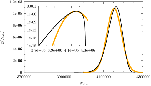
Figure 5: The exact distribution as computed by PATRONUS (black line) of the occurrences of the motif AAT in the human chromosome X for a Markov model of order $m=1$, considering an alphabet of five letters “ACGNT” to keep into account the gaps still present in current reference assembly. The obtained values for the statistical indicators are: $\operatorname{mean}=4153710$, $\operatorname{standard}\operatorname{deviation}=36587.1$, $\operatorname{skewness}=-0.635136$, $\operatorname{kurtosis}=18.5967$. As expected in this regime, the FMCI Gaussian approximation (orange line) is very good, providing a value of $4153790$ for the mean and of $36676.9$ for the average, and thus a substantially correct $z$-value; however, the distribution and its Gaussian approximation are actually very different, as clearly shown by the inset in logarithmic scale. In turn, if the gaps in the assembly are discarded and the standard alphabet is employed, the distribution looks almost perfectly Gaussian (not shown).

and Table 2), and of a set of more than 16.000 yeast transcription-factor binding sites (see Figures 6

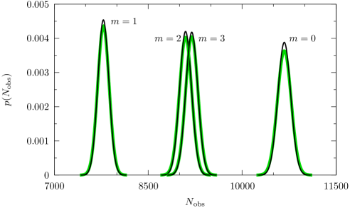
Figure 6: The exact distributions as computed by PATRONUS in S.cerevisiae for the TATA-box core sequence, TATAAA, considering all Markov models from order $0$ to $3$ (black lines). The FMCI Gaussian approximations are shown in green. Since $N_{\operatorname{obs}}=8635$, the pattern appears to be underrepresented in all the models apart from the case $m=1$.

and 7

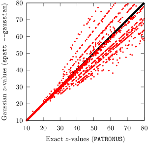
Figure 7: Graph of the $z$-values at $m=1$ of $\sim 3000$ transcription-factor binding sites in S.cerevisiae as computed by the Gaussian FMCI approximations vs. the exact results computed by PATRONUS. The transcription-factor binding sites have been extracted from 279 experimentally verified IUPAC templates. The graphs clearly show the regions where the approximation breaks down (that of large $z$-values). Note that for these examples PATRONUS is usually faster than the approximation (cf. Table 2).

). Neither problem can be practically approached with spatt (see Table 2, where timings on the smaller genomes of HIV and B.Subtilis are shown as well); furthermore, nothing would stop PATRONUS from examining the whole human genome ($\sim 3\cdot 10^{9}$ bases) in a feasible time. For example, assessing the relevance of all 320 3- and 4-letter patterns in the X chromosome at $m=2$ took only about 5 hours on our test machine.

A first general conclusion may be drawn from the many tests we performed: the method seems to work in a very fast and extremely reliable way for a broad interval of the parameter range. The only limitation is that the order $m$ of the Markov model employed should be $\leqslant 3$; in fact, for $m\geqslant 4$ the algorithm becomes unpractical, due to large computational times and, more crucially, to excessive memory requirements. This fact may be readily understood from Equations (6) and (9) which express the computational and memory costs, since by construction the number $s$ of states in the automaton is

$$s=a^{m}+\ell-1-m,$$

where $\ell$ is the length of the examined motif. On the other hand, in the range $0\leqslant m\leqslant 2$ the typical performance of the method is so good that it usually even consistently outperforms both the large-deviations and the Gaussian FMCI approximation of [3], as shown by Table 2. This is was matters practically, though, because using a Markov model with $m\geqslant 3$ typically implies severe uncertainty problems on the model itself [3].

The second main point is that our method always produces exact probability distribution functions from which all the information may be extracted; this can in principle allow for new interesting theoretical insights (see Figure 5).

Finally, our algorithm constitutes a very efficient benchmark for every possible approximate solution to the same problem (see Figure 7).

6 Conclusions

In this article, we show for the first time that a fast and accurate numerical evaluation of exact Markovian probability distribution functions in realistic cases of biological interest is possible. This is more and more important to get a reliable quantitative assessment of the relevance of biological sequences on the basis of their over- or under-representation, since the fast approximate methods used so far are known to systematically produce incorrect results. In fact, our algorithm retains the full ability of deducing all the relevant statistical information about motif occurrences, but its speed is comparable to that of some approximate algorithms, or even better in many cases: indeed, our successful analysis of motifs on the length scale of the human genome seems to prove that the exact Markovian approach should from now on be considered viable even on today’s computers. Thus, we hope that this result will open the way to a more widespread use of exact methods in the analysis of biological sequences.

References

- [1] L. Ettwiller, B. Paten, M. Ramialison, E. Birney, and J. Wittbrodt. Trawler: de novo regulatory motif discovery pipeline for chromatin immunoprecipitation. Nature Methods, 4(7), 2007.
- [2] G. Nuel. Effective -value computations using Finite Markov Chain Imbedding (FMCI): application to local score and to pattern statistics. Algorithms for Molecular Biology, 1, 2006.
- [3] G. Nuel. Numerical solutions for pattern statistics on Markov chains. Statistical Applications in Genetics and Molecular Biology, 5(26), 2006.
- [4] J. Zhang, B. Jiang, M. Li, J. Tromp, X. Zhang, and M. Q. Zhang. Computing exact -values for DNA motifs. Bioinformatics, 23(5):531 – 537, 2007.
- [5] P. Nicodème, T. Doerks, and M. Vingron. Proteome analysis based on motif statistics. Bioinformatics, 18:S161–S171, 2002.
- [6] M. A. Wright, P. Kharchenko, G. M. Church, and D. Segrè. Chromosomal periodicity of evolutionarily conserved gene pairs. PNAS, 104(25):10559 – 10564, 2007.
- [7] D. Halpern, H. Chiapello, S. Schbath, S. Robin, C. Hennequet-Antier, A. Gruss, and M. El Karoui. Identification of DNA motifs implicated in maintenance of bacterial core genomes by predictive modeling. PLoS Genetics, 3(9), 2007.
- [8] S. Robin, S. Schbath, and V. Vandewalle. Statistical tests to compare motif count exceptionalities. BMC Bioinformatics, 8(84), 2007.
- [9] S. Robin, F. Rodolphe, and S. Schbath. DNA, Words and Models: Statistics of Exceptional Words. Cambridge University Press, 2005.
- [10] A. Krogh, M. Brown, I. S. Mian, K. Sjölander, and D. Haussler. Hidden Markov models in computational biology: Application to protein modeling. Journal of Molecular Biology, 235:1501–1531, 1994.
- [11] A. V. Aho, M. S. Lam, R. Sethi, and J. D. Ullman. Compilers: Principles, Techniques, and Tools. Addison Wesley, 2 edition, 2006.
- [12] R. L. Graham, D. E. Knuth, and O. Patashnik. Concrete Mathematics. Addison-Wesley, Reading, Massachusetts, 1994.
- [13] G. Nuel. Pattern Markov chains: optimal Markov chain embedding through deterministic finite automata. Journal of Applied Probability, 2007.
- [14] W. H. Press, S. A. Teukolsky, W. T. Vetterling, and B. P. Flannery. Numerical Recipes in C. Cambridge University Press, 2002.
- [15] X. Leroy et al. http://www.ocaml.org, 2008.
- [16] M. Frigo and S. G. Johnson. The design and implementation of FFTW3. Proceedings of the IEEE, 93(2):216–231, 2005.
- [17] G. Nuel et al. http://stat.genopole.cnrs.fr/spatt, 2008.
- [18] P. Ribeca. http://www.paoloribeca.net/software/PATRONUS, 2008.